
1. Introduction
The subject of this paper originates from the Monte-Carlo simulations in Jiménez (Reference Jiménez2018b, Reference Jiménez2020a,Reference Jiménezb), whose purpose was to identify causally significant structures in two-dimensional decaying turbulence by inspecting the effect, after some predetermined time, of randomly perturbed initial conditions. These experiments will not be repeated here, and the reader is directed to the original publications for details. One of the most interesting results was that, besides the expected identification of individual vortices as significant (McWilliams Reference McWilliams1984, Reference McWilliams1990a), the experiments found that tight dipoles of counter-rotating vortices are as causally important as isolated vortices, or even more so. Modifying a strong vortex in the initial conditions leads to a large perturbation of the flow after five to ten eddy turnovers, but modifying a dipole leads to an even stronger perturbation. Co-rotating vortex pairs were not found to be significant in the same way.
The experiments mentioned above were intended to validate the Monte Carlo procedure, as well as to answer the fundamental question of whether some localised flow regions are more important than others for the evolution of the flow. They did not pay too much attention to the properties of the flow itself, being restricted, among other things, to a single relatively low Reynolds number. The present paper deals with the fluid mechanics. In particular, it examines whether our understanding of the evolution of two-dimensional turbulence can be improved by the consideration of collective structures, such as the dipoles mentioned above.
Several questions need to be addressed. The first one has to do with the Reynolds number, because one of the results in Jiménez (Reference Jiménez2020b) was that the preferred scale for significant vortices and dipoles is about the same, even if the vortices are associated with the enstrophy and the dipoles are structures of the kinetic energy. Spectral analysis shows that the typical scales associated with these two variables are different, but the Reynolds number in Jiménez (Reference Jiménez2020b) was not high enough to separate them clearly. To clarify this question, we analyse flow simulations at several Reynolds numbers, allowing, at least, for some range of scales.
The second question has to do with the role played in the flow by the two ‘templates’ (vortices and dipoles), and perhaps by other structures, because the original analysis was not concerned with the best representation of the flow, nor with flow mechanisms. Its only purpose was to identify which structures are most important from the point of view of dynamics, but not to clarify the dynamics itself. This problem is also connected with the Reynolds number, because flows at low Reynolds numbers essentially contain a single scale, which represents everything. More general flows are multiscale, and it is usually true that structures that represent well some aspect of the flow are not the ones that control the dynamics of others. For example, although vortices and vortex stretching (Vincent & Meneguzzi Reference Vincent and Meneguzzi1991) are considered good models for the turbulence energy cascade (Richardson Reference Richardson1920; Betchov Reference Betchov1956), at least from the point of view of enhancing dissipation, it was shown by Jiménez et al. (Reference Jiménez, Wray, Saffman and Rogallo1993) that removing them from the flow had very little lasting effect, and there is clear evidence of intermediate scales of the kinetic energy that are involved in the cascade process without being directly related to vorticity (Cardesa, Vela-Martín & Jiménez Reference Cardesa, Vela-Martín and Jiménez2017).
Much of the interest in two-dimensional turbulence originates from the remark by Onsager (Reference Onsager1949) that the inviscid evolution of a high-energy system of point vortices results in negative temperature states, and that this would naturally lead to the formation of organised coherent structures, rather than to a disordered flow.
There are at least two ways of approximating high-Reynolds-number two-dimensional turbulence by a conservative Hamiltonian system. The first one is the aforementioned system of point vortices (Batchelor Reference Batchelor1967), and the second is the approximation of the inviscid Euler equations in terms of Fourier components of the velocity, truncated to a finite range of wavenumber magnitude (Basdevant & Sadourny Reference Basdevant and Sadourny1975; Lesieur Reference Lesieur2008).
Kraichnan (Reference Kraichnan1967) followed the suggestion of Onsager (Reference Onsager1949) to propose that forced two-dimensional turbulence should include a reverse energy cascade towards larger scales, as well as a direct enstrophy cascade towards smaller ones. There is a fair agreement on the mechanism of the enstrophy cascade by means of vortex amalgamation and filamentation (McWilliams Reference McWilliams1990a; Carnevale et al. Reference Carnevale, McWilliams, Pomeau, Weiss and Young1991; Benzi et al. Reference Benzi, Colella, Briscolini and Santangelo1992; Dritschel et al. Reference Dritschel, Scott, Macaskill, Gottwald and Tran2008). The inverse cascade is less well understood, although it is generally believed that its mechanics is different from that of the enstrophy cascade and, in particular, that it is not predominantly mediated by vortex merging (Paret & Tabeling Reference Paret and Tabeling1998; Boffetta, Celani & Vergassola Reference Boffetta, Celani and Vergassola2000; Eyink Reference Eyink2006; Xiao et al. Reference Xiao, Wan, Chen and Eyink2009).
Kraichnan (Reference Kraichnan1967) derived the form of the spectrum of the truncated equilibrium Euler system, and observed that, in the absence of a low-wavenumber dissipation mechanism, energy would tend to accumulate at the largest system scale, in a process similar to the Bose–Einstein condensation of quantum systems. Both the reverse cascade and the condensate (Smith & Yakhot Reference Smith and Yakhot1993, Reference Smith and Yakhot1994) have been numerically and experimentally observed. A fair amount of work has gone into finding equilibrium solutions of the Euler equations that could account for this long-term flow behaviour, from vortex crystals (Aref et al. Reference Aref, Newton, Stremler, Tokieda and Vainchtein2002) to maximum entropy statistics (Joyce & Montgomery Reference Joyce and Montgomery1973; Montgomery & Joyce Reference Montgomery and Joyce1974), and there is numerical evidence that forced viscous two-dimensional flow locally relaxes to these inviscid equilibrium solutions (Montgomery et al. Reference Montgomery, Matthaeus, Stribling, Martinez and Oughton1992; Montgomery, Shan & Matthaeus Reference Montgomery, Shan and Matthaeus1993). For example, forced numerical turbulence in a square box evolves to a large-scale dipole filling the box diagonally (Smith & Yakhot Reference Smith and Yakhot1993). Recent reviews of the existing work on the reverse energy cascade and on condensate states can be found in Tabeling (Reference Tabeling2002) and Boffetta & Ecke (Reference Boffetta and Ecke2012).
Most of the work on the two-dimensional energy cascade has used forced experiments in which the system eventually settles to a statistically steady state. This has the advantage of allowing the use of ergodicity to compile statistics, but complicates the interpretation of the results because of the constant interference from the forcing. Decaying turbulence also has an inverse energy flux to large scales (although not necessarily an inverse cascade, as we will see later in the paper). The total energy remains approximately constant while its length scale grows until it collides with the domain size. From the point of view of causality characterisation, decaying turbulence has obvious advantages, because things happen only once, and the arrow of time is well defined. On the negative side, compiling reliable statistics requires ensembles of simulations, and the analysis of the resulting large data sets. The final stage of Bose condensation is also of little interest in this case, because the flow decays before it can be completed, but we will see in § 4 that a related process is important in the creation of large-scale structures.
In this paper, we study the dynamics of two-dimensional decaying turbulence, with emphasis on the mechanics of the inverse energy flux, using ensembles of simulations at low to moderate Reynolds numbers, guided by the results of the causality analysis mentioned at the beginning of this introduction. The simulations are described in § 2, followed in § 3 by the structural analysis of the flow in terms of the vortices, dipoles and streams suggested by the causal analysis. Section 4 describes the collective organisation of the vortices, including their classification into types and how each type is related to the large scales of the kinetic energy. Section 4.2 discusses mechanisms for this organisation, and § 5 concludes.
2. Simulations and basic flow properties
Simulations of decaying nominally isotropic two-dimensional turbulence are performed at various scale disparities in a doubly periodic square box of side  $L$, using a standard spectral Fourier code dealiased by the 2/3 rule. Time advance is third-order Runge–Kutta. The flow field is defined by its velocity
 ${\boldsymbol u}=(u,v)$ in the plane
 ${\boldsymbol x}=(x,y)$, and by the one-component vorticity
 $\omega =\boldsymbol {\nabla }\times {\boldsymbol u}$. It is initialised with random Fourier phases and a fixed isotropic enstrophy spectrum, which is relatively flat for small wavenumber magnitude
 $k$,
 $E_{\omega \omega }\sim k^{3/2}$, and much steeper,
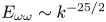 $E_{\omega \omega }\sim k^{-25/2}$, for large ones. The peak of this initial spectrum, located at
 $k_{init} \approx 2{\rm \pi} /L_{init}$, controls the initial energy-containing spectral range. The simulations solve the Navier–Stokes equations in vorticity–stream function formulation, using regular second-order viscosity,
 $\nu \nabla ^2\omega$.
Natural time and velocity scales can be defined from the root-mean-square (r.m.s.) vorticity magnitude  $\omega ' =\langle \omega ^2\rangle ^{1/2}$, where
 $\langle \cdot \rangle$ is the time-dependent ensemble average taken over the full computational box, and from
 $q' =(u'^2 + v'^2)^{1/2}$. The flow is allowed to evolve for
 $q' t_{init}/L=0.32$
 $(\omega 't_{init}\approx 6\mbox {--}12)$, after which the structures have established themselves. This moment is defined as the start of the simulations,
 $t=0$, for the rest of the paper, and is denoted by a ‘0’ subindex in the corresponding quantities. After some experimentation, the evolution of most quantities of interest for our argument was found to collapse best when plotted against
 $\omega '_0 t$, which will be used in the following. However, this collapse is not universal, and we could not find any normalisation for the time that would collapse well the evolution of all the flow properties, including some basic ones like the decay of the kinetic energy and of the enstrophy. As the simulation proceeds, the enstrophy decays by approximately 50 %, while the kinetic energy decreases at most by 5–10 %. A Taylor length scale can be defined as
 $\lambda _\tau =q'/\omega '$, and used to define a microscale Reynolds number,
 $Re_\lambda =q'\lambda _\tau /\nu$, where
 $\nu$ is the kinematic viscosity. Both grow by factors of 1.5–2.5 during each simulation, depending on the simulation time. Finally, each experiment is repeated at least 768 times to compile statistics, and a few cases were repeated twice as many times, to test convergence. These parameters are summarised in table 1.
Parameters of the simulations. The size of the doubly periodic computational box is  $L\times L$. The r.m.s. vorticity
 $\omega _0'$, and the velocity magnitude
 $q_0'$, are measured after the initial discarded transient, decaying from an initial enstrophy spectrum whose peak is at wavelength
 $L_{init}$. The Taylor microscale
 $\lambda _{\tau 0}= q_0'/\omega '_0$ is used to compute the Reynolds number
 $Re_\lambda =q'_0\lambda _{\tau 0}/\nu$, and
 $\lambda _{\omega 0}$ and
 $\lambda _{50}$ are the enstrophy and palinstrophy scales, respectively, defined in figure 1. The number of collocation points used before dealiasing is
 $N\times N$. The subscript ‘
 $F$’ refers to the end of each simulation, so that the decay time after the initial transient is
 $t_F$. Case T256 was used in Jiménez (Reference Jiménez2020b) to identify the causally significant structures used as starting points for the discussion in the text. Each case is an ensemble of 768 independent experiments.

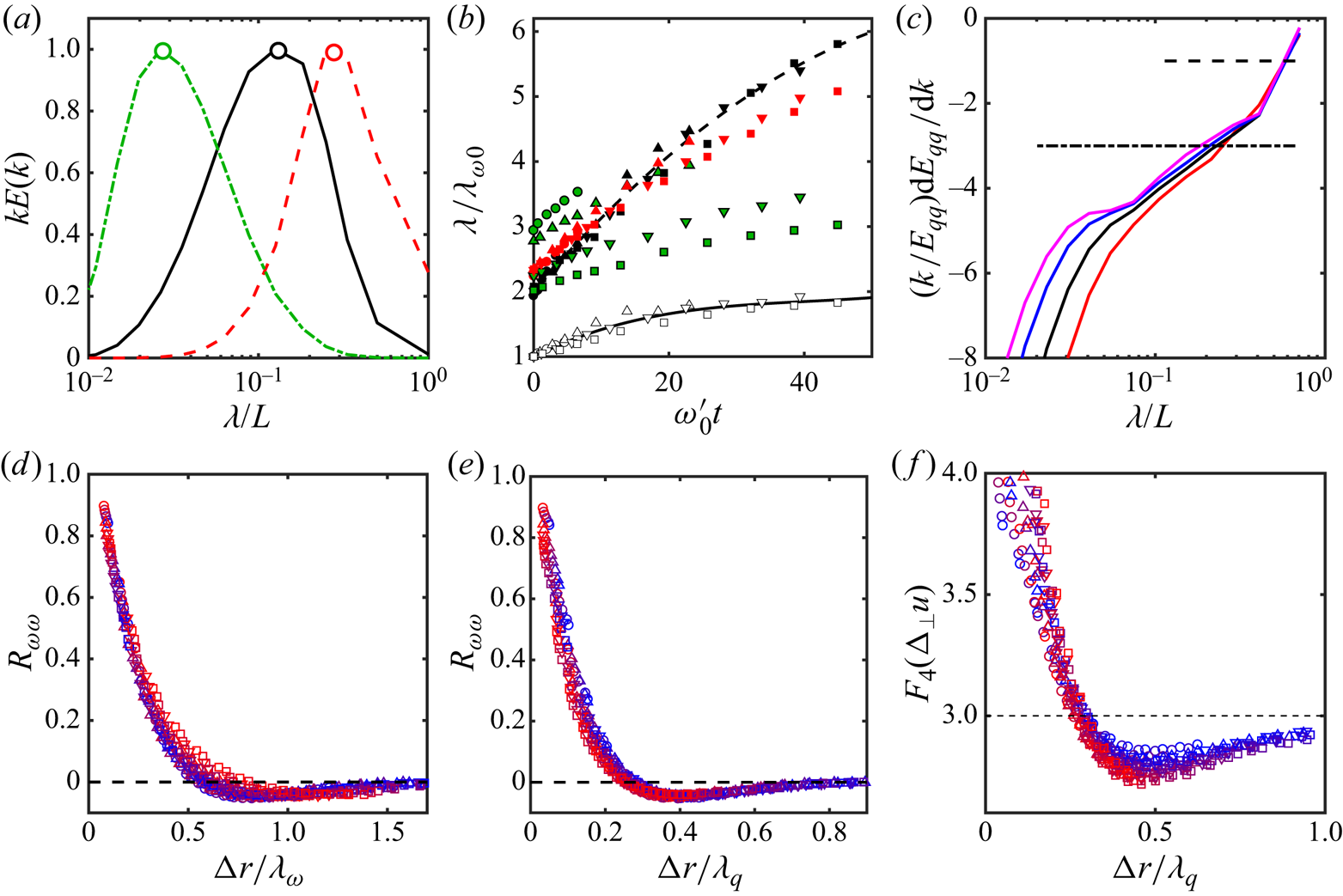
The evolution of the energy and enstrophy spectra is displayed in figure 1. For each simulation, time-dependent length scales for the vorticity and for the velocity can respectively be defined by the location of the maximum of the premultiplied enstrophy and energy spectra, as illustrated in figure 1(a). The enstrophy wavelength,  $\lambda _\omega =2{\rm \pi} /k_\omega$, increases only slowly with time, as shown in figure 1(b), but the energy scale,
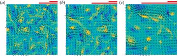
 $\lambda _q$, increases faster as the energy flows towards larger sizes. This is also clear from the snapshots in figure 2, which include scale bars for both wavelengths. Eventually,
 $\lambda _q\approx L$, at which moment the reverse energy flux saturates, and
 $\lambda _q$ stops growing (Smith & Yakhot Reference Smith and Yakhot1993). Although all our simulations were originally run for
 $\omega _0' t\approx 60$, only times for which
 $\lambda _q/L<0.6$ are included in figure 1(b) and in table 1. The flow is considered to enter afterwards into a different energy-condensation phase of its evolution, which is not discussed in this paper. Figure 1(c) displays the logarithmic slope of the energy spectrum. A plateau in this figure represents a power-law range, and the figure shows that no such range develops in our simulations at the level of
 $k^{-3}$, corresponding to the classical enstrophy cascade (Kraichnan Reference Kraichnan1967; Batchelor Reference Batchelor1969). Inspection of the temporal evolution of the spectrum (not shown) suggests that a weak inflection point may be developing at this level, but, since the spectra in figure 1(c) are plotted towards the end of each simulation, it is unlikely that a
 $k^{-3}$ range would ever develop in them. A slope
 $(k/E_{qq})\textrm {d} E_{qq}/\textrm {d} k=-3$ corresponds (algebraically) to the maximum of
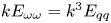 $k E_{\omega \omega }=k^3 E_{qq}$, which was used above to define
 $\lambda _\omega$. An extended
 $k^{-3}$ range would correspond to a flat top of the premultiplied enstrophy spectrum in figure 1(a). This does not happen, and the premultiplied enstrophy spectrum stays relatively sharp, as in figure 1(a). In the same way, a wavelength
 $\lambda _5$ can be defined by the maximum of the premultiplied spectrum of the vorticity gradient,
 $kE_{\boldsymbol {\nabla }\omega \boldsymbol {\nabla }\omega }= k^5 E_{qq}$ (figure 1a). The magnitude of this gradient is sometimes called the ‘palinstrophy,’ and controls the viscous dissipation of the enstrophy (Lesieur Reference Lesieur2008). We will therefore call
 $\lambda _5$ the palinstrophy wavelength. It is 3–5 times smaller than
 $\lambda _\omega$, and its initial value is given in table 1. It is the true viscous dissipative length for the flow, and the shortest of all the length scales defined here.
(a) Definition of the enstrophy, palinstrophy and energy peak wavelengths.  , Premultiplied enstrophy spectrum;
 , energy spectrum;
 , palinstrophy. Case T768 at
 $\omega _0' t =6.3$. (b) Evolution of the enstrophy and energy peak wavelengths; normalized with the enstrophy wavelength at
 $t=0$. Symbols as in table 1. Open symbols are enstrophy, and closed black ones are energy. The two polynomial fits are used as reference in later figures. The red closed symbols are the Taylor scale, stretched for clarity to
 $10\lambda _\tau /\lambda _{\omega 0}$, and the green ones are the stretched palinstropy wavelength,
 $10\lambda _5/\lambda _{\omega 0}$. (c) Logarithmic slope of the energy spectrum at the end of each simulation. From left to right, T1024 to T256. The two horizontal lines mark slopes
 $-1$ and
 $-3$, which respectively correspond to the energy and enstrophy peak wavelengths in (a). (d) Correlation function of the vorticity, as a function of the separation,
 ${\rm \Delta} r$, scaled with
 $\lambda _\omega$. Symbols as in table 1. Colours label time along each simulation for a fixed
 ${\rm \Delta} r$, from
 $t=0$ in blue to
 $t_F$ in red. (e) As in (d), scaled with
 $\lambda _q$. (f) Fourth-order flatness factor for the transverse velocity increments,
 ${\rm \Delta} _\perp u= u(x,y+{\rm \Delta} r)-u(x,y)$. Symbols and colours as in (d).

Vorticity and velocity field of a typical flow from T1024. From (a) to (c)  $\omega '_0 t=12.8$, 25.6, 64.2. The shorter bar on top of each figure is
 $\lambda _\omega$. The longer one is
 $\lambda _q$.

If we take  $\lambda _5$ to be a measure of the smallest vorticity structures, the numerical resolution of the simulations in table 1 is
 ${\rm \Delta} x/\lambda _5=0.1\text {--}0.2$, in terms of complex Fourier modes, and improves as the simulations proceed.
A logarithmic slope of  $-1$ coincides with the energy wavelength, and, because all the spectra in figure 1(c) are drawn just before the growth of
 $\lambda _q$ saturates in their respective simulations,
 $\lambda _q/L\approx 0.5$ in all cases.
It is interesting that the spectra in figure 1(c) develop a short but clear  $k^{-5}$ power law around the dissipative wavelength
 $\lambda _5$, especially for the higher Reynolds numbers. Spectra steeper than
 $k^{-3}$ are well known in two-dimensional turbulence, and are believed to originate from a variety of reasons that depend on the initial conditions. Saffman (Reference Saffman1971) argued that, since vorticity is conserved in the inviscid two-dimensional limit, the mutual distortion of the vortices eventually leads to the formation of vorticity discontinuities whose spectrum is
 $E_{\omega \omega }\sim k^{-2}$, or
 $E_{qq}\sim k^{-4}$. Brachet et al. (Reference Brachet, Meneguzzi, Politano and Sulem1988), starting from a relatively smooth vorticity field, report that a
 $k^{-4}$ energy spectrum appears initially, but evolves into
 $k^{-3}$ after individual vortices appear. This initial time (
 $\omega '_0 t\approx 10$) is of the same order as the transient period discarded in our simulations.
On the other hand, McWilliams (Reference McWilliams1984) and Benzi, Patarnello & Santangelo (Reference Benzi, Patarnello and Santangelo1987), whose initial conditions already include a  $k^{-3}$ spectral range, develop a steeper slope in the later part of the decay (
 $\omega '_0 t\gtrsim 100$ in our notation), when most of the vorticity is organised into individual cores that approximately behave as a conservative Hamiltonian system (Batchelor Reference Batchelor1967). They relate this steeper spectral slope to the vorticity distribution in the cores. This seems to be the case in our simulations, where the
 $k^{-5}$ plateau only develops towards the energy-condensed end of each simulation. We will mostly be interested in the earlier part of the evolution, where both the vortex cores and the ‘incoherent’ background vorticity are relevant. It should be noted that most of the simulations by the authors mentioned above use high-order hyperviscosity, which favours the formation of isolated vortices, instead of the regular viscosity in this paper.
Figures 1(d) and 1(e) display the autocorrelation function for the vorticity,
 \begin{equation} R_{\omega\omega}=\langle \omega(x,y)\omega(x+{\rm \Delta} r,y)\rangle/\omega'^2. \end{equation}
It has an inner core that scales with  $\lambda _\omega$ in figure 1(d), and an outer region that scales with
 $\lambda _q$ in figure 1(e). The scaling in figure 1(d) suggest that the diameter of the vortices that contribute to the correlation is
 $O(0.3\lambda _\omega )$. This will be confirmed when we study individual cores in § 3.2. At the moderate Reynolds numbers and regular viscosity of our simulations, the flow velocity is only slightly intermittent. The fourth-order flatness of the transversal velocity increments across a distance
 ${\rm \Delta} r$, is shown in figure 1(f). It also has two distance ranges. In an intermittent inner core of the order of the vortex diameter,
 ${\rm \Delta} r/\lambda _\omega \approx 0.3$, the flatness reaches
 $F_4\approx 4$. This part of the distribution does not collapse well in the figure, which is drawn to emphasise the return to Gaussianity at larger distances. The outer part of the distribution scales with
 $\lambda _q$. The flatness decays to the slightly sub-Gaussian value
 $F_4\approx 2.8$ at
 ${\rm \Delta} r/\lambda _q\approx 0.4$, and relaxes to the Gaussian
 $F_4\approx 3$ beyond
 ${\rm \Delta} r\approx \lambda _q$. The velocity itself is always close to Gaussian. Since the velocity gradient is known to be very intermittent near individual vortex cores, where it is dominated by the
 $1/r$ behaviour of the velocity (Jiménez Reference Jiménez1996), the return to Gaussianity marks the distance at which the flow is dominated by the interaction among several cores, instead of by individual ones. Figure 1(f) thus suggests that this typical distance among strong cores is
 $O(\lambda _q)$. This agrees with the outer scaling of figure 1(e), and will also be confirmed in § 3.2.
The Taylor microscale and the viscous length  $\lambda _5$ are included in figure 1(b), on a stretched vertical scale for clarity. Note that, although
 $\lambda _q$ and
 $\lambda _\tau$ collapse among the different simulations when normalised with
 $\lambda _{\omega 0}$, the viscous length
 $\lambda _5$ does not. The reason is uncertain, but relatively unimportant for the present paper, which is concerned with the large scales of the flow rather than with small-scale features. Viscous enstrophy dissipation is often described as being preceded by filamentation of the vortex cores under mutual stretching (Dritschel et al. Reference Dritschel, Scott, Macaskill, Gottwald and Tran2008), and
 $\lambda _5$ probably measures the width of these filaments and of the vortex fragments into which they decay.
It should also be noted that, although the Taylor scale is probably little more than an arbitrary length scale in three-dimensional turbulence, it has a deeper significance in two dimensions. We mentioned in the introduction the coexistence of two cascades in two-dimensional turbulence, and that they are connected in a general way with the form of the equilibrium spectrum of the truncated Fourier representation of the Euler equations. The only parameter in this spectrum is the ratio between the total kinetic energy and the enstrophy, which is the squared Taylor scale, and it can be shown that the limiting wavelength between the two cascades is proportional to  $\lambda _\tau$ (Basdevant & Sadourny Reference Basdevant and Sadourny1975; Lesieur Reference Lesieur2008). Whether an inverse cascade exists depends on whether this limit falls within the truncated set of Fourier wavenumbers, or, equivalently, on the ratio
 $\lambda _\tau /L$. It is difficult to make this criterion quantitative in viscous flows, whose spectrum is very far from equilibrium, but the growth of this ratio with time in figure 1(b) signals a shift of the kinetic energy towards larger scales.
3. Structural models
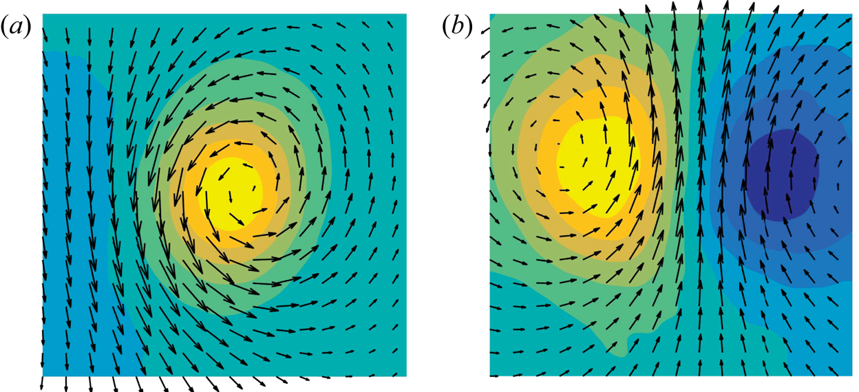
We saw in the introduction that the most interesting structural result in Jiménez (Reference Jiménez2020b) is that the causally significant flow neighbourhoods in two-dimensional turbulence look either like isolated vortices, or like counter-rotating vortex dipoles. The former was expected, because the classical model for this flow is a vortex ‘gas’ (McWilliams Reference McWilliams1984, Reference McWilliams1990a; Carnevale et al. Reference Carnevale, McWilliams, Pomeau, Weiss and Young1991; Benzi et al. Reference Benzi, Colella, Briscolini and Santangelo1992), but the latter was a mild surprise. The two models were summarised in Jiménez (Reference Jiménez2020b) by the archetypal ‘templates’ shown in figure 3. They were obtained by conditionally averaging the flow patches found to be most causally significant in the experiments described in the introduction. The patch size was found to be important, and, after some experimentation, it was adjusted to maximise the difference between significant and non-significant neighbourhoods. The optimum choice at the Reynolds number of Jiménez (Reference Jiménez2020b) are square patches of side  $L_p/L=0.1$, and the templates are constructed of side
 $L_T=3L_p$ to include some surrounding flow. But there is no reason to assume that this ‘most causal’ scale is also the one at which templates optimally represent the flow, or that the same dimensions work at different Reynolds numbers. Jiménez (Reference Jiménez2020b) showed that the first question could be answered by a posteriori optimisation of the approximation error between scaled templates and test flow fields. The application of this procedure to the present flows, and the answer to the second question, are tested below. Note that, when templates are used as archetypal flow structures, they lose their original connection with causal significance. They are treated as flow features that have been found to be of interest ‘for some reason,’ and the issue becomes to find what they are, and whether they can be used as indicators of some aspect of the flow dynamics. Why they were causally significant in the first place can be addressed a posteriori, if desired. For more details on the process of template extraction, verification and validation, the reader is directed to Jiménez (Reference Jiménez2018b) and Jiménez (Reference Jiménez2020b).
Vorticity and velocity field for the templates identified in Jiménez (Reference Jiménez2020b) as the most causally relevant flow features. (a) Vortex template, mostly relevant for experiments manipulating vorticity. (b) Dipole template, relevant for velocity manipulations. Because the position, scale and intensity of the templates are adjusted when matching the flow, their orientation, size and intensity are arbitrary.

To test how well a template approximates a particular flow neighbourhood, it is first scaled to size  $L_T\times L_T$, optimally oriented (using four orthogonal rotations and one reflection), and its intensity is adjusted to match the overall r.m.s. intensity of the flow in question, so that
 $\langle \xi _T^2\rangle _T =\xi '^2$. The ‘
 $T$’ subindex here represents template properties, as well as averaging over the template domain, and
 $\xi$ is either the vector velocity or the scalar vorticity. Centring the rescaled template at some point,
 ${\boldsymbol x}$, the representation error is measured as the relative
 $L_2$ norm of the difference between the flow and the template,
 \begin{equation} \varPhi_\xi ({\boldsymbol x},L_T) = \frac{\|\xi({\boldsymbol x}+\tilde{{\boldsymbol x}})-\xi_T(\tilde{{\boldsymbol x}})\|_{\tilde{{\boldsymbol x}}\in T}}{\|\xi\|_T}, \end{equation}
which is a function of  $L_T$ and of
 ${\boldsymbol x}$. Statistics are compiled over all the positions in an
 $N_t\times N_t$ ‘test’ grid, and over all the flow realisations, and scanned over
 $L_T$.
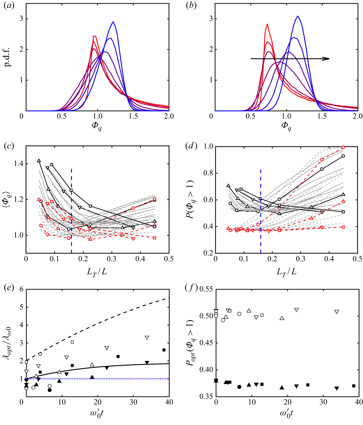
Typical probability density functions (p.d.f.s) of the approximation error are given in figure 4(a,b) as functions of the template size. The peak of the histogram generally moves to smaller errors as  $L_T$ decreases, and becomes very skewed, especially for dipoles, suggesting the necessity of using several figures of merit to quantify the overall performance of a template. An obvious choice is to minimise the mean error,
 $\langle \varPhi _\xi \rangle (L_T)$, where the average is taken over all the template positions. It provides an overall goodness of fit, but the shape of the histograms in figure 4(a,b) suggests that it may mix some very good local fits with some very bad ones. Coherent structures can be relevant to the flow dynamics even when they fill a relatively small area fraction (Jiménez Reference Jiménez2018a), and a representation of the flow in terms of them should be able to stress the good fits even at the expense of de-emphasizing some of the bad ones. A measure with this property is the fraction of the p.d.f. above a given error threshold. We use
 $P_{\xi }=\mbox {prob.}(\varPhi _\xi >1)$. The behaviour of both measures with template size is shown in figure 4(c,d), and depends on the particular case and on the simulation time considered. Most cases are displayed as light grey lines, without identification, to show general trends, but the final time of each simulation, defined by
 $\lambda _q/L\approx 0.6$, is highlighted and labelled with the symbols in table 1.
(a,b) Probability density function of the template approximation error. Energy error norm. Case T512,  $\omega '_0 t=9.2$. Template size, increasing from red to blue:
 $L_T/L=0.045$, 0.08, 0.11, 0.22, 0.34, 0.45, 0.56. (a) Template is a vortex. (b) Template is a dipole. The arrow is in the direction of increasing template size,
 $L_T$. (c,d) Approximation error as a function of case and of
 $L_T$. Cases are plotted for different times as grey lines without labels, except for the final time of each simulation, which is highlighted and labelled as in table 1.
 , Template is a vortex;
 , template is a dipole. The dashed vertical line is a representative value of
 $\lambda _\omega /L$, from table 1. (c) Error is averaged over all template positions. (d) Error measured as the fraction,
 $P_q$, of relative local errors larger than unity. (e) Template size for optimum
 $P_q$. Lines are the polynomial fits to
 $\lambda _\omega$ and
 $\lambda _q$ in figure 1(b). Closed symbols are dipole templates; open symbols are vortex templates. (f) As in (e), showing the optimum
 $P_q$.

At short simulation times (grey lines), figure 4(c) shows that the average error,  $\langle \varPhi _q \rangle$, is minimum for template sizes of the order of
 $\lambda _\omega$, but that the optimum size increases with time and with the Reynolds number. The optimum template size for some of the longest simulations is the largest one allowed by the computational box,
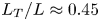 $L_T/L\approx 0.45$. Larger templates are considered in this paper to be contaminated by the box size, and are not included in the analysis. This behaviour holds for vortices (solid lines), and for dipoles (dashed lines).
Figures 4(d) and 4(e) show that the fraction,  $P_{q}$, of large kinetic-energy error tends to be minimised by small templates of the order of the diameter of the intense vortices seen in figure 2. This fits the intent of this measure, which is to identify local structures. It is interesting that this preference for small features is clearest for the dipole template, while the optimum size for the vortex template tends to be larger. Both optimum sizes increase with the evolution time and with the Reynolds number. Figure 4 uses the kinetic-energy norm. The results for the enstrophy norm are similar, with a preference for slightly larger templates.
Figure 4(f) shows that the approximation error attained at the respective optimum size changes little among simulations and among simulation times, even if we have seen that the optimum size varies widely. The optimum mean error is approximately  $\langle \varPhi _q\rangle =1.04,\ \langle \varPhi _\omega \rangle =1.22$ for vortices and
 $\langle \varPhi _q\rangle = 0.98,\ \langle \varPhi _\omega \rangle =1.12$ for dipoles. The minimum error fraction is
 $P_{q}=0.51,\ P_{\omega }=0.81$ for vortices and
 $P_{q}=0.37,\ P_{\omega }=0.62$ for dipoles. Interestingly, dipoles are always more successful templates than isolated vortices, and the kinetic-energy error is always lower than the enstrophy one. We will almost exclusively discuss dipole templates and the kinetic-energy norm for the rest of this section.
3.1. Large-scale streams
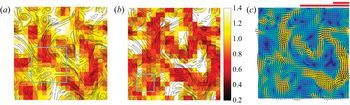
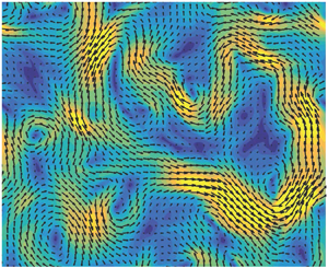
Figures 5(a) and 5(b) are heat maps for the fit of the vortex and dipole templates to a typical flow snapshot. The intensity in a heat map is proportional to the goodness of fit of the template centred at that point. The darker regions in figure 5 represent better fits, measured by  $\varPhi _q$. Figure 5(a) is drawn for vortex templates, and figure 5(b) is drawn for dipoles. In both cases, the size of the template is chosen to be optimum, which in this particular case is different for the two templates (see the cyan boxes in the figure). Inspection of the figures shows that the features extracted by the two templates have much in common, although they differ in detail. This is not surprising because a dipole is formed by two vortices, and it was to be expected that at least some of the vortices identified by a vortex template are part of a dipole.
(a,b) Heat maps for the fit error of a typical flow field. Case T768 at  $\omega '_0 t=22$. Colour represents the approximation error,
 $\varPhi _q$, for a template centred at each point. Line contours are the vorticity magnitude. The cyan box is the size of the template, chosen in each case to optimise
 $P_q$. (a) Vortex template. (b) Dipole template. (c) Velocity field for the flow in (a,b). The scale bars above the figure are as in figure 2. The background colour is the velocity magnitude, lighter for faster velocities.

However, the main use of heat maps is not to identify individual features, but to highlight the organisation of the features themselves. Thus, although we have mentioned that figures 5(a) and 5(b) differ in detail, it is visually clear that they cluster around a common large-scale structure, present in both figures. Its nature is clearer in figure 5(c) which shows that it is a meandering stream that spans the full box. This is interesting for two reasons. The first one is that it suggests that the feature detected by the dipole template is not the pair of vortices, but the jet between them. The second one is that those jet segments are part of a larger stream, too large and too irregular to be represented by any local template, but which can be recovered by the concatenation of several of them.
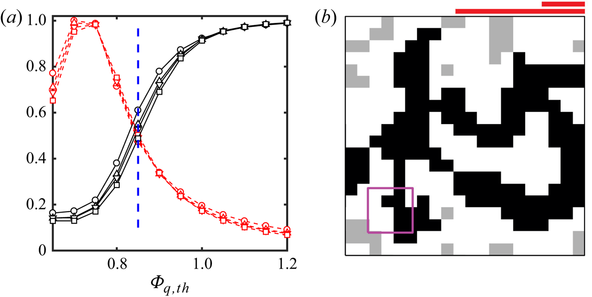
Figure 6 shows how this large-scale flow organisation can be defined by thresholding the heat map below a given error level. The resulting points are collected into individual objects, defined by contiguity along the four directions of the coordinate axes. Figure 6(a) is the percolation diagram (Moisy & Jiménez Reference Moisy and Jiménez2004). The solid lines represent the fraction of the total thresholded area contained in the largest contiguous thresholded object. It is unity for very high thresholds, where a single object fills the whole field, and also for a lowest limit in which a single point represents both the whole thresholded region and its largest object. Neither limit gives information about the structure of the flow, and both are left outside figure 6(a), which centres on the intermediate range in which several individual low-error objects first appear and then merge into larger ones as the threshold is raised. The dashed lines are the number of individual objects, normalised to unit maximum. The percolation diagram is averaged over all the times of each simulation, and varies little among simulations. After some experimentation, the reference threshold is chosen to be  $\varPhi _{q,th}=0.85$, which is used in figure 6(b) to threshold the map in figure 5(b). There is a dark largest connected object, and several smaller ones in a lighter colour, which are also below the error threshold but which are not connected to the largest one. They will not be used when compiling the statistics of the large flow scales. The percolation transition is narrow, and changing the threshold by any large amount moves the result into either an empty or a completely full map, but thresholds in the range 0.8–0.9 yield approximately the same results as those presented below.
Definition of the largest thresholded structure in each snapshot. (a) Percolation diagram for  $\varPhi _q\le \varPhi _{q,th}$, as a function of the threshold. Dipole templates optimised for
 $P_{q}$. Solid lines are the area of the largest thresholded object divided by the total thresholded area. Dashed lines are the number of objects, normalised to unit maximum. Individual lines are for each simulation, with symbols as in table 1. The vertical dashed line is the standard threshold used below. (b) Thresholded heat map from figure 5(b). The darker object is the largest connected structure, used in the following to represent the large-scale flow organisation, and the purple box is the template size.

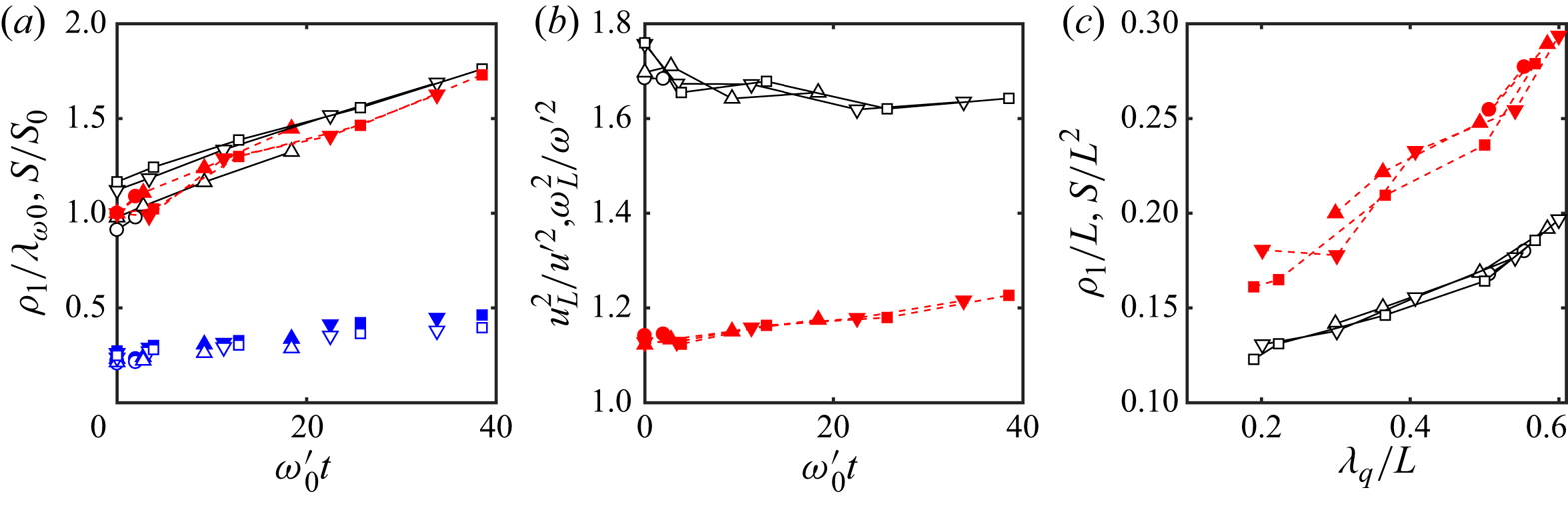
It should be understood that heat maps and their thresholded versions are at most ‘skeletons’ of flow properties. Each point of the map is an element of the  $N_t\times N_t$ ‘test’ grid used to test the template approximation properties. It marks the centre of a template box, but the optimum template size is generally wider than the spacing of the test grid, as shown in figures 5 and 6. Any geometric property of the skeletons should be interpreted with this in mind. For example, the solid lines in figure 7(a) show the inner ‘width,’
 $\rho _1$, of the largest thresholded object in each frame, defined as the side of the largest square that completely fits within the object (Catrakis & Dimotakis Reference Catrakis and Dimotakis1996; Moisy & Jiménez Reference Moisy and Jiménez2004). The figure is compiled over a test grid with
 $N_t=20$, so that the minimum possible value is
 $\rho _1/L=0.05$. This is smaller than the widths in figure 7(a), which are of the order of
 $\lambda _{\omega 0}\approx 0.15$ (table 1), but close enough to it to recommend testing whether
 $\rho _1$ is influenced by the test grid. Limited testing with
 $N_t=30$ shows that the results in figure 7(a,b) could change by approximately 15–20 % on a much finer test grid.
Properties of the largest thresholded structure of low  $P_q$ in each snapshot. (a) Temporal evolution of the geometry of the largest structure.
 , Inner scale normalised with the initial enstrophy scale,
 $\rho _1/\lambda _{\omega 0}$;
 , area of the largest structure normalised with its initial value,
 $S/S_0$; symbols without lines are the integral length
 $L_{int}/\lambda _{\omega 0}$ for the correlations of
 $\varPhi _q$, defined in (3.2). Symbols as in table 1. Open symbols are vortex templates; closed symbols are dipoles. (b) Flow properties within the largest structures.
 , Kinetic-energy density;
 , enstrophy density. (c) As in (a), but unnormalised, versus the kinetic-energy wavelength.

The symbols without lines in figure 7(a) are the integral length,
 \begin{equation} L_{int}= \int_0^\infty C_{\varPhi\varPhi}(r) \,\textrm{d} r,\end{equation}
derived from the radial autocorrelation function of the approximation error,  $\varPhi _q$, which typically measures the narrowest dimension of the structures of that variable. It is interesting that, even if we have seen that the approximation error is a marker for the largest, energy-containing scales in the flow, the integral length is narrower than the enstrophy peak in figure 1. In fact, its typical value,
 $0.3\lambda _{\omega 0}\approx 0.05 L$, is of the order of the spacing,
 $L/N_t$, of the test grid over which it is computed, and could actually be shorter in a finer grid. If we take
 $L_{int}$ to represent the average thickness of the structures of
 $\varPhi _q$, it would imply that the snapshot in figure 6(b), where the thickness of the structures is of the order of the test cell, is indeed typical.
Note that, since the length of the structures can be estimated by  $S/\rho _1$, the fact that
 $S$ and
 $\rho _1$ grow at a similar rate in figure 7(a) implies that the length of the structures changes little as the flow evolves
 $(S/\rho _1L=1.3\to 1.5)$, but that their aspect ratio grows ‘fatter’
 $(S/\rho _1^2=11\to 8)$. We will see below that the longitudinal scale of the structures is typically of the order of the box size, and, therefore, presumably limited by it.
Figure 7(b) shows kinetic energy and enstrophy averaged over dipole templates centred on points within the largest thresholded object in each snapshot. As suggested by figure 5(c), and by the definition of the dipole template in figure 3(b), dipoles contain locally high kinetic energy, but also moderately high enstrophy. Interestingly, enstrophy is less concentrated than the energy. It could be expected that, since the edge of a jet is necessarily the seat of high vorticity, the ‘fringe’ of grid points surrounding the large-scale thresholded streams would be regions of especially high enstrophy, but this is not true. When energy and enstrophy are conditioned to that fringe, the kinetic-energy density is lower than the average, and the enstrophy density is indistinguishable from the mean (not shown). A similar result holds for other flow regions outside the streams. The only high-energy regions are apparently those detected by the dipole template, including the lighter-grey regions in figure 6(b), and the only moderately high enstrophy regions are also, on average, associated with the streams.
Perhaps the strongest indication of the connection of the streams with the structure of the kinetic energy is figure 7(c). The quantities in figure 7(a) are normalised with their initial value because they do not otherwise collapse. The initial conditions, which are chosen to provide a variety of scale combinations, are too different to allow it. For example, the average value of the area of the largest stream at  $t=0$ varies by 60 % among the different simulations. On the other hand, figure 7(c) shows the unnormalised area and thickness of the large streams versus the energy wavelength,
 $\lambda _q$. They collapse well, strongly suggesting that the streams are the support of the kinetic energy of the flow, and that the process of stream formation is tantamount to the flux of the energy to larger scales.
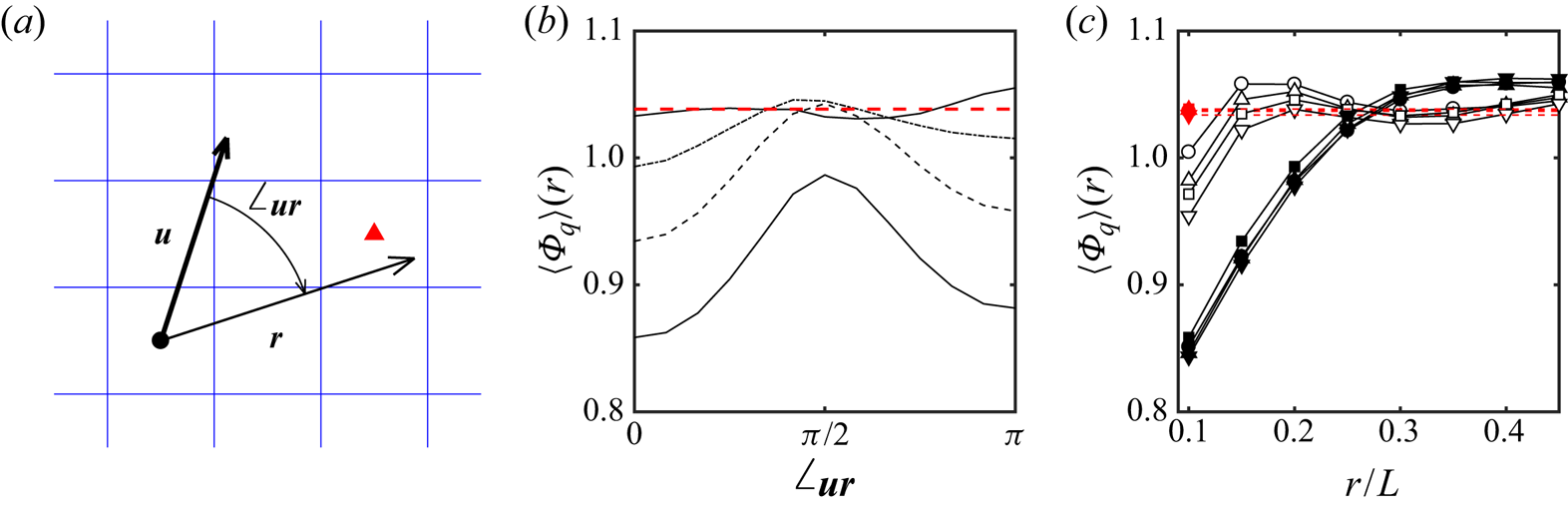
Figure 8 tests whether the structures detected by the concatenation of dipoles are elongated and aligned with the flow velocity, as suggested by figure 5(c). Consider the sketch in figure 8(a). For a given flow snapshot and template size, each cell in the  $N_t\times N_t$ test grid has an associated flow velocity,
 ${\boldsymbol u}$, and an approximation error,
 $\varPhi$, defined by averaging over the domain of the optimal template centred on it. Choosing a displacement vector
 ${\boldsymbol r}$ with respect to this point, figure 8(b,c) shows the average of the approximation error corresponding to the cell whose centre is closest to the end of
 ${\boldsymbol r}$. The figure shows the mean error conditioned to the magnitude of
 ${\boldsymbol r}$ and to its angle,
 $\angle _{\boldsymbol{\textit{ur}}}$, with respect to
 ${\boldsymbol u}$. When this conditional mean is averaged over all the points of the test grid, the result is essentially independent of the angle, and similar to the unconditional mean of the error. But, when the conditional centre is chosen within the largest low-error structure in each flow field, figure 8(b) shows that points aligned with the velocity,
 $\angle _{\boldsymbol{\textit{ur}}}=0$ or
 $\angle _{\boldsymbol{\textit{ur}}}={\rm \pi}$, preferentially contain low approximation errors, while those perpendicular to it have high ones. This effect weakens with the length of
 $r$, but figure 8(c) shows that it persists for a distance of the order of
 $0.25 L$, which is four or five times longer than the width
 $\rho _1$ in figure 7(a). It is interesting that the distance at which the minimum error in figure 8(c) reverts to its unconditional value is approximately the same for the four cases included in the figure. In fact, it changes little among all the cases tested, showing that the longitudinal scale of the high-velocity streams is always of the order of the box size. The growth of the energy wavelength,
 $\lambda _q$, in figure 1(b) and of the area of the high-energy region in figure 7(a) is presumably due to more convoluted streams, rather than to longer-range ones.
Mean approximation error conditioned to the orientation with respect to the velocity. (a) Definition sketch. (b) Mean error as a function of the orientation angle. T1024 at  $\omega '_0 t=39$. From bottom to top, distance to the reference point:
 $r/L=0.1\ (0.05)\ 0.25$. (c) Streamwise and transverse conditional errors as functions of the distance to the reference point. Symbols as in table 1, with each case at its final simulation time. Closed symbols are measured aligned with the velocity, and open ones are measured at right angles to it. The dashed horizontal lines in (b,c) are unconditional errors.

An intriguing feature of figure 8(b) is the asymmetry between the conditional error at  $\angle _{\boldsymbol{\textit{ur}}}=0$ and
 $\angle _{\boldsymbol{\textit{ur}}}={\rm \pi}$. Since each point in the low-error structures is both the origin and the end of some conditioning vector, both directions could be expected to be equivalent. But they are not, and the error is lower in front of the conditioning point than behind it. The effect is small but statistically significant; the estimated standard deviation of the lines in figure 8(b) is only slightly larger than the width of the lines. It is also consistently found in all the cases examined, not only in the one chosen for the figure. This result is difficult to interpret, but the implication is that the direction of the velocity is a better predictor of the downstream location of the low-error structures than of their upstream location. We will come back to this point in § 4.2.
3.2. Vortices
Even if this paper is mostly concerned with the large energy-containing structures of the flow, there is no doubt that two-dimensional turbulence can also be described as a collection of coherent vortices (McWilliams Reference McWilliams1984, Reference McWilliams1990a; Benzi et al. Reference Benzi, Colella, Briscolini and Santangelo1992). The question that interests us here is whether the large-scale structure discussed above for the kinetic energy can be described in terms of the organisation of these vortices. In this section we first address the properties and evolution of the vortices themselves.
Figure 9(a) shows a segmentation of a typical flow field into individual vortices, defined as connected regions in which  $|\omega |\ge H\omega '$. As in the case of figure 7, the vorticity of the flow separates into a few large connected objects for
 $H\ll 1$, and breaks into more numerous smaller objects as
 $H$ increases. Beyond a certain threshold, the number of vortices decreases again, and eventually vanishes when no vorticity satisfies the thresholding condition. The value
 $H=0.9$ used in figure 9 is chosen to maximise the number of individual vortices (Moisy & Jiménez Reference Moisy and Jiménez2004). To gain some sense of the importance of vortex interactions, the vortices in figure 9(a) are grouped into co- and counter-rotating pairs. Two vortices are considered a potential pair if their area,
 $s$, differs by less than a factor of
 $m^2$, which is an adjustable parameter. The underlying rationale for this restriction is that very dissimilar vortices are unlikely to form long-lived pairs, because the larger one would tear the smaller one apart (Meunier, Le Dizès & Leweke Reference Meunier, Le Dizès and Leweke2005). The figure uses
 $m=2$, but statistics compiled with
 $m=1.5$ and
 $m=3$ show no substantial differences (see Jiménez Reference Jiménez2020b). Vortices are paired to the closest unpaired neighbour within their area class, and no vortex can have more than one partner. Some vortices find no suitable partner, and are left unpaired.
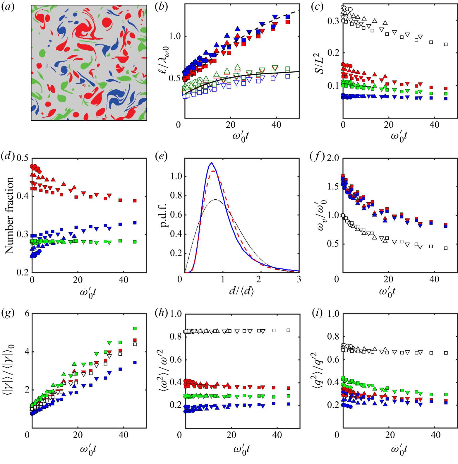
Properties of the thresholded vorticity structures. (a) Typical segmented image. Case T1024,  $\omega '_0t=39$. In all the panels in this figure, unless otherwise noted, red are dipoles, blue are co-rotating pairs and green are isolated vortices. Other symbols as in table 1. (b) The open symbols are the mean diameter of the vortices, and the closed coloured ones are the distance between vortices in a pair. Lengths are normalised with the vorticity wavelength at
 $t=0$, and the trend lines are the polynomial fits from figure 1(b) to:
 ,
 $0.3\lambda _\omega$;
 ,
 $0.22 \lambda _q$. (c) Area fraction covered by all the vortices of a given class. Open symbols include all the classes. (d) Number fraction of vortices in different associations. (e) Probability density function of the distances between vortices in a pair. Colours as in (a), but the chain-dotted black line is the distribution for a Poisson point set. (f) Mean vorticity of the vortex cores. Symbols in (f–i) are as in (c). (g) Average circulation of the vortex cores. (h) Enstrophy fraction contained in the different vortex associations. (i) As in (h), for the kinetic energy.

Figure 9(b) displays mean values of the diameter,  $s^{1/2}$, and of the distance
 $d$ between the centres of gravity of the component vortices of the pairs, compiled at several evolution times for each set of simulations. The diameter of the vortices depends very little on how they are paired, and, in agreement with the estimations from the vorticity and velocity statistics in figure 1, is described well by a fraction of the vorticity wavelength,
 $0.3 \lambda _\omega$. The distance between the vortices of a pair is initially somewhat larger, of the order of
 $0.5 \lambda _\omega$, but it grows with
 $\lambda _q$, faster than
 $\lambda _\omega$. The approximate similarity between the inter-vortex distance and their diameter implies that vortex pairs remain tightly packed at this stage of their evolution, although the faster growth of the average distance means that the area fraction covered by the vortices slowly decays (figure 9c). It should be noted at this point that the absolute value of the intra-pair distance in figure 9(b) offers a possible explanation of the observation in § 3.1 that the edges of the high-speed streams are not a concentration of high enstrophy. It follows from comparing figures 7(a) and 9(b) that
 $d$ is 2–3 times narrower than the width
 $\rho _1$ of the jets, so that, if these jets are defined as in figure 7, the dipoles are contained within them, rather than at their border. This is consistent with the visual inspection of the snapshot in figure 5(b).
Figure 9(d) shows the number of vortices involved in different kinds of pairings, giving a rough measure of the importance of the different interactions. Most vortices are in the form of pairs. Of the approximately  $2\times 10^6$ vortices represented in figure 9, 43 % form dipoles, 29 % are in co-rotating pairs and 28 % are isolated, with a tendency of the number of dipoles and co-rotating pairs to converge as the Reynolds number increases. Similar values were found by Jiménez (Reference Jiménez2020b) at the lowest of the four Reynolds numbers used in the present paper. The difference between the number of co-rotating and counter-rotating pairs is also encountered in the covering fraction in figure 9(c), and is a property of the flow that disappears if the vortex position is randomised. On the other hand, the scarcity of unpaired vortices is a geometric property that persists when the pairing algorithm is applied to a set of Poisson-distributed points.
In fact, a random distribution of the vortex position is a reasonable lowest-order model for their local organisation. Even if the vortex diameter and the intra-pair distance grow by a factor of approximately two during the simulation time, the form of their p.d.f. stays remarkably constant. For example, figure 9(e) shows the p.d.f. of the distance among the components of vortex pairs, normalised by their mean for each individual experiment. The figure also includes the p.d.f of a set of Poisson-distributed points with the same mean. The distribution of dipoles and co-rotating pairs are very similar, with a weak tendency of dipoles to be farther apart. The Poisson distribution is wider, but most of the discrepancy can be explained by the exclusion of pairs whose separation is smaller than the vortex diameter (see appendix A). This explanation is confirmed by the distribution of the distance  $d$ between all possible couples of vortices (not shown). This distribution should be proportional to
 $d$ for any homogeneous flow, but this is only true for
 $d \gtrsim 2\langle s^{1/2}\rangle$. Shorter distances are essentially missing.
In the same way, there is relatively little difference between the properties of vortices in dipoles and those in co-rotating pairs. We saw in figure 9(b) that their diameters are similar, and figure 9(f) shows that so are their vorticities, which decay at the same rate as the r.m.s. vorticity of the flow. On the other hand, some explanation is needed for figure 9(c,d), which shows that both the number of dipoles and the total area covered by them is larger than those of co-rotating pairs. A similar difference appears in figure 9(g), which shows that the average vortex circulation magnitude grows linearly for all classes. The circulation of a vortex core can only grow by merging with other cores or by entraining background vorticity, since there is no vorticity source in two dimensions, but the average over a class is also influenced by the transfer among classes. Figure 9(g) shows that the circulation of dipoles is typical of the overall average (they are the largest contributors to it), but that co-rotating pairs grow more slowly, while unpaired vortices grow slightly faster than the average. The simplest explanation is that co-rotating pairs tend to merge into single (initially unpaired) cores (Meunier et al. Reference Meunier, Le Dizès and Leweke2005), thus depleting their number, while dipoles are longer lasting (Flierl et al. Reference Flierl, Larichev, McWilliams and Reznik1980; McWilliams Reference McWilliams1980).
Figure 9(h) shows the fraction of overall enstrophy contained in the thresholded vortices. Over 85 % of the total enstrophy is contained in them, and this fraction is remarkably constant among Reynolds numbers and time, no doubt, in part, because the vorticity threshold used to identify them is a constant fraction of the r.m.s. vorticity. The contribution to the enstrophy of the different vortex classes is in line with the area fraction in figure 9(c), as could be expected from the similarity of vortex properties discussed above.
The fraction of the kinetic energy due to the vortices is harder to define. The simplest definition is the fraction of  $q'^2$ retained by a flow reconstructed from the vorticity contained within a given class of thresholded vortices. Figure 9(i) shows that keeping all the thresholded vortices retains 65–70 % of
 $q'^2$, while keeping only the dipoles or the co-rotating pairs retains 25–30 % of the energy, and keeping only the unpaired vortices retains 30–40 %. The change in the relative contribution of dipoles to the enstrophy in figure 9(h) and to the energy in figure 9(i) is interesting. While dipoles predominate in number, area and enstrophy, their contribution to the energy is of the same order as the co-rotating pairs, and substantially less than the unpaired vortices. In fact, even if dipoles contain a local jet of high velocity, their overall kinetic energy is lower than for co-rotating pairs, because the total circulation of a dipole is zero, and its induced velocity falls with distance much faster than for a co-rotating pair (Batchelor Reference Batchelor1967). Even if decaying turbulence is very far from an equilibrium system, Benzi et al. (Reference Benzi, Colella, Briscolini and Santangelo1992) and Dritschel et al. (Reference Dritschel, Scott, Macaskill, Gottwald and Tran2008) have shown that an approximately Hamiltonian system of point vortices, punctuated by the occasional merger of like-signed vortices, is a good approximation to the late stages of two-dimensional enstrophy decay. The difference in the interaction energy of dipoles and co-rotating pairs is probably also part of the reason for their different behaviour, and for the slower decay of the former through amalgamation.
In summary, the vortex evolution discussed in this section is consistent with the description of decaying two-dimensional turbulence as a system of discrete vorticity structures (McWilliams Reference McWilliams1984; Benzi et al. Reference Benzi, Patarnello and Santangelo1987; Brachet et al. Reference Brachet, Meneguzzi, Politano and Sulem1988), although, at the relatively early stage of the decay studied here, the structures cannot be described as either equilibrium or isolated. Their self-similar growth through amalgamation accounts for the gradual increase in the vorticity scale,  $\lambda _\omega$, but the sizes involved are always much smaller than the energy scale,
 $\lambda _q$ (see the scale bars in figure 2).
It is interesting that the Reynolds number of the individual vortex cores stays relatively low during the simulations,  $Re_\gamma =\langle \gamma \rangle /4{\rm \pi} \nu \approx 1.5 \to 7$. Since the maximum vorticity of a viscously decaying circular vortex satisfies
 $\omega t =Re_\gamma$ (Batchelor Reference Batchelor1967), where the left-hand side is time measured in turnovers, it follows that the size of the vortices in the simulations, even as they grow by accretion, is typically controlled by viscosity.
4. Collective structures
4.1. Vortex organisation
In fact, the question of how vortices organise themselves to create the streams discussed in § 3.1 remains open. One possibility, already mentioned, is that the streams are concatenations of dipoles that are responsible for short segments of the stream. We saw in the discussion of figure 9 that this model is compatible with the observed vortex distances and dimensions, but the open question is how the individual dipoles align themselves into longer units. Another model is that the streams are contact interfaces between large-scale vortices. We saw in figure 9(b) that the mean vortex diameter increases only weakly during even the longest flow evolution, and that it is always much smaller than the kinetic-energy wavelength, but it is possible that the small cores organise themselves into large-scale vortex ‘bags’ that fill the space between the streams, acting as coherent structures from the point of view of the kinetic energy (Paret & Tabeling Reference Paret and Tabeling1998; Tabeling Reference Tabeling2002). However, we saw in § 3.1 that the only concentration of vorticity is within the coherent jets, not between them.
The crucial uncertainty is the intensity of the interaction among vortex cores, and whether, for example, the advection velocity of the cores is mainly due to their closest neighbour, or to a background of ‘field’ vortices. The former would support the first of the two models above, while the latter would support the second. Consider vortex pairs. The result of the mutual induction among two vortices of the same sign and similar circulation is a rotation around each other. If the vortices are denoted by  $A$ and
 $B$, and we estimate the (vector) ‘mobility’ of a vortex by averaging the flow velocity over its core,
 \begin{equation} {\boldsymbol u}_{vor}=s_{vor}^{-1}\int_{vor} {\boldsymbol u} \,\textrm{d} s, \end{equation}
the induced mobilities of the components of a co-rotating pair would be  ${\boldsymbol u}_A= -{\boldsymbol u}_B$, and the velocity of the centre of the pair would vanish,
 ${\boldsymbol u}_{cg}=({\boldsymbol u}_A+{\boldsymbol u}_B)/2=0$. On the other hand, dipoles self-induce a common translation velocity, and
 ${\boldsymbol u}_A={\boldsymbol u}_B={\boldsymbol u}_{cg}$. If we define
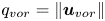 $q_{vor}= \|{\boldsymbol u}_{vor}\|$, a self-inducing co-rotating pair would be characterised by
 $q_{cg}\ll q_{pair}\equiv (q_A+q_B)/2$, while a dipole would satisfy
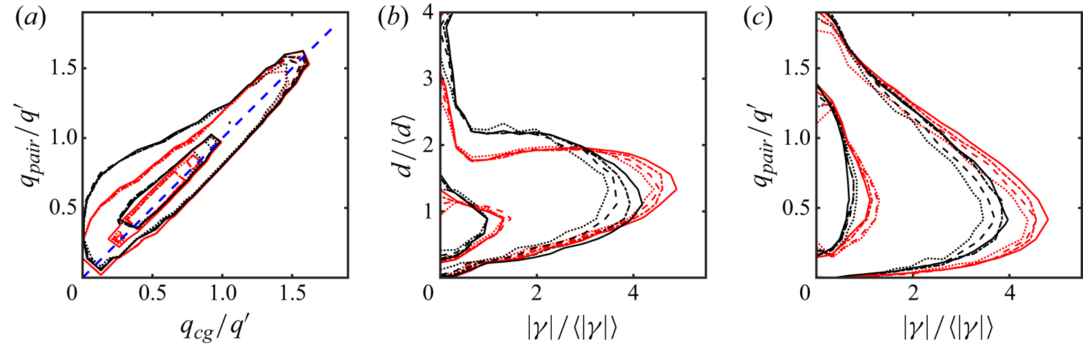
 $q_{cg}\approx q_{pair}$. This is tested in figure 10(a), and it is only satisfied by slow-moving vortices. The behaviour of fast pairs for which
 $q\gtrsim q'$ is independent of whether they are co- or counter-rotating, and they can therefore be assumed to be mostly advected by a background velocity field.
Properties of the vortex pairs. (a) Joint p.d.f. of the velocity of the centre of gravity of a vortex pair versus the averaged velocity magnitude of its two component vortices. In all the panels in this figure:  , T256;
 , T512;
 , T768;
 , T1024. Red lines are dipoles, and black ones are co-rotating pairs. The two probability contours in each case enclose 50 % and 95 % of the probability mass. (b) Mean circulation magnitude of the vortex components of the pair, versus the inter-component distance. (c) Vortex circulation versus vortex mobility.

Figure 10(b) shows that vortex pairs can be classified into two groups. The ‘nose’ extending to the lower right in the figure represents a family of strong cores with large circulations, whose intra-pair distance is relatively small. This family exists for co-rotating pairs and for dipoles, although it is most marked for the latter. The vertical band to the left of the figure contains relatively weak vortices with no clear preference for a particular coupling distance. Most vortex pairs are in this latter family, but they are relatively unimportant for the flow. Approximately 66 % of the cores have  $|\gamma |<\langle |\gamma |\rangle$, but they only contain 15–25 % of the total circulation magnitude. A similar distinction can be based on vortex area (not shown), since the mean vorticity is relatively uniform among the vortices. The classification into vortex types can be based on either property.
One could hypothesise that the large, tightly coupled vortices in the ‘nose’ family would be the ones with the fastest mobilities, which they would induce on each other, but figure 10(c) shows that the opposite is true. The vortices with the largest circulations move relatively slowly, and the high mobilities tend to be associated with the weak circulations to the left of the figure. This somewhat surprising observation leads to a model in which a set of organising large vortices in an ‘approximate equilibrium’ configuration are responsible for organising the flow into streams where weaker vortices are advected at relatively high speed.
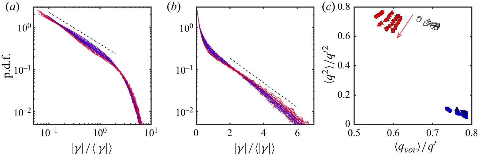
In fact, the large and small vortices have very different properties. Figure 11(a,b) shows the one-dimensional p.d.f. of the core circulation, which collapses reasonably well for all the simulations and evolution times. Figure 11(a) shows that the weak vortices,  $|\gamma |< \langle |\gamma |\rangle$, follow a power-law distribution
 $P(|\gamma |)\sim |\gamma |^{-3/4}$, while figure 11(b) shows that the vortices above that limit follow an exponential one. The separation of decaying two-dimensional turbulence into coherent vortices evolving under mutual induction, and a ‘chaotic’ background has been discussed often (Benzi et al. Reference Benzi, Patarnello and Santangelo1987; Benzi, Patarnello & Santangelo Reference Benzi, Patarnello and Santangelo1988; McWilliams Reference McWilliams1990b), but the background is usually not characterised in term of vortices, and we are not aware of any previous characterisation of the larger vortices as slowly moving. For example, Benzi et al. (Reference Benzi, Patarnello and Santangelo1987) discuss the large vortices as the only coherent structures in the flow and report that their areas follow a power-law distribution, although with a different exponent than the one above,
 $|\gamma | ^{-3/2}$. The reason for this difference is not clear, but we mentioned in § 2 that Benzi et al. (Reference Benzi, Patarnello and Santangelo1987) study a later stage of the decay, and that they use a higher-order viscous dissipation, which presumably creates different vortex cores (McWilliams Reference McWilliams1990b; Jiménez Reference Jiménez1994). It is also unclear why the exponential range of the distribution in figure 11(b) is not discussed by Benzi et al. (Reference Benzi, Patarnello and Santangelo1987), although this may be partly due to their different sample size. The analysis in their paper is based on 17 vortices, while each of the distributions in figure 11 represents
 $10^4$–
 $10^5$ objects.
(a) Probability density function of the vortex circulation magnitude. In all cases, time increases from blue to red. The dashed line is proportional to  $|\gamma |^{-0.75}$. (b) As in (a). The dashed line is proportional to
 $\exp (-0.666 |\gamma |/ \langle |\gamma |\rangle )$. (c) Kinetic energy contained in different vortex classes versus mean vortex mobility. Open symbols are all the thresholded vortices; red symbols are large vortices,
 $s_{vor} \ge \langle s_{vor}\rangle$; blue symbols are
 $s_{vor} < \langle s_{vor}\rangle$. The red arrow is the direction of time advance for the red symbols.

Figure 11(c) shows that the kinematics of the weak and strong cores is very different. The vertical axis in this figure is the fraction of the kinetic energy carried by the thresholded vortices, defined as in figure 9(i). The open symbols are the contribution from all the vortices, as in that figure, and the red symbols are the contribution from vortices whose area is larger than the average. They contain most of the kinetic energy. The blue symbols in the lower-right corner are the contribution from vortices smaller than the average, which is much smaller. The horizontal axis is the average vortex mobility defined as the modulus of (4.1). The large and small vortices lie in very different parts of the plot, as already suggested by figure 10(c). Large vortices are responsible for most of the kinetic energy of the flow, but are themselves relatively immobile, while small ones move fast, but are only responsible for a small fraction of the kinetic energy.
The power-law and exponential probability distributions suggest that the cores grow by two different aggregation mechanisms of smaller units. While a power law implies self-similar scale-free growth, in which cores merge with other cores of similar size (Benzi et al. Reference Benzi, Colella, Briscolini and Santangelo1992), an exponential has a definite scale, which is proportional to the mean of the distribution, and to the size of the elements being accreted (Jiménez & Kawahara Reference Jiménez, Kawahara, Davidson, Kaneda and Sreenivasan2013). In figure 11 the lower limit of the exponential is indeed of the order of  $\langle |\gamma |\rangle$, and it is interesting to speculate about an aggregation model in which cores merge self-similarly with each other until they grow to be large enough to ‘freeze’ in a quasi-equilibrium slowly evolving pattern. The motion of these large vortices is not chaotic, at least over short times, and these cores stop merging among themselves. But they keep absorbing the remaining fast-moving vortices of the background, and the largest of these field vortices determine the scale of the exponential distribution.
Over a much longer time scale, it is to be expected that even the ‘frozen’ vortices would merge among themselves, in an amalgamation process similar to the one described by Carnevale et al. (Reference Carnevale, McWilliams, Pomeau, Weiss and Young1991, Reference Carnevale, McWilliams, Pomeau, Weiss and Young1992), but the appearance of a collective equilibrium signals that the energy scale has become of the order of the box size. As mentioned in § 2, this is the limit of our simulations, and of the analysis in this paper.
Vortex arrangements that remain stationary in some frame of reference have been studied for over a century (see the review in Aref et al. Reference Aref, Newton, Stremler, Tokieda and Vainchtein2002). Some of them are stable, and form spontaneously in experiments. In particular, forced two-dimensional turbulence is known to settle to stationary vortex ‘crystals’ which are partly determined by the forcing method and by the boundary conditions (Fine et al. Reference Fine, Cass, Flynn and Driscoll1995; Jin & Dubin Reference Jin and Dubin2000; Jiménez & Guegan Reference Jiménez and Guegan2007), and beautiful examples of equilibrium vortex polygons have been observed in the polar regions of planetary atmospheres (Tabataba-Vakilia et al. Reference Tabataba-Vakilia, Rogers, Eichstädt, Orton, Hansen, Momary, Sinclair, Giles, Caplinger and Ravine2020). Most known equilibrium systems are regular arrangements of vortices of a single sign in a background of opposite-sign vorticity, but mixed-sign stable systems are also known. The von Kármán vortex street is probably the best known example of the latter, and it is known that two-dimensional turbulence in a square box converges to a quasi-equilibrium single dipole, arranged diagonally in the box, which only decays slowly by viscosity (Smith & Yakhot Reference Smith and Yakhot1993).
The circulation of the slow-moving vortices discussed here is essentially in balance (with a residue of 1 %–3 % of  $\omega '$), but they are still far from equilibrium, and may perhaps be considered an intermediate stage to a final steady state. Attempts to extract a regular arrangement for them failed, beyond the four-way symmetry induced by the computational box, but the drop in mobility can be considered diagnostic of incipient ‘crystallisation.’
4.2. The up-scale energy flux
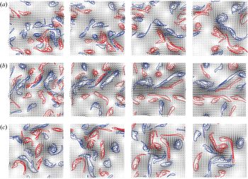
The discussion in the previous section raises the question of how the dipoles get organised into long streams. Three examples are given in figure 12. These examples were chosen for didactic purposes to demonstrate the aggregation process, and are not truly random. But they are fairly representative. Of the several thousand simulations available, approximately 30 % were found visually to display an initial evolution similar to those in the figure. Three of those were chosen at random from about 50 ‘good’ cases. Each row in the figure is a simulation, displayed at four approximately equidistant times, which are the same for the three cases. Vortices are represented in colour, according to their sign, and the arrows are the velocities. The intensity of the grey background is the velocity magnitude. To best display the evolution, only the largest vortices  $(s>\langle s\rangle )$ are included in each plot, and the Reynolds number is purposely chosen low.
Three examples of the organisation of vortices into streams. Time runs in each row from left to right,  $\omega _0't=0$, 2, 4.6, 6.5. Case T256. The three rows are independent realisations, and only vortices with
 $s>\langle s \rangle$ are included in the figure. Line contours are positive (red) and negative (blue) vorticity, the arrows are velocity, and the grey background is the velocity magnitude.

Each simulation starts with a relatively disorganised arrangement of vortices but, at the end of each sequence, positive (red) vortices have sorted themselves to one side of the flow, and negative (blue) ones to the other, supporting a jet between them. Some merging of like-signed vortices takes place in all cases.
The question is how this happens, because, while continuity probably implies that the velocity of any elongated velocity structure should be aligned with its axis, the opposite is not true. Compact jet-like vortex dipoles with aspect ratios of order one (modons) are well-known stable solutions of the Euler and Navier–Stokes equations (Flierl et al. Reference Flierl, Larichev, McWilliams and Reznik1980; McWilliams Reference McWilliams1980).
Simulations of point vortex systems (not shown) spontaneously form tight dipoles and co-rotating pairs, but the dipoles do not organise into trains or jets, as is the case in figure 12(a,b). Neither do they form stronger dipoles of vortex ‘clouds,’ as in figure 12(c). When a point dipole collides with a solitary point vortex or with a co-rotating pair, it often loses one of its vortices, possibly breaking the colliding couple and forming a new association. Very seldom the resulting arrangement involves more than two vortices.
Of course, sets of point vortices are Hamiltonian systems whose interactions conserve energy (Batchelor Reference Batchelor1967). Both the merging of like-signed vortices and the breaking of an existing dipole involve energy exchanges, which are much simpler if viscosity or filamentation can be used as an energy dump. This would statistically favour the formation of the lower-energy dipoles, but any such selection criterion requires a local mechanism to implement it. In particular, it is unclear why a positive vortex being overtaken by a dipole would tend to reinforce the positive component of the dipole, strengthening it, rather than merging with the negative one, weakening it.
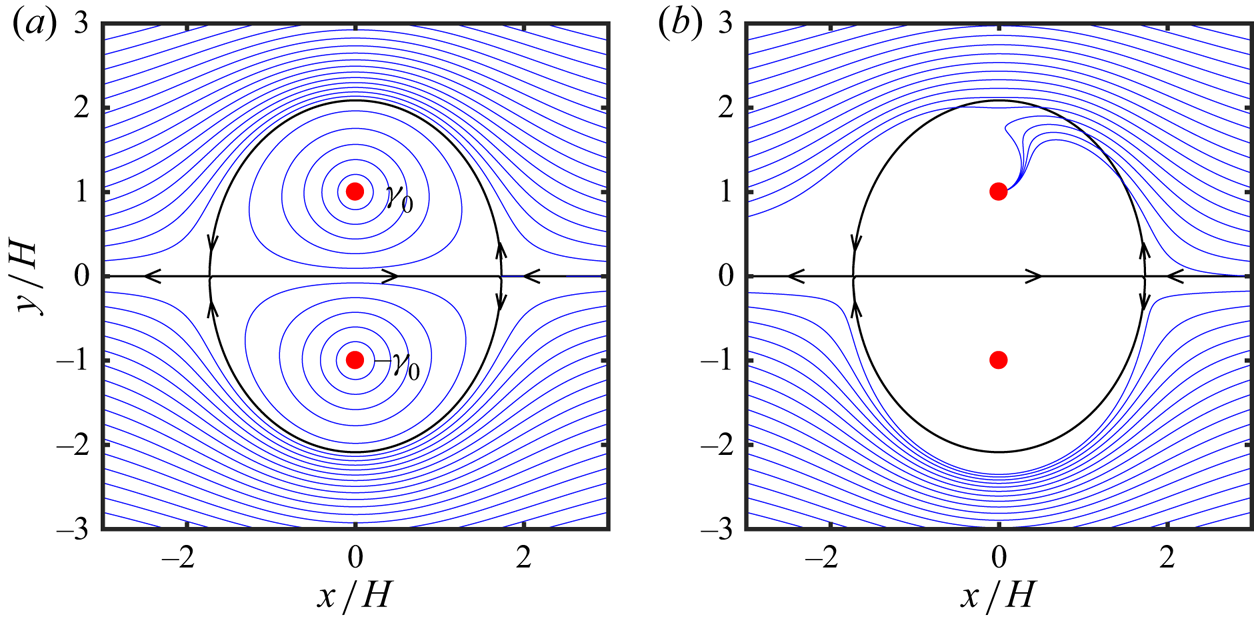
A possible mechanism is explained in figure 13. Consider the point vortex dipole in figure 13(a). In the comoving frame of reference, it forms a recirculation bubble separated from infinity by an approximately elliptical dividing streamline (see appendix B). Any sufficiently weak point vortex being overtaken by the dipole follows the streamlines around the bubble, independently of its sign, and it is eventually left behind. There is no preference for which side of the dipole its path takes, and it is therefore unlikely to statistically strengthen or weaken it.
(a) Velocity field of a dipole of equal point vortices of circulation  $\pm \gamma _0$ at distance
 $2H$. The dipole is moving to the right, but is shown in the frame of reference linked to the vortices. The blue lines are streamlines, as well as the trajectories of an advected point vortex. The black lines are the dividing streamline in this frame of reference. (b) As in (a), but the blue lines are the trajectories of the centre of gravity of a vortex patch of positive circulation
 $\gamma$ and area
 $s$, such that
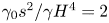 $\gamma _0 s^2/\gamma H^4=2$. A patch with negative circulation would be entrained to the negative vortex in the dipole. Only trajectories coming from large positive
 $x$ are included. See text and appendix B for details.

The situation is different for the entrainment of an extended vortex, as detailed in appendix B for the case of a uniform vortex patch. Such patches drift with respect to the advecting streamlines, as shown by the trajectories in figure 13(b). Positive patches drift towards the positive component of the dipole, and negative ones towards the negative component. The result is an average strengthening of the dipole, and the formation of organised jets.
Note that this accretion model could explain the asymmetry observed in figure 8, where it was shown that the direction of the velocity of a stream is a better predictor of the direction taken by the stream ahead than behind the position at which it is measured. In the model presented here dipoles propagate forward, and take some time to incorporate new vorticity. The jet of a growing dipole is strongest at its trailing edge, and, therefore, predicts better the position of the leading dipole ahead of it. Examples of this asymmetry between the front and back of dipoles can be seen in figures 12(a) and 12(c), where a growing head dipole is followed by a trailing jet of elongated filaments that have been created during their interaction with the dipole.
On the other hand, although accretion explains why existing dipoles become stronger, and thus how they segregate into classes, it does not explain how they organise into longer streams. Several examples of both processes can be seen in figure 12. For example, the flow in figure 12(c) organises into a single strong dipole but not into a long stream. Figure 12(b) forms a horizontal leftwards jet in the middle of the frame, but none of its dipoles is especially strong, and the same is true of the oblique jet forming in the lower-right corner of figure 12(a). The growth of the longitudinal scale in a set of two-dimensional vortices first came under consideration when modelling the spreading of free shear layers in Brown & Roshko (Reference Brown and Roshko1974). Two mechanisms were proposed at the time. In ‘vortex pairing’ two vortices of the same sign merge into a larger one (Winant & Browand Reference Winant and Browand1974), while in ‘vortex tearing’ a weaker vortex between two stronger ones is strained into a filament that is eventually entrained or dissipated (Moore & Saffman Reference Moore and Saffman1975). The accretion model developed above can be considered a case of pairing, and a clear tearing can be seen between the second and third frames of figure 12(b). Both processes are relevant in experimental shear layers (Hernán & Jiménez Reference Hernán and Jiménez1982), but that flow involves vorticity of a single sign, and the scale growth mostly takes place along a single axis. Repeating a similar analysis in the present mixed-sign isotropic situation would involve a more thorough processing than is possible here, both theoretically and observationally.
The interaction of fast-moving dipoles with smaller vortices, akin to tearing, has been invoked by Dritschel et al. (Reference Dritschel, Scott, Macaskill, Gottwald and Tran2008) as an important step of the forward enstrophy cascade. It takes place when a third vortex is shredded by a dipole, but, to our knowledge, such interactions have not been connected with the up-scale cascade. In a related observation, random forcing of two-dimensional turbulence induces a self-similar enstrophy cascade, but the cascade disappears (to form vortex crystals) when the forcing is partially deterministic, and the character of the flow again changes when the forcing is fully deterministic, in which case the flow becomes a ‘dilute gas of dipoles’ that cleans most of the background low-level vorticity (Jiménez & Guegan Reference Jiménez and Guegan2007).
5. Discussion and conclusions
We have used simulation ensembles of decaying two-dimensional turbulence to study the early stages of the evolution of the flow from a disorganised state towards a set of vortex cores and large-scale structures of the kinetic energy. In this period, the dominant scale of the kinetic energy is still small compared to the size of the computational box, and grows monotonically. We have shown that, at least at the moderate Reynolds numbers of our simulations, this growth is due to the appearance of elongated ‘streams’ formed by a concatenation of vortex dipoles. The growth of the energy scale is not due to the elongation of the streams, whose aspect ratio stays in the range of 8–10, but to their proliferation, and to the increase of the area fraction that they cover.
We have shown that the formation of the streams includes a process of aggregation of the vortex cores. The cores segregate into two separate classes. Most of them are small and mobile, and merge among themselves in a self-similar cascade that results in a power-law probability distribution of vortex sizes (Benzi et al. Reference Benzi, Colella, Briscolini and Santangelo1992). A few of the cores grow larger, and eventually ‘freeze’ into a low-mobility vortex system. These larger vortices are responsible for most of the kinetic energy of the flow, but they themselves move slowly, in what can be described as a quasi-equilibrium vortex ‘crystal.’ The probability distribution of their areas and circulations is exponential, rather than a power law, suggesting that they do not grow by interacting among themselves, at least in the time scales considered here, but by absorbing smaller vortices from the self-similar background. They are responsible for the formation of the streams. We have proposed a formation mechanism by noting that, although a vortex dipole shows no preference about how to entrain a point vortex of either sign, the drift velocity of vortex patches biases positive patches to merge with the positive component of the dipole, and negative ones to merge with the negative component. As a consequence, the dipoles are strengthened and the streams are formed.
This growth mechanism of the energy scale is probably not the classical inverse energy cascade, which is typically observed in forced, rather than in decaying flows. There are two main properties that have to be explained for this cascade (Tabeling Reference Tabeling2002; Boffetta & Ecke Reference Boffetta and Ecke2012). The first one is its  $k^{-5/3}$ power spectrum, and the second one is its low intermittency. The latter is consistent with the processes discussed here, because growth by aggregation of small units of fixed size is an additive process, which is not intermittent. But the observed exponential probability distribution of the vortex size, and the approximately crystallisation, argue against the self-similarity implied by a power spectrum. Note that there is no
 $k^{-5/3}$ plateau in the spectral slopes in figure 1(c). It is possible that the aggregation of dipoles into streams is hierarchical and self-similar in much larger simulations, but it is difficult to see how such a self-similar amalgamation could avoid producing intermittency (Frisch, Sulem & Nelkin Reference Frisch, Sulem and Nelkin1978). Moreover, the facility with which streams are formed in figure 12, suggests that it would be hard to prevent the large-scale vortex organisation from falling into local equilibrium. A more appealing possibility is that the reason why a self-similar inverse cascade is only observed in forced flows is that the effect of the forcing is to locally ‘melt’ the vortex crystal, much as a liquid develops short-range order and long-range disorder. Although analysing such a model is beyond the scope of the present paper, a process of repeated short-range crystallisation and longer-range melting caused by random excitations, is probably not particularly intermittent. We mentioned above that partially deterministic forcing can inhibit the forward enstrophy cascade (Jiménez & Guegan Reference Jiménez and Guegan2007), but, to our knowledge, no systematic study of the effect of forcing on the inverse cascade is available.
It is difficult not to be reminded by the discussion above of other examples of spontaneous stream formation in more complicated flows. The best known are probably the streaks in wall-bounded turbulence and other shear flows (Tsukahara, Kawamura & Shingai Reference Tsukahara, Kawamura and Shingai2006; Dong et al. Reference Dong, Lozano-Durán, Sekimoto and Jiménez2017; Jiménez Reference Jiménez2018a), and the azimuthal jets of planetary atmospheres and rotating flows (Maltrud & Vallis Reference Maltrud and Vallis1991; Dritschel & McIntyre Reference Dritschel and McIntyre2008; Grossmann, Lohse & Sun Reference Grossmann, Lohse and Sun2016; Sacco, Verzicco & Ostilla-Mónico Reference Sacco, Verzicco and Ostilla-Mónico2019). In many of these cases, the streams are a streamwise concatenation of smaller units (Lozano-Durán, Flores & Jiménez Reference Lozano-Durán, Flores and Jiménez2012), and the question arises of how these units organise longitudinally. This is not the place to review the many models proposed for this organisation, but most of them depend on the generation of new vorticity, which is readily available from the shear or from the planetary rotation. There is no vorticity generation in a two-dimensional flow, and the mechanism discussed here, which depends on the reorganisation of vorticity rather than on its creation, suggests that some of these streams may, at least in part, share a common mechanism which is more related to symmetry breaking and pattern formation (Cross & Greenside Reference Cross and Greenside2009) than to the dynamics of the energy-generation process.
It is finally interesting to remark that, although the analysis in this paper is a fairly classical example of hypotheses-driven research, it was made possible by following the ‘blind suggestion’, from the Monte–Carlo experiments in Jiménez (Reference Jiménez2020b), that dipoles are at least as relevant to two-dimensional turbulence as individual vortex cores. Hypothesis-driven science is, of course, the standard scientific method, and it can be argued to be the only way in which the scientific corpus derives new ‘theories’ from the empirical accumulation of facts (Poincaré Reference Poincaré1920). A different question is how the hypotheses to be tested are chosen, and, preferably but not necessarily, whether the resulting ‘theory’ can be related back to this choice. In the present case, the original intriguing observation was that dipoles of relatively small size had global effects (Jiménez Reference Jiménez2020b), and it can easily be explained from the results of the subsequent analysis: killing a dipole amounts to blocking a stream, and has effects over the length of the stream. The mismatch between the size of the cause and of the effect is the elongation of the object being modified. In a sense, the initial Monte-Carlo search is being used here as a ‘hypothesis generator’, while the rest of the paper is the ‘hypothesis test’, and it is tempting to speculate that this could be a reasonable division of labour between computer and researcher. Further discussion of these ‘epistemological’ issues can be found in Jiménez (Reference Jiménez2020a,Reference Jiménezb).
Acknowledgements
This work was supported by the European Research Council under the Coturb grant ERC-2014.AdG-669505.
Declaration of interests
The authors report no conflict of interest.
Appendix A. Poisson distribution of the closest point
If the expected number of Poisson-distributed points in a set parametrised with  $r$ is
 $\lambda (r)$, the probability of finding no points within the set is
 \begin{equation} P_0(r) = \exp(-\lambda), \end{equation}
and the probability density that the first point is precisely at  $r$ is
 \begin{equation} P_c(r) = -(\textrm{d} P_0/\textrm{d} r) = (\textrm{d} \lambda/\textrm{d} r) \exp(-\lambda). \end{equation}
For a set of points distributed in a plane with uniform average density  $\rho$, the expected number of points within a distance
 $r$ of a reference position is
 $\lambda ={\rm \pi} \rho r^2$, and
 \begin{equation} P_c(r) = 2{\rm \pi}\rho r \exp(-\rho {\rm \pi}r^2 ). \end{equation}
This distribution can be integrated to show that the average distance to the closest point is 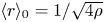 $\langle r\rangle _0 = 1/\sqrt {4\rho }$, so that (A 3) can be written as
 \begin{equation} P_c(\xi) = ({\rm \pi}\xi/2) \exp(-{\rm \pi} \xi^2/4), \end{equation}
where  $\xi =r/\langle r \rangle _0$.
If we add the restriction that no point can be closer than a distance  $a$ (e.g. the vortex diameter), the expected number of points within a distance
 $r\ge a$ is
 $\lambda ={\rm \pi} \rho (r^2-a^2)$,
 \begin{equation} P_c(r) = 2{\rm \pi}\rho r \exp[-\rho {\rm \pi}(r^2-a^2) ], \end{equation}
and the average distance to the closest point becomes
 \begin{equation} \langle r\rangle_\epsilon = \int_a^\infty r P_c(r) \,\textrm{d} r = a +(1/2\sqrt{\rho}\,) {{\rm erfc}} (\epsilon) \exp(\epsilon^2),\end{equation}
where  $\epsilon =a/\sqrt {\rho {\rm \pi}}=\sqrt {4/{\rm \pi} }a/\langle r \rangle _0$. It can be shown that
 $\langle r\rangle _\epsilon \approx a$ for
 $\epsilon \gg 1$, but that
 $\langle r\rangle _\epsilon \approx \langle r\rangle _0$ for
 $\epsilon \lesssim 0.5$. Figure 9(e) suggests that
 $\hat {a}=a/\langle r \rangle _0\approx 0.2\text {--}0.3$, so that
 \begin{equation} P_c(\xi) \approx ({\rm \pi}\xi/2) \exp[-{\rm \pi} (\xi^2-\hat{a}^2)/4],\quad \xi>\hat{a}. \end{equation}
The effect is to crop the part of the distribution near the origin, while raising its peak to compensate for the missing mass (as in figure 1e).
Appendix B. Drift of a vortex patch
While point vortices are advected by the flow velocity, vortices with a wider support drift with respect to it. In the particular case of small patches of uniform vorticity, the drift velocity can be computed as a series expansion of the vortex radius. The following equations of motion are drawn from Jiménez (Reference Jiménez1988).
Define a complex variable  $z=(x+\textrm {i} y)/H$, where
 $H$ is a characteristic length scale, and consider a uniform vortex patch of circulation
 $\gamma \varGamma$ and area
 $s$. Using
 $\varGamma$ and
 $H$ to define the time and length scales, the expansion parameter is
 $\epsilon ^2=s/{\rm \pi} H^2$, which is assumed to be small. The irrotational complex flow velocity in the absence of the patch is described by an analytic function
 $w_\infty (z)= (u-\textrm {i} v)H/\varGamma$, with a similar non-analytic expression within the patch. To lowest order, the contour of the patch is an ellipse,
 \begin{equation} z-z_c = \epsilon\eta (1+b_2 \epsilon^2/\eta^2), \end{equation}
where  $z_c$ is the centre of gravity of the patch, and
 $\eta =\exp (\textrm {i} \phi )$ is the unit circle. Matching at this contour the expansions of the velocity inside and outside the patch provides an evolution equation for the ellipticity,
 \begin{equation} 2{\rm \pi}\epsilon^2 \,\textrm{d} b_2/\textrm{d} \tau = \textrm{i} \gamma b_2 +c_2^*, \end{equation}
where  $\tau =\varGamma t/H^2$ is a rescaled time, the asterisk stand for complex conjugation, and
 \begin{equation} c_k = \frac{2{\rm \pi}}{(k-1)!}\frac{\textrm{d}^{k-1} w_\infty}{\textrm{d} z^{k-1}}(z_c). \end{equation}
The drift velocity, defined as  $\textrm {d} z^*_c/\textrm {d} \tau = w_\infty (z_c)+w_d$, can be expressed as
 \begin{equation} w_d= (\epsilon^4/2{\rm \pi}) b_2 c_3, \end{equation}
and, if we further assume that (B 2) has reached equilibrium, so that  $b_2= \textrm {i} c_2^*/\gamma$,
 \begin{equation} w_d = \frac{{\rm \pi}\textrm{i} \epsilon^4 }{\gamma} \frac{\textrm{d} w^*_\infty}{\textrm{d} z^*}\frac{\textrm{d}^2 w_\infty}{\textrm{d} z^2}. \end{equation}
Consider now the effect on the patch from a dipole formed by two point vortices of circulation  $\varGamma \gamma _0$ separated by a distance
 $2H$. In figure 13(a) in the body of the paper, the positive vortex is on top, and the dipole would move to the right, but it is made stationary by a uniform negative velocity at infinity. Consider a third vortex being overtaken by the dipole, but neglect its effect on the dipole itself. In the units defined above, the velocity induced by the dipole is
 \begin{equation} w_\infty = \frac{\gamma_0}{\rm \pi} \left( \frac{1}{1+z^2}-\frac{1}{4}\right). \end{equation}
Its effect on a point vortex is given by the streamlines in figure 13(a). The vortex is deflected around the recirculation bubble of the dipole, and eventually left behind. There is no difference between a positive and a negative vortex, but the situation is different for an extended patch, because the drift velocity,
 \begin{equation} w_d = - \frac{4\textrm{i}\gamma_0^2\epsilon^4}{\gamma{\rm \pi}} \frac{z^*}{1+z^{*2}}\frac{3z^2-1}{(1+z^2)^3}, \end{equation}
depends on the sign of the circulation of the patch being overtaken. As shown in figure 13(b), positive vortices tend to be entrained into the upper part of the stream, and to merge with the positive vortex of the dipole. Negative patches are entrained towards the lower negative vortex. The result is that the dipole is reinforced on average.