1. Introduction
The dual conservation of kinetic energy (KE) and enstrophy in two-dimensional (2D) incompressible Euler flow gives rise to an inverse cascade in which KE moves to large scales, while enstrophy moves to small scales in a direct cascade (Kraichnan Reference Kraichnan1967; Batchelor Reference Batchelor1969). Two-dimensional Euler flow belongs to a family of fluid models referred to as generalized 2D fluids, also known as
 ${\it\alpha}$
-turbulence models (Pierrehumbert, Held & Swanson Reference Pierrehumbert, Held and Swanson1994), which all possess two quadratic invariants leading to dual inverse and direct cascades. In generalized 2D fluids an active scalar
 ${\it\theta}$
is advected by a velocity field to which it is functionally related,
 ${\it\theta}=(-{\it\Delta})^{{\it\alpha}/2}{\it\psi}$
, where
 ${\it\psi}$
is the streamfunction and
 ${\it\alpha}$
is a parameter controlling the scale separation between
 ${\it\psi}$
and
 ${\it\theta}$
. For
 ${\it\alpha}>0$
the dynamics should become more spectrally nonlocal as
 ${\it\alpha}$
increases. When
 ${\it\alpha}=2$
, the active scalar is the familiar vorticity
 ${\it\omega}=-{\rm\nabla}^{2}{\it\psi}$
, where we use Batchelor’s sign convention (Batchelor Reference Batchelor1969), and the system reduces to 2D Euler flow as a special case. Strongly rotating quasigeostrophic flows (Pedlosky Reference Pedlosky1987) and plasmas in strong magnetic fields (Hasegawa & Mima Reference Hasegawa and Mima1978) both correspond to
 ${\it\alpha}=-2$
, while surface quasigeostrophic dynamics (SQG) corresponds to
 ${\it\alpha}=1$
. Hence generalized 2D fluids are physically relevant as well as allowing one to explore how varying spectral nonlocality affects 2D turbulence.
The extent to which Kraichnan–Leith–Batchelor (KLB) similarity theory (Kraichnan Reference Kraichnan1967; Leith Reference Leith1968; Batchelor Reference Batchelor1969) describes inverse cascades is a major unresolved issue in 2D turbulence. Similarity theory, which assumes scale-invariant inertial ranges in which transfers are spectrally local, predicts that the generalized energy spectrum
 $\mathscr{E}(k)$
follows a power law
 $\mathscr{E}(k)\propto k^{-(7-{\it\alpha})/3}$
in the inverse cascade. For
 ${\it\alpha}=2$
this yields the well-known
 $-5/3$
law for the KE spectrum. For
 ${\it\alpha}\geqslant 2$
the strain rate in the direct cascade becomes nonlocally dominated and KLB theory simultaneously fails (Kraichnan Reference Kraichnan1971; Watanabe & Iwayama Reference Watanabe and Iwayama2004), which is not surprising because KLB theory assumes spectral locality. In the inverse cascade local contributions are expected to dominate the strain rate for
 ${\it\alpha}<4$
, which led previous authors (Pierrehumbert et al.
Reference Pierrehumbert, Held and Swanson1994; Smith et al.
Reference Smith, Boccaletti, Henning, Marinov, Tam, Held and Vallis2002) to conclude that the inverse cascade would be spectrally local for
 ${\it\alpha}<4$
, in which case one expects KLB theory to apply. However, generalizing the eddy damped quasinormal Markovian (EDQNM) closure to
 ${\it\alpha}$
turbulence, Burgess & Shepherd (Reference Burgess and Shepherd2013) showed that the KLB similarity solutions are associated with vanishing energy flux for
 ${\it\alpha}=2.5$
and downscale flux for
 ${\it\alpha}>2.5$
. On the basis of this, they predicted that the KLB spectrum would not be observed for
 ${\it\alpha}\geqslant 2.5$
. This was confirmed by low-resolution simulations forced in the dissipation range, thereby suppressing the formation of coherent vortices, which exhibited the KLB spectrum for
 ${\it\alpha}<2.5$
but not
 ${\it\alpha}\geqslant 2.5$
.
Despite the archetypal status of the inverse KE cascade for
 ${\it\alpha}=2$
, there is disagreement about its phenomenology and statistical characteristics. Some authors, e.g. Boffetta & Ecke (Reference Boffetta and Ecke2012), claim that this cascade is well described by self-similar inertial range theory, lacks coherent vortices, has almost Gaussian statistics, and is non-intermittent. The
 $k^{-5/3}$
scaling has been observed in a number of numerical simulations (Frisch & Sulem Reference Frisch and Sulem1984; Maltrud & Vallis Reference Maltrud and Vallis1991; Boffetta, Celani & Vergassola Reference Boffetta, Celani and Vergassola2000; Dubos et al.
Reference Dubos, Babiano, Paret and Tabeling2001; Bruneau & Kellay Reference Bruneau and Kellay2005; Boffetta Reference Boffetta2007) and laboratory experiments (Sommeria Reference Sommeria1986; Paret & Tabeling Reference Paret and Tabeling1998; Rutgers Reference Rutgers1998; Dubos et al.
Reference Dubos, Babiano, Paret and Tabeling2001; Bruneau & Kellay Reference Bruneau and Kellay2005), leading some authors to posit that the inverse cascade is ‘more robust’ than the enstrophy cascade (Paret & Tabeling Reference Paret and Tabeling1998), which in numerous simulations exhibits slopes significantly steeper than the KLB prediction (Basdevant, Legras & Sadourny Reference Basdevant, Legras and Sadourny1981; McWilliams Reference McWilliams1984; Babiano et al.
Reference Babiano, Basdevant, Legras and Sadourny1987; Santangelo, Benzi & Legras Reference Santangelo, Benzi and Legras1989).
However, most of the studies that found
 $k^{-5/3}$
scaling in the inverse KE cascade used forcing near the largest resolved wavenumber, which does not allow an enstrophy cascade to develop, and/or a large-scale drag or hypoviscosity. Smith & Yakhot (Reference Smith and Yakhot1994) attributed almost Gaussian statistics and a
 $k^{-5/3}$
scaling to the fact that no enstrophy cascade was present in their simulations. They argued that when the enstrophy range is absent nonlinear interactions between
 $k<k_{f}$
and
 $k>k_{f}$
are minimized, where
 $k_{f}$
is the forcing wavenumber. The small-scale dynamics are then dominated by the random forcing rather than by nonlinearity, and this results in an almost Gaussian inertial range with
 $k^{-5/3}$
scaling. Similarly, large-scale drag can disrupt the formation of coherent structures, although Elhmaidi (Reference Elhmaidi2005) also found that it could lead to filament instability and vortex formation; the effect of hypoviscosity is thus not clear, and perhaps variable depending on the particular parameters of the simulation.
Other studies have found spectra significantly steeper than
 $k^{-5/3}$
in the inverse KE cascade, suggesting the KLB scaling is not generic (Borue Reference Borue1994; Smith & Yakhot Reference Smith and Yakhot1994; Danilov & Gurarie Reference Danilov and Gurarie2001; Scott Reference Scott2007; Bos & Bertoglio Reference Bos and Bertoglio2009; Vallgren Reference Vallgren2011; Fontane, Dritschel & Scott Reference Fontane, Dritschel and Scott2013). Borue (Reference Borue1994) found spectra close to
 $k^{-3}$
; filtering out the vortices showed that the incoherent background field still exhibited the
 $k^{-5/3}$
scaling, and that the spectrum associated with the vortices was steeper. Scott (Reference Scott2007) studied the inverse KE cascade in the quasi-stationary state, i.e. with no large-scale friction, and found that when
 $\mathit{Re}=k_{max}^{2}/k_{f}^{2}$
exceeded a threshold such that a direct enstrophy cascade developed, the spectrum in the inverse energy cascade steepened from
 $k^{-5/3}$
to
 $k^{-2}$
; this is consistent with Smith and Yakhot’s argument that nonlinear interactions at small scales are suppressed when an enstrophy cascade is not present. Fontane et al. (Reference Fontane, Dritschel and Scott2013) obtained a similarly steep
 $k^{-2}$
spectrum in an ensemble average of quasi-stationary simulations using the combined Lagrangian advection method; they also found that energy grew like
 $t^{-1}$
at large scales, where
 $t$
is time, in contrast with Kraichnan’s predicted
 $t^{-3/2}$
growth rate (Kraichnan Reference Kraichnan1967).
Two studies (Farazmand, Kevlahan & Protas Reference Farazmand, Kevlahan and Protas2011; Mizuta, Matsumoto & Toh Reference Mizuta, Matsumoto and Toh2013) have demonstrated that the spectral scaling in the inverse KE cascade and the emergence of vortices depend not only on the simulation parameters but also the form of the forcing. Farazmand et al. (Reference Farazmand, Kevlahan and Protas2011) found that dual cascades satisfying the KLB scaling only formed in response to an optimal forcing unlikely to be spontaneously realized. Mizuta et al. (Reference Mizuta, Matsumoto and Toh2013) found that coherent structures formed in response to a random forcing, while deterministic forcing resulted in no vortices and a
 $k^{-5/3}$
spectrum.
A recent review of turbulence (Boffetta & Ecke Reference Boffetta and Ecke2012) attributed the steeper inverse KE cascade spectra found by Borue (Reference Borue1994), Danilov & Gurarie (Reference Danilov and Gurarie2001) and Bos & Bertoglio (Reference Bos and Bertoglio2009) to strong hypoviscosity causing effects mimicking Bose condensation. However, as already shown by Scott (Reference Scott2007), Vallgren (Reference Vallgren2011) and Fontane et al. (Reference Fontane, Dritschel and Scott2013), spectra steepen even in the absence of hypoviscosity, as long as the forcing scale is well resolved and there is an enstrophy cascade present. The steepening found by these authors cannot be attributed to Bose condensation or hypoviscosity effects mimicking condensation, so another explanation must be sought; as evidenced by filtering the vorticity field, the likely culprit is coherent vortices, which form unless nonlinear interactions around the forcing scale are suppressed by inadequate resolution.
Somewhat relatedly, the degree to which the inverse KE cascade is intermittent and non-Gaussian is unsettled, with contradictory results reported. Intermittency arises when spectral transfers and/or dissipation are not space filling, and the measure of their spatial support varies with scale. If the turbulence is intermittent, its statistics are scale-dependent: for instance, two-point p.d.f. shapes will depend on separation distance and structure function exponents depend nonlinearly on the order of the structure function.
Various authors have connected steep slopes in the direct enstrophy cascade with spatio-temporal intermittency (Basdevant et al. Reference Basdevant, Legras and Sadourny1981) due to the presence of coherent vortices (Herring & McWilliams Reference Herring and McWilliams1985). Benzi et al. (Reference Benzi, Paladin, Patarnello, Santangelo and Vulpiani1986) showed that enstrophy transfer should be space filling – non-intermittent – at small scales because global regularity results prohibit finite-time singularities in the velocity field. (Finite-time singularities in the vorticity field are, of course, prohibited by material vorticity conservation.) They also found that the enstrophy cascade was inhibited inside coherent vortices, so that these introduced spatial intermittency at larger scales. If coherent vortices also populate 2D inverse KE cascades when the forcing scale is well resolved, it is possible that they introduce intermittency that would not be present in the comparatively structureless inverse KE cascade associated with poorly resolved forcing and Gaussian statistics.
Smith & Yakhot (Reference Smith and Yakhot1994) found that when the enstrophy cascade was negligible, intermittency and coherent structures arose in the inverse KE cascade solely due to Bose condensation. Paret & Tabeling (Reference Paret and Tabeling1998) studied the inverse KE cascade in an electromagnetically driven thin film with forcing at small scales and large-scale drag due to bottom-wall friction. They found the inverse KE cascade to be Gaussian and non-intermittent in the sense that p.d.f. shapes did not depend on scale, and structure function exponents adhered to the Kolmogorov scaling within experimental error; the Gaussianity and non-intermittency they observed was perhaps due to the lack of vortices larger than the forcing scale, possibly because no appreciable enstrophy cascade was present. Boffetta et al. (Reference Boffetta, Celani and Vergassola2000) found weak intermittency and slight deviations from Gaussianity in their simulation of the inverse KE cascade, but again they did not observe any vortices larger than the forcing scale (from which they also concluded that vortex merger does not play a role in the inverse KE cascade). Dubos et al. (Reference Dubos, Babiano, Paret and Tabeling2001) found that the velocity increments had nearly Gaussian distributions and that intermittency corrections were small in the inverse KE cascade, but again they did not observe vortices larger than the forcing scale. In contrast, Babiano, Dubrulle & Frick (Reference Babiano, Dubrulle and Frick1995) found strong intermittency – comparable to that in 3D turbulence – in the inverse KE cascade. Notably, in their simulation an enstrophy cascade was present.
Here we study 2D inverse cascades for various values of
 ${\it\alpha}$
and under conditions in which the forcing scale is well resolved and an enstrophy cascade is present. We limit the present study to the random forcing employed in most previous simulations of inverse cascades, with the intention of comparing to those results. We extend the work of Scott (Reference Scott2007), Vallgren (Reference Vallgren2011) and Fontane et al. (Reference Fontane, Dritschel and Scott2013) by considering
 ${\it\alpha}=1$
(surface quasigeostrophic flow) and
 ${\it\alpha}=3$
as well as
 ${\it\alpha}=2$
, and by computing various measures of Gaussianity and intermittency. We revisit the questions of universality, intermittency and Gaussianity in the
 ${\it\alpha}=2$
inverse KE cascade, important issues to clarify given the paradigmatic importance of this cascade and the lack of consensus regarding its characteristics. Moreover, because of the influence of
 ${\it\alpha}$
on the range of interaction between active scalar and advecting velocity, we examine how
 ${\it\alpha}$
affects the formation of coherent structures and the statistical characteristics of the turbulence. Aside from the issue of whether coherent structures form, and their effect on the spectra and statistics, we study the statistics of a flow (
 ${\it\alpha}=3$
) in which we do not expect the KLB similarity solution to be realizable as an inverse cascade (Burgess & Shepherd Reference Burgess and Shepherd2013). Our goals are thus to study the degree to which inverse cascades are universal and exhibit KLB scaling, as well as intermittency and non-Gaussianity, and to compare the statistics in flows for which KLB scaling is realizable and in flows for which it is not.
It must be emphasized that non-Gaussianity and intermittency are not the same thing – one may have non-Gaussian statistics that are non-intermittent in the sense that they do not vary with scale. Below we show that this is the case for active scalar increments in the models under study. Nor do Gaussian statistics guarantee that the turbulence exhibits the KLB similarity spectra – the most Gaussian and non-intermittent of the models we study (
 ${\it\alpha}=3$
) does not exhibit KLB scaling for any choice of
 $k_{f}$
(Burgess & Shepherd Reference Burgess and Shepherd2013). In describing and seeking to understand the phenomenology of turbulence it is thus important not to conflate Gaussianity and non-intermittency with each other or with the validity of KLB similarity theory.
We begin by reviewing the basics of generalized 2D fluids, including governing equations, Green’s functions, quadratic invariants and KLB predictions for the spectra. We then describe our simulations and the statistics we use to characterize the turbulence, and present our results.
2. Active scalar advection in two dimensions
2.1. Governing equations
Generalized 2D fluids were introduced by Pierrehumbert et al. (Reference Pierrehumbert, Held and Swanson1994) to study the effects of varying spectral nonlocality on turbulence. The governing equation is
 $$\begin{eqnarray}\frac{\partial {\it\theta}}{\partial t}+J({\it\psi},{\it\theta})=f+d,\end{eqnarray}$$
where
 $J({\it\psi},{\it\theta})$
is the 2D Jacobian,
 $f$
is forcing and
 $d=(-1)^{s+1}{\it\nu}{\rm\nabla}^{2s}{\it\theta}$
is a hyperviscous dissipation term of order
 $s$
and strength
 ${\it\nu}$
. For
 ${\it\alpha}=2$
and
 $d=0$
, (2.1) is the 2D Euler equation. The active scalar, also called ‘generalized vorticity’, is
 $$\begin{eqnarray}{\it\theta}=(-{\it\Delta})^{{\it\alpha}/2}{\it\psi},\quad \hat{{\it\theta}}(\boldsymbol{k})=k^{{\it\alpha}}\hat{{\it\psi}}(\boldsymbol{k}),\end{eqnarray}$$
where the carats denote Fourier amplitudes. For larger positive
 ${\it\alpha}$
, the streamfunction
 ${\it\psi}$
is more spatially smoothed relative to
 ${\it\theta}$
, and the dynamics are expected to be more spectrally nonlocal.
A general form of the Green’s function
 $G^{({\it\alpha})}(r)$
for active scalar advection in 2D was obtained by Iwayama & Watanabe (Reference Iwayama and Watanabe2010), with the specific forms
 $$\begin{eqnarray}G^{(1)}(r)=-\frac{1}{2{\rm\pi}r},\quad G^{(2)}(r)=\frac{1}{2{\rm\pi}}\ln (r),\quad G^{(3)}(r)=\frac{r}{2{\rm\pi}},\end{eqnarray}$$
for
 ${\it\alpha}=1$
, 2 and 3 respectively. The interaction becomes more long range as
 ${\it\alpha}$
increases, with the velocity field
 $v_{{\it\phi}}^{({\it\alpha})}$
generated by a point source of vorticity falling off as
 $r^{-2}$
for
 ${\it\alpha}=1$
,
 $r^{-1}$
for
 ${\it\alpha}=2$
, and constant with distance for
 ${\it\alpha}=3$
:
 $$\begin{eqnarray}v_{{\it\phi}}^{(1)}(r)=\frac{1}{2{\rm\pi}r^{2}},\quad v_{{\it\phi}}^{(2)}(r)=\frac{1}{2{\rm\pi}r},\quad v_{{\it\phi}}^{(3)}(r)=\frac{1}{2{\rm\pi}}.\end{eqnarray}$$
As a result, for
 ${\it\alpha}=1$
we may expect more tightly bound assemblages of vortices, and distant vortices to have less effect on each other (Held et al.
Reference Held, Pierrehumbert, Garner and Swanson1995) than vortices in
 ${\it\alpha}=2$
flow. In contrast, spatial interactions are much more nonlocal for
 ${\it\alpha}=3$
.
2.2. Quadratic invariants and inertial ranges
When
 $d=f=0$
, (2.1) has two quadratic invariants, the generalized energy
 $E$
and the generalized enstrophy
 $Z$
,
 $$\begin{eqnarray}E\equiv \frac{1}{2}\overline{{\it\psi}{\it\theta}}=\int _{0}^{\infty }\mathscr{E}(k)\text{d}k,\quad Z\equiv \frac{1}{2}\overline{{\it\theta}^{2}}=\int _{0}^{\infty }\mathscr{Z}(k)\text{d}k,\end{eqnarray}$$
which we will refer to as energy and enstrophy for brevity. The overbar denotes a spatial average, and we have assumed isotropy. For
 ${\it\alpha}>0$
, the dimensions of
 ${\it\psi}$
and
 ${\it\theta}$
are
 $[L^{2}T^{-1}]$
and
 $[L^{2-{\it\alpha}}T^{-1}]$
respectively, so the dimensions of
 $E$
and
 $Z$
are
 $[L^{4-{\it\alpha}}T^{-2}]$
and
 $[L^{4-2{\it\alpha}}T^{-2}]$
. For
 ${\it\alpha}=2$
, these are the dimensions of KE and the usual enstrophy. The velocity field remains related to
 ${\it\psi}$
by
 $\boldsymbol{v}=-\hat{\boldsymbol{z}}\times \boldsymbol{{\rm\nabla}}{\it\psi}$
. Due to (2.2) the spectra are related by
 $$\begin{eqnarray}\mathscr{Z}(k)=k^{{\it\alpha}}\mathscr{E}(k).\end{eqnarray}$$
Making Kolmogorov’s locality hypothesis – that the spectra depend only on the local wavenumber and flux – and assuming
 $k$
-independent fluxes, dimensional analysis yields
 $$\begin{eqnarray}\displaystyle & \mathscr{E}(k)=C{\it\varepsilon}^{2/3}k^{-(7-{\it\alpha})/3}, & \displaystyle\end{eqnarray}$$
 $$\begin{eqnarray}\displaystyle & \mathscr{E}(k)=C^{\prime }{\it\eta}^{2/3}k^{-(7+{\it\alpha})/3}, & \displaystyle\end{eqnarray}$$
 $C$
and
 $C^{\prime }$
are dimensionless constants,
 ${\it\varepsilon}$
and
 ${\it\eta}$
are energy and enstrophy fluxes with dimensions
 $[L^{4-{\it\alpha}}T^{-3}]$
and
 $[L^{4-2{\it\alpha}}T^{-3}]$
respectively, and we have used the fact that
 $\mathscr{E}(k)$
has dimension
 $[L^{5-{\it\alpha}}T^{-2}]$
. These relations can alternatively be derived using scaling symmetry – see appendix A of Burgess & Shepherd (Reference Burgess and Shepherd2013).
As mentioned in § 1, Burgess & Shepherd (Reference Burgess and Shepherd2013) showed that for
 ${\it\alpha}\geqslant 2.5$
the KLB similarity spectra are associated with EDQNM solutions having downscale energy flux, and are therefore not realizable as inverse cascades. Numerical simulations showed steepening past the KLB prediction for
 ${\it\alpha}\geqslant 2.5$
, even when the simulations were forced in the dissipation range, suppressing nonlinear interactions at the forcing scale. This unexpected result is contrary to naive expectations based on eddy turnover time and locality of the strain rate, showing that these arguments – commonly applied to predict that the direct enstrophy cascade becomes nonlocal when
 ${\it\alpha}=2$
– do not successfully predict the phenomenology of the inverse energy cascade. It is important to distinguish spectral steepening due to non-realizability of the KLB similarity solutions from spectral steepening due to coherent vortex formation at inverse cascade scales. As we will show below these are distinct phenomena.
3. Statistical quantities
We will use several statistical quantities to investigate the properties of the inverse cascades in the three systems under study. To check for intermittency, we will study the scale-dependence of velocity- and active scalar-increment p.d.f.s. Intermittency has also often previously been studied via velocity structure functions, which are moments of the distribution of the velocity increments,
 $$\begin{eqnarray}{\it\delta}\boldsymbol{v}(\boldsymbol{x},\boldsymbol{r},t)=\boldsymbol{v}(\boldsymbol{x}+\boldsymbol{r},t)-\boldsymbol{v}(\boldsymbol{x},t).\end{eqnarray}$$
Assuming homogeneity and isotropy
 $$\begin{eqnarray}{\it\delta}\boldsymbol{v}(\boldsymbol{x},\boldsymbol{r},t)={\it\delta}\boldsymbol{v}(r,t),\quad |\boldsymbol{r}|=r,\end{eqnarray}$$
we decompose the velocity increments into transverse
 ${\it\delta}v_{\bot }$
and longitudinal
 ${\it\delta}v_{\Vert }$
components,
 $$\begin{eqnarray}{\it\delta}v_{\Vert }(r,t)={\it\delta}\boldsymbol{v}(r,t)\boldsymbol{\cdot }\boldsymbol{r}/r,\quad {\it\delta}v_{\bot }(r,t)={\it\delta}\boldsymbol{v}(r,t)\boldsymbol{\cdot }\boldsymbol{r}_{\bot }/r,\quad \boldsymbol{r}_{\bot }=\hat{\boldsymbol{z}}\times \boldsymbol{r}.\end{eqnarray}$$
The longitudinal and transverse structure functions are
 $$\begin{eqnarray}S_{n}^{\Vert }(r,t)=\langle |{\it\delta}v_{\Vert }(r,t)|^{n}\rangle ,\quad S_{n}^{\bot }(r,t)=\langle |{\it\delta}v_{\bot }(r,t)|^{n}\rangle ,\end{eqnarray}$$
where the angle brackets represent an average over the domain. Transverse velocity increments are more sensitive to rotation and hence are influenced by coherent vortices more than longitudinal increments.
For the active scalar field, the random variables of interest are
 $$\begin{eqnarray}{\it\delta}{\it\theta}(\boldsymbol{x},\boldsymbol{r},t)={\it\theta}(\boldsymbol{x}+\boldsymbol{r},t)-{\it\theta}(\boldsymbol{x},t),\end{eqnarray}$$
or
 $$\begin{eqnarray}{\it\delta}{\it\theta}(\boldsymbol{x},\boldsymbol{r},t)={\it\delta}{\it\theta}(r,t),\quad |\boldsymbol{r}|=r,\end{eqnarray}$$
again assuming isotropy and homogeneity, and the structure functions are
 $$\begin{eqnarray}S_{n}^{{\it\theta}}(r,t)=\langle |{\it\delta}{\it\theta}(r,t)|^{n}\rangle .\end{eqnarray}$$
Assuming quantities depend only on the globally averaged flux and separation distance
 $r$
and using dimensional arguments we obtain the scaling
 $$\begin{eqnarray}S_{n}(r)\propto r^{{\it\zeta}_{n}},\end{eqnarray}$$
with
 ${\it\zeta}_{n}=({\it\alpha}-1)n/3$
in the inverse cascade and
 ${\it\zeta}_{n}=(2{\it\alpha}-1)n/3$
in the direct cascade for the velocity structure functions, while
 ${\it\zeta}_{n}=(2-2{\it\alpha})n/3$
in the inverse cascade and
 ${\it\zeta}_{n}=(2-{\it\alpha})n/3$
in the direct cascade for the active scalar structure functions. Intermittency manifests as a nonlinear dependence of
 ${\it\zeta}$
on
 $n$
, with the exponents falling below these values at higher orders.
Even if no scaling ranges are present when
 $S_{n}$
is plotted as a function of
 $r$
,
 $S_{n}$
plotted as a function of
 $S_{p}$
may display clear scaling ranges in which
 $$\begin{eqnarray}\langle S_{n}(r)\rangle \sim \langle S_{p}(r)\rangle ^{\tilde{{\it\zeta}}_{n}}=\langle S_{p}(r)\rangle ^{{\it\zeta}_{n}/{\it\zeta}_{p}},\quad \forall n,p.\end{eqnarray}$$
This property is called extended self-similarity (ESS) (Benzi et al.
Reference Benzi, Ciliberto, Tripiccione, Baudet, Massaioli and Succi1993; Dubrulle Reference Dubrulle1994; Babiano et al.
Reference Babiano, Dubrulle and Frick1995); it allows one to check for intermittency even at low Reynolds number. The usual choice is
 $p=3$
, in which case
 $\tilde{{\it\zeta}}_{n}=n/3~\forall n$
in a non-intermittent cascade, but other choices of
 $p$
are equally admissible.
To check for deviations from Gaussianity, we examine p.d.f. shapes and compute kurtosis and hyperflatness factors. The kurtosis of the active scalar field with mean
 $\langle {\it\theta}\rangle =0$
is defined as
 $$\begin{eqnarray}K_{{\it\theta}}=\frac{\langle {\it\theta}^{4}\rangle }{\langle {\it\theta}\rangle ^{2}}.\end{eqnarray}$$
For a Gaussian field,
 $K_{{\it\theta}}=3$
. The hyperflatness factors are normalized even-order moments of the velocity and active scalar increments,
 $$\begin{eqnarray}H_{2n}(r)=S_{2n}(r)/[S_{n}(r)]^{2}.\end{eqnarray}$$
If the increments have Gaussian statistics then
 $$\begin{eqnarray}H_{2n}=\frac{(2n)!}{2^{n}n!},\end{eqnarray}$$
so
 $H_{4}=3$
,
 $H_{6}=15$
,
 $H_{8}=105$
and
 $H_{10}=945$
.
4. Numerical simulations
We simulate the dynamics governed by (2.1) in a doubly periodic domain using a traditional pseudospectral method with fourth-order hyperviscosity. There is no linear drag or hypoviscosity at large scales; this absence of large-scale dissipation means the turbulence is in a quasi-stationary state, in which the integral scale grows with time. Data were taken while the spectral peak was still well away from the domain scale, so the systems are not in the Bose condensation regime, nor are any condensation-like effects due to hypoviscosity present.
The forcing is
 ${\it\delta}$
-correlated in time and band limited in spectral space, with nonzero forcing
 $f$
in the band
 $|k-k_{f}|\leqslant 4$
, where
 $k_{f}$
is the forcing wavenumber, and
 $f=0$
otherwise. The forcing
 $f$
is such that
 $\langle \,\hat{f}(\boldsymbol{k})\hat{f}(\boldsymbol{k})^{\ast }\rangle ={\it\varepsilon}_{I}/{\rm\pi}k$
, where
 $\hat{f}$
is the Fourier transform of
 $f$
and
 ${\it\varepsilon}_{I}$
is the injected energy – this is a modified version of the Alvelius scheme (Alvelius Reference Alvelius1999). We use a fourth-order Runge–Kutta scheme to evolve the system forward in time, with adaptive time stepping according to a Courant–Friedrichs–Lewy (CFL) condition: if
 $\text{CFL}\geqslant 0.8$
, then
 ${\rm\Delta}t^{\prime }=0.8{\rm\Delta}t$
, where
 ${\rm\Delta}t^{\prime }$
and
 ${\rm\Delta}t$
are the adjusted and prior time steps. The initial condition is a state of no flow. Dealiasing is achieved using a spectral filter (Hou & Li Reference Hou and Li2006) rather than the traditional
 $2/3$
rule, giving a maximum resolved wavenumber of
 $k_{m}=3N/8$
, where
 $N$
is the total number of grid sites in
 $x$
and
 $y$
. The hyperviscous term
 $d$
is treated exactly by means of an integrating factor.
We ran simulations at resolution
 $8192^{2}$
, corresponding to
 $k_{m}=3072$
. The systems were forced at
 $k_{f}=1024$
. This choice of
 $k_{f}$
leaves room for a long inverse cascade, but is sufficiently far from the dissipation range to allow a short direct cascade, with its attendant effects on the inverse cascade (Scott Reference Scott2007; Vallgren Reference Vallgren2011).
In tables 1–2 we present quantities characterizing these simulations. The dissipation wavenumber is
 $$\begin{eqnarray}k_{d}=[{\it\nu}^{-3}{\it\eta}]^{[1/(2{\it\alpha}+6s-4)]},\end{eqnarray}$$
where
 ${\it\nu}$
is the viscosity,
 $s$
is the order of hyperviscosity defined below (2.1), and
 ${\it\eta}$
is the generalized enstrophy flux in the direct cascade. This reduces to
 $k_{d}$
as defined by Vallgren (Reference Vallgren2011) for
 ${\it\alpha}=2$
. We define a characteristic time
 $$\begin{eqnarray}T_{{\it\alpha}}=({\it\varepsilon}k_{f}^{4-{\it\alpha}})^{-1/3},\end{eqnarray}$$
and a nondimensional time
 $t/T_{{\it\alpha}}$
, where
 ${\it\varepsilon}$
is the flux of generalized energy in the inverse cascade. The third column of table 2 gives nondimensional times
 $t/T_{{\it\alpha}}$
at which data were taken from each run.
Simulation parameters. Here
 $N$
is the resolution,
 $s$
the order of hyperviscosity,
 $k_{f}$
and
 $k_{m}$
the forcing and maximum resolved wavenumbers,
 ${\it\nu}$
the small-scale dissipation and
 $k_{d}$
the dissipation wavenumber. The injected energy and enstrophy are
 ${\it\varepsilon}_{I}$
and
 ${\it\eta}_{I}=k_{f}^{{\it\alpha}}{\it\varepsilon}_{I}$
respectively.

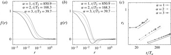
(a) Longitudinal and (b) transverse correlation coefficients. (c) Growth of the integral scale
 $r_{I}$
as a function of
 $t/T_{{\it\alpha}}$
. The circled points correspond to the nondimensional times listed in (a,b). The solid line is
 $r_{I}\propto (t/T_{1})^{0.549}$
, the dotted line is
 $r_{I}\propto (t/T_{2})^{0.92}$
, and the dash-dot line is
 $r_{I}\propto (t/T_{3})^{1.0}$
.

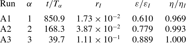
Characteristic times
 $t/T_{{\it\alpha}}$
at which data were taken and corresponding integral scales
 $r_{I}$
, enstrophy flux
 ${\it\eta}$
in the direct cascade and energy flux
 ${\it\varepsilon}$
in the inverse cascade.

The velocity correlation function is
 $$\begin{eqnarray}\mathscr{V}_{ij}(\boldsymbol{r})=\langle v_{i}(\boldsymbol{x})v_{j}(\boldsymbol{x}+\boldsymbol{r})\rangle .\end{eqnarray}$$
Assuming isotropy, so that
 $v^{2}\equiv \langle v_{1}^{2}\rangle =\langle v_{2}^{2}\rangle$
, one can write
 $$\begin{eqnarray}\mathscr{V}_{11}(r\hat{\boldsymbol{e}}_{1})=v^{2}f(r),\quad \mathscr{V}_{22}(r\hat{\boldsymbol{e}}_{1})=v^{2}g(r),\end{eqnarray}$$
where
 $f(r)$
and
 $g(r)$
are the longitudinal and transverse correlation coefficients (Davidson Reference Davidson2004) and
 $\hat{\boldsymbol{e}}_{1}$
is a unit vector lying along the separation direction. The correlation coefficients appear in figure 1(a,b); they remain non-negligible over a larger distance as
 ${\it\alpha}$
increases.
We define the integral scale as
 $$\begin{eqnarray}r_{I}=\sqrt{\frac{\langle {\it\psi}^{2}\rangle }{v^{2}}},\end{eqnarray}$$
where the angle brackets denote an average over the domain (Davidson Reference Davidson2004). The Green’s function (2.3) determines how
 ${\it\theta}$
feeds back on
 ${\it\psi}$
and therefore
 $\boldsymbol{v}$
; this varies with
 ${\it\alpha}$
and will manifest as differences in the growth rate of
 $r_{I}$
. As evident in figure 1(c),
 $r_{I}$
does grow more quickly as
 ${\it\alpha}$
increases, but is still well below the domain scale
 $2{\rm\pi}$
in all three systems at the times given in table 2 (circled points).
In the present simulations the integral scale
 $r_{I}$
follows approximately the same growth law as the inverse energy centroid wavenumber
 $k_{e}^{-1}$
. Identifying
 $k_{e}^{-1}$
with
 $r_{I}$
, we can predict the growth rate of
 $r_{I}$
using an argument after Pouquet et al. (Reference Pouquet, Lesieur, Andre and Basdevant1975), which is presented in appendix A. This yields
 $$\begin{eqnarray}r_{I}\propto t^{{\it\gamma}},\quad {\it\gamma}=1/(n-1),\end{eqnarray}$$
where
 $\mathscr{E}(k)\propto k^{-n}$
for
 $k_{e}<k<k_{f}$
and
 $n$
is assumed to be constant. The latter assumption is justified because the energy spectral exponent
 $n_{av}$
averaged over the range
 $[k_{e},1000]$
varies slowly in our simulations. Using
 $n_{av}$
we computed
 ${\it\gamma}$
for the times shown in figure 1(c) (omitting the first point from the
 ${\it\alpha}=3$
curve) and then time averaged. The time-averaged values were
 $\overline{{\it\gamma}}=0.71\pm 0.03$
for
 ${\it\alpha}=1$
,
 $\overline{{\it\gamma}}=0.92\pm 0.06$
for
 ${\it\alpha}=2$
, and
 $\overline{{\it\gamma}}=1.2\pm 0.1$
for
 ${\it\alpha}=3$
, where the error is the standard deviation. In comparison, the growth laws obtained by fitting lines to the curves in figure 1(c) are
 $r_{I}\propto (t/T_{1})^{0.549\pm 0.009}$
for
 ${\it\alpha}=1$
,
 $r_{I}\propto (t/T_{2})^{0.92\pm 0.06}$
for
 ${\it\alpha}=2$
, and
 $r_{I}\propto (t/T_{3})^{1.0\pm 0.1}$
for
 ${\it\alpha}=3$
. The agreement is very good for
 ${\it\alpha}=2$
and
 ${\it\alpha}=3$
, while for
 ${\it\alpha}=1$
it is not as good. We note that in the latter system much of the energy is found in large vortices, where it may be trapped, slowing the growth of
 $r_{I}$
. Perhaps relatedly, the bulge in
 $\mathscr{E}(k)$
observed at large scales within the inverse cascade disrupts the power law seen closer to the forcing scale, so that the observed spectrum does not take the form
 $\mathscr{E}(k)\propto k^{-n}$
for
 $k_{e}<k<k_{f}$
.
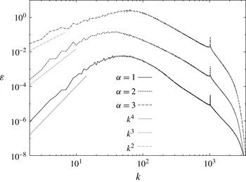
As an additional check that the results do not depend on domain size, we examine the spectral scaling in the low-wavenumber range. Iwayama & Watanabe (Reference Iwayama and Watanabe2014) studied the generalized enstrophy spectrum in this range using a closure for a 2D fluid in an infinite domain and found
 $\mathscr{Z}(k)\propto k^{5}$
as
 $k\rightarrow 0$
. This corresponds to
 $\mathscr{E}(k)\propto k^{5-{\it\alpha}}$
. As shown in figure 2, the systems under study satisfy this relation approximately.
Low-wavenumber scaling of
 $\mathscr{E}(k)$
for
 ${\it\alpha}=1$
at
 $t/T_{1}=850.9$
,
 ${\it\alpha}=2$
at
 $t/T_{2}=168.3$
, and
 ${\it\alpha}=3$
at
 $t/T_{3}=39.7$
. The energy spectra are offset by several decades for clarity. The straight lines correspond to
 $k^{5-{\it\alpha}}$
.

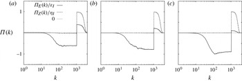
The generalized energy and enstrophy fluxes for the
 $8192^{2}$
simulations appear in figure 3. As evident from the plots, inverse and direct cascades are well developed in all three systems. The fluxes are approximately constant with
 $k$
over substantial spectral ranges, modulo fall-off in the enstrophy cascade due to dissipation. All three systems exhibit downscale as well as upscale energy flux; this is due to the dissipation sink at large
 $k$
, with the inertial range being finite. The downscale energy flux is constant with
 $k$
for a large range of wavenumbers (note the log scale), suggesting that energy is dissipated at scales smaller than the forcing scale. The downscale enstrophy flux is approximately constant with
 $k$
over a similar range. Our results differ from the simulations of Boffetta (Reference Boffetta2007), in which energy that did not cascade upscale was dissipated around the forcing scale, and the downscale enstrophy flux was not constant over any appreciable spectral interval.
Fluxes of generalized energy
 ${\it\Pi}_{E}$
and of generalized enstrophy
 ${\it\Pi}_{Z}$
, normalized by their respective injection rates, for (a)
 ${\it\alpha}=1$
at
 $t/T_{1}=850.9$
, (b)
 ${\it\alpha}=2$
at
 $t/T_{2}=168.3$
, (c)
 ${\it\alpha}=3$
at
 $t/T_{3}=39.7$
. Positive values indicate downscale fluxes, and negative values upscale fluxes. These fluxes correspond to the spectra in figure 4.

The downscale energy flux
 ${\it\Pi}_{E}^{dir}=k_{d}^{-{\it\alpha}}{\it\Pi}_{Z}^{dir}\leqslant k_{d}^{-{\it\alpha}}{\it\eta}_{I}=(k_{f}/k_{d})^{{\it\alpha}}$
, since
 ${\it\eta}_{I}=k_{f}^{{\it\alpha}}{\it\varepsilon}_{I}$
and
 ${\it\varepsilon}_{I}=1$
, so
 ${\it\Pi}_{E}^{dir}/{\it\varepsilon}_{I}$
decreases as
 ${\it\alpha}$
increases. This is reflected in table 2: 61.0 % of the injected generalized energy cascades upscale for
 ${\it\alpha}=1$
, while for
 ${\it\alpha}=2$
the percentage is 77.9 %, and for
 ${\it\alpha}=3$
it is 88.9 %.
5. Coherent structures and spectral steepening
5.1. Total energy spectra
Generalized energy spectra for the three systems under study appear in figure 4. We average over eleven consecutive diagnostic time steps to reduce noise; this does not appreciably affect the measured slopes. The averaging extends from
 $t/T_{1}=763.4$
to
 $t/T_{1}=850.9$
,
 $t/T_{2}=121.5$
to
 $t/T_{2}=215.0$
, and
 $t/T_{3}=34.9$
to
 $t/T_{3}=44.6$
, where
 $T_{{\it\alpha}}$
is the time scale defined in (4.2). We must take data from earlier nondimensional times at larger
 ${\it\alpha}$
due to the faster growth of
 $r_{I}$
discussed above – see figure 1(c). A spike centred on
 $k_{f}=1024$
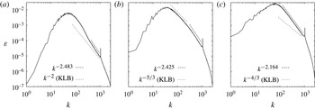
marks the forcing band, and inverse- and direct-cascading inertial ranges are identifiable in each plot.
Inverse cascade energy spectra for (a)
 ${\it\alpha}=1$
, (b)
 ${\it\alpha}=2$
and (c)
 ${\it\alpha}=3$
averaged over times
 $t/T_{1}=763.4{-}850.9$
,
 $t/T_{2}=121.5{-}215.0$
and
 $t/T_{3}=34.9{-}44.6$
respectively, together with best fit and KLB power laws indicated by straight lines. Part of the direct cascade range is also shown.

In all three systems, the inverse cascade spectral slope is steeper than the KLB prediction. The dash-dot lines represent linear fits, while the dashed lines represent the KLB scaling. For
 ${\it\alpha}=1$
we observe a well-defined power law with slope
 $-2.483\pm 0.003$
in the range
 $k\approx 300$
to
 $k\approx 900$
, where the uncertainty is the standard error. This is steeper than the KLB slope
 $-2$
. At
 $k<300$
the spectrum becomes rounded and the power law scaling is lost, as evident in figure 4(a).
For
 ${\it\alpha}=2$
the inverse cascade spectrum does not follow a single clear power law scaling, consistent with the findings of Danilov & Gurarie (Reference Danilov and Gurarie2001), who argued that the ‘ideal cascade state’ was not achievable, and one would have either a spectral bulge or flux distortion. The shape suggests a two-part spectrum steeper than the KLB scaling
 $-5/3$
at higher
 $k$
, where the slope is
 $-2.425\pm 0.004$
over the range
 $k=300$
to
 $k=850$
, and close to the KLB scaling at lower
 $k$
, where the slope is
 $-1.683\pm 0.009$
over the range
 $k=52$
to
 $k=250$
.
For
 ${\it\alpha}=3$
we observe
 $-2.164\pm 0.002$
in the simulated inverse cascade, again steeper than the KLB prediction
 $-4/3$
. The power law is the cleanest of the three systems, and the slope is close to the absolute equilibrium slope
 $-2$
associated with equipartition of generalized enstrophy for
 ${\it\alpha}=3$
(Burgess & Shepherd Reference Burgess and Shepherd2013). In such an equipartition state the statistics are Gaussian and, since the system is in equilibrium, the transfers vanish. Although the transfers do not vanish here, since this would be at odds with a turbulent cascade, which we clearly observe, we will find that the statistics are the closest to Gaussian of the three systems under study. This suggests that the inverse cascade for
 ${\it\alpha}=3$
is in a state close to equipartition of generalized enstrophy.
It is important to emphasize that the inverse cascade has not reached the domain scale in any of the systems. Moreover, the slopes do not depend strongly on how developed the inverse cascade is – they are steeper than the KLB spectra and close to those given in figure 4 at much earlier stages of the simulation. This is further confirmation that the steep spectra observed are not due to condensation into the lowest mode.
5.2. Active scalar and velocity fields
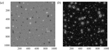
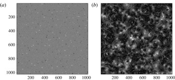
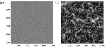
Snapshots of the active scalar (
 ${\it\theta}$
) fields appear in the panels (a) of figures 5–7. Conspicuous coherent vortices are visible in the flow for
 ${\it\alpha}=1$
and
 ${\it\alpha}=2$
. For
 ${\it\alpha}=3$
small axisymmetric vortices appear but do not persist – they are stretched out and destroyed by the ambient shear. For both
 ${\it\alpha}=1$
and
 ${\it\alpha}=2$
a range of vortex sizes and strengths are present, but the vortices span a broader range of sizes for
 ${\it\alpha}=1$
than for
 ${\it\alpha}=2$
. Merger occurs in both systems – two negative vortices appear to be merging at (
 ${\sim}250,\sim 125$
) in figure 5(a). Two negative
 ${\it\alpha}=2$
vortices are in close proximity and appear to be merging at (
 ${\sim}150,\sim 650$
) in figure 6(a), and two positive vortices in similar close approach are also visible at (
 ${\sim}500,\sim 425$
). The characteristic scale of the active scalar field grows visibly smaller as
 ${\it\alpha}$
increases, which is consistent with a larger-scale separation between streamfunction (or velocity) and generalized vorticity. For
 ${\it\alpha}=3$
vortices are short-lived and seem to exist near the edges of high-velocity regions, where the shear is perhaps weakest.
(a)
 $~{\it\theta}$
and (b)
 $|\boldsymbol{v}|$
for
 ${\it\alpha}=1$
in a
 $1024^{2}$
region at
 $t/T_{1}=850.9$
. The axes are labelled with the distance in grid sites.

(a)
 ${\it\theta}$
and (b)
 $|\boldsymbol{v}|$
for
 ${\it\alpha}=2$
in a
 $1024^{2}$
region at
 $t/T_{2}=168.3$
. The axes are labelled with the distance in grid sites.

(a)
 ${\it\theta}$
and (b)
 $|\boldsymbol{v}|$
for
 ${\it\alpha}=3$
in a
 $1024^{2}$
region at
 $t/T_{3}=39.7$
. The axes are labelled with the distance in grid sites.

The panels (b) of figures 5–7 show the speed fields corresponding to the active scalar fields in corresponding panels (a). For
 ${\it\alpha}=1$
the high-velocity structures are strikingly circular, have well-defined edges, and centre on vortex cores, which appear as low-velocity punctures in the flow. Regions of high velocity also surround vortex cores for
 ${\it\alpha}=2$
, but their edges are not as well defined and they reflect the filamentary structure of the vorticity field. The velocity field becomes more filamentary as
 ${\it\alpha}$
increases, and is dominated by sinuous high-speed regions for
 ${\it\alpha}=3$
, which are comparatively structurally unrelated to the small vortices in the flow. This is again consistent with the increasing scale separation between the streamfunction
 ${\it\psi}$
and advected scalar
 ${\it\theta}$
as
 ${\it\alpha}$
increases. For
 ${\it\alpha}=1$
the velocity field is clearly organized around axisymmetric vortices, but this becomes less true as
 ${\it\alpha}$
increases.
It is interesting to note that the existence of coherent vortices does not appear to be related to the large-scale spectra. As discussed above,
 $\mathscr{E}(k)\sim k^{5-{\it\alpha}}$
at the largest scales, indicating greater spectral nonlocality at larger
 ${\it\alpha}$
. In contrast, figures 5–7 clearly show a reduction in the dominance of coherent vortices with increasing
 ${\it\alpha}$
.
5.3. Interstitial spectrum from continuous wavelet analysis
We use continuous wavelet analysis to study the comparatively weak interstitial field surrounding the high-amplitude vortices. In contrast to the spatially delocalized sinusoids of Fourier analysis, wavelets are local in both space and scale, which is advantageous when – as here – the field is spatially inhomogeneous and its spectral content will differ from one location to another. The continuous wavelet transform of a 2D field
 $f(\boldsymbol{x})$
is
 $$\begin{eqnarray}\tilde{f}(r,\boldsymbol{x}^{\prime },{\it\phi})=\int _{-\infty }^{\infty }\int _{-\infty }^{\infty }f(\boldsymbol{x}){\it\Psi}_{r,\boldsymbol{x}^{\prime },{\it\phi}}^{\ast }(\boldsymbol{x})\text{d}^{2}\boldsymbol{x},\end{eqnarray}$$
where the ‘daughter’ wavelet
 $$\begin{eqnarray}{\it\Psi}_{r,\boldsymbol{x}^{\prime },{\it\phi}}(\boldsymbol{x})=r^{-1}{\it\Psi}\left[R_{{\it\phi}}^{-1}\left(\frac{\boldsymbol{x}-\boldsymbol{x}^{\prime }}{r}\right)\right]\end{eqnarray}$$
is a rotated, translated and dilated version of a ‘mother wavelet’. To be a wavelet, a function
 ${\it\Psi}(\boldsymbol{x})\in L^{2}(\mathbb{R}^{2})$
must satisfy the ‘admissibility condition’,
 $$\begin{eqnarray}C_{{\it\Psi}}=\int _{-\infty }^{\infty }\int _{-\infty }^{\infty }|\hat{{\it\Psi}}(\boldsymbol{k})|^{2}k^{-2}\text{d}^{2}\boldsymbol{k}<\infty ,\end{eqnarray}$$
where
 $\hat{{\it\Psi}}(\boldsymbol{k})$
is the Fourier transform. If
 ${\it\Psi}$
is integrable, then (5.3) implies
 $\hat{{\it\Psi}}(0)=0$
, i.e. that
 ${\it\Psi}$
has zero mean. Anisotropic wavelets carry the index
 ${\it\phi}$
, which specifies the analysis direction. The dilation parameter
 $r>0$
and translation vector
 $\boldsymbol{x}^{\prime }$
vary continuously, and the wavelets form an overcomplete basis, but can provide information at any desired scale and location. It is also possible to construct orthonormal discrete wavelet bases, in which the translations and dilations take values on a dyadic grid; these form an orthonormal basis for
 $L^{2}(\mathbb{R}^{2})$
and are used for multiresolution analysis (Daubechies Reference Daubechies1992), but offer much less scale selectivity than does the continuous wavelet transform. Further details on wavelets can be found in Daubechies (Reference Daubechies1992). Farge et al. (Reference Farge, Guezennec, Ho and Meneveau1990) used the continuous wavelet transform to study turbulence, while Kevlahan & Farge (Reference Kevlahan and Farge1997), Farge, Schneider & Kevlahan (Reference Farge, Schneider and Kevlahan1999) and Beta, Schneider & Farge (Reference Beta, Schneider and Farge2004) used orthonormal wavelets to extract vortices from 2D turbulence (
 ${\it\alpha}=2$
) and define coherent and incoherent fields.
For our analysis we used the Fan wavelet, constructed by averaging a series of 2D Morlet wavelets over a finite number of directions, and which reproduces a power law Fourier spectrum closely when the spectrogram is summed over
 $\boldsymbol{x}^{\prime }$
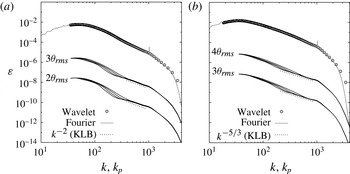
(Kirby Reference Kirby2005). The globally averaged wavelet spectrogram (black circles) appears in figure 8 plotted against an equivalent Fourier wavenumber
 $k_{p}$
(the wavenumber at which the daughter wavelet reaches its maximum value). As is evident the wavelet spectrogram reproduces the Fourier spectrum (solid grey line) very well, departing only at the highest wavenumbers.
To qualify as ‘interstitial’ we required the field at a given location
 $\boldsymbol{x}$
to satisfy
 ${\it\theta}(\boldsymbol{x})<{\it\theta}_{thr}$
, and we also required
 ${\it\theta}(\boldsymbol{x}+\boldsymbol{x}^{\prime })<{\it\theta}_{thr},|\boldsymbol{x}^{\prime }|\leqslant i_{dx}{\rm\Delta}x$
, where
 ${\rm\Delta}x$
is the grid spacing and
 $i_{dx}$
a specified number of grid sites. We performed a sensitivity study, taking
 $i_{dx}=\{10,20,30,40\}$
and choosing
 ${\it\theta}_{thr}=\{2{\it\theta}_{rms},3{\it\theta}_{rms}\}$
for
 ${\it\alpha}=1$
and
 ${\it\theta}_{thr}=\{3{\it\theta}_{rms},4{\it\theta}_{rms}\}$
for
 ${\it\alpha}=2$
. These values of
 ${\it\theta}_{thr}$
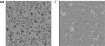
represent reasonable choices in that they exclude most of the concentrated axisymmetric vorticity structures from the interstitial field. Sample interstitial fields are shown in figure 9 for
 ${\it\alpha}=1$
with
 ${\it\theta}_{thr}=3{\it\theta}_{rms}$
and
 $i_{dx}=20$
(a) and
 ${\it\alpha}=2$
with
 ${\it\theta}_{thr}=4{\it\theta}_{rms}$
and
 $i_{dx}=40$
(b). The wavelet spectrograms averaged over the interstitial fields are plotted as solid black lines in figure 8, with the KLB scaling (dashed line) for comparison. In both systems, for both choices of
 ${\it\theta}_{thr}$
, an interstitial spectrum with approximate KLB scaling appears above the forcing scale. For
 ${\it\alpha}=1$
this KLB range is clearly present even for
 $i_{dx}=10$
, while for
 ${\it\alpha}=2$
the KLB range extends as
 $i_{dx}$
increases from 10 to 40, consistent with the longer-range effect of the vortices in the latter system. The spectral slope is more sensitive to
 ${\it\theta}_{thr}$
for
 ${\it\alpha}=1$
than for
 ${\it\alpha}=2$
, falling somewhat below the KLB value
 $-2$
for
 ${\it\theta}_{thr}=2{\it\theta}_{rms}$
. For
 ${\it\alpha}=2$
both choices of
 ${\it\theta}_{thr}$
yield clean KLB scaling ranges. The results of the wavelet analysis thus show that the weak interstitial flows in both systems exhibit the KLB spectrum, though the slope is more sensitive to
 ${\it\theta}_{thr}$
for
 ${\it\alpha}=1$
than for
 ${\it\alpha}=2$
.
Wavelet and Fourier spectra for (a)
 ${\it\alpha}=1$
and (b)
 ${\it\alpha}=2$
. The Fourier spectrum (grey) is overlain on the globally averaged wavelet spectrogram (black circles). Wavelet spectrograms for the interstitial flow (solid black lines) with two choices of
 ${\it\theta}_{thr}$
and
 $i_{dx}=10,20,30$
and 40 (from top to bottom) also appear, together with KLB scaling (dashed black lines).

Sample interstitial flow (light regions) for (a)
 ${\it\alpha}=1$
(
 ${\it\theta}_{thr}=3{\it\theta}_{rms}$
,
 $i_{dx}=20$
) and (b)
 ${\it\alpha}=2$
(
 ${\it\theta}_{thr}=4{\it\theta}_{rms}$
,
 $i_{dx}=40$
).

6. Measures of Gaussianity and intermittency
We calculate several measures of Gaussianity and intermittency for the simulated flows, our focus being the impact of
 ${\it\alpha}$
on these properties. We also calculate velocity structure functions for the interstitial
 ${\it\alpha}=1$
and
 ${\it\alpha}=2$
fields to further probe whether these fields satisfy the assumptions of classical KLB phenomenology. We begin with one- and two-point active scalar p.d.f.s, followed by hyperflatness factors and structure functions.
6.1. Active scalar and velocity probability density functions
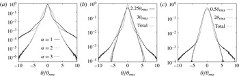
The one-point probability density functions of the total active scalar fields appear in figure 10(a). The p.d.f.s are averaged over eleven consecutive time steps for
 ${\it\alpha}=1,2$
, while for
 ${\it\alpha}=3$
we take a longer averaging period of twenty-one time steps because the p.d.f. is noisier. We calculate kurtosis directly from the fields and average over the same time steps to obtain
 $K_{{\it\theta}}$
.
(a) Averaged one-point active scalar p.d.f.s. The corresponding averaged kurtoses are
 $K_{{\it\theta}}=22.99,22.09,3.97$
for
 ${\it\alpha}=1,2,3$
respectively. (b,c) Total and filtered one-point active scalar p.d.f.s for
 ${\it\alpha}=1$
and
 ${\it\alpha}=2$
respectively. The values of
 ${\it\theta}_{thr}$
used for filtering are given at the top right.

For
 ${\it\alpha}=1$
and
 ${\it\alpha}=2$
the p.d.f.s have broad and visibly non-Gaussian tails. The averaged kurtoses for
 ${\it\alpha}=1$
and
 ${\it\alpha}=2$
are
 $K_{{\it\theta}}=22.99$
and
 $K_{{\it\theta}}=22.09$
respectively, over seven times the Gaussian value
 $K_{{\it\theta}}=3$
. Kurtosis is a measure of spatial intermittency in the sense that if the vorticity field is concentrated on squares of side length
 $a$
separated by distance
 $b$
, then
 $K\propto (b/a)^{2}$
(McWilliams Reference McWilliams1984). The high values of kurtosis found here for
 ${\it\alpha}=1$
and
 ${\it\alpha}=2$
reflect the spatial intermittency associated with the intense vortices in these flows. Maltrud & Vallis (Reference Maltrud and Vallis1991) obtained much lower values for the vorticity kurtosis in the
 ${\it\alpha}=2$
cascade, at
 $K_{{\it\theta}}\approx 3.5{-}4$
. However, their simulations were forced near the highest resolved wavenumber and utilized large-scale drag. Paret & Tabeling (Reference Paret and Tabeling1998) obtained
 $K_{{\it\theta}}\approx 5$
for
 ${\it\alpha}=2$
. For
 ${\it\alpha}=3$
the one-point p.d.f. appears closer to Gaussian and has a much lower averaged kurtosis, at
 $K_{{\it\theta}}=3.97$
, which is notably still non-Gaussian. This comparatively low level of non-Gaussianity is consistent with the close-to-equipartition spectrum in this model’s inverse-cascading inertial range.
To examine further the role of coherent vortices in the one-point p.d.f. shapes, particularly the ‘double-shouldered’ p.d.f. for
 ${\it\alpha}=1$
, we compute the same quantities for residual fields obtained by removing the vortices with a simple thresholding and smoothing procedure (see appendix B). We expect this procedure to yield reasonably reliable information about the one-point statistics because they are not sensitive to gradients. The total
 ${\it\alpha}=1$
p.d.f. has an undulation between
 ${\it\theta}/{\it\theta}_{rms}\approx 2.5$
and
 ${\it\theta}/{\it\theta}_{rms}\approx 6$
, which appears to be associated with the broad ‘skirts’ of the highly strained
 ${\it\theta}$
field surrounding the cores of the
 ${\it\alpha}=1$
vortices as seen in figure 5. As is evident from comparing the one-point p.d.f.s obtained from the residual fields with
 ${\it\theta}_{thr}=2.25{\it\theta}_{rms}$
and
 ${\it\theta}_{thr}=3{\it\theta}_{rms}$
in figure 10(b), the undulation develops as
 ${\it\theta}_{thr}$
increases, including more of the skirt in the residual field.
The residual one-point p.d.f.s for
 ${\it\alpha}=2$
in figure 10(c) are close to Gaussian and the results for the two values of
 ${\it\theta}_{thr}$
are visually indistinguishable. They lack the broad tails of the total one-point p.d.f., demonstrating that these tails are associated with the coherent vortices. This result is not surprising, since removing extreme events will remove broad tails, and is consistent with the wavelet decompositions performed by Farge et al. (Reference Farge, Schneider and Kevlahan1999) and Beta et al. (Reference Beta, Schneider and Farge2004), the latter of which showed that the non-Gaussian part of the vorticity field in
 ${\it\alpha}=2$
turbulence forced at
 $k_{f}=4$
corresponded to coherent vortices.
We also compute one-point active scalar p.d.f.s for the field smoothed at length scale
 $l$
,
 $$\begin{eqnarray}\overline{{\it\theta}}_{l}(\boldsymbol{x})=\int \text{d}\boldsymbol{r}~G_{l}(\boldsymbol{r}){\it\theta}(\boldsymbol{x}+\boldsymbol{r}),\end{eqnarray}$$
where
 $G_{l}(\boldsymbol{r})=l^{-2}G(\boldsymbol{r}/l)$
and
 $G(\boldsymbol{r})$
is any smooth, rapidly decaying positive function with unit integral (Germano Reference Germano1992). We choose a 2D Gaussian smoothing kernel,
 $$\begin{eqnarray}G_{l}(\boldsymbol{r})=\frac{1}{2{\rm\pi}{\it\sigma}^{2}}\exp \left[-\frac{1}{2{\it\sigma}^{2}}\left(\frac{r}{l}\right)^{2}\right],\end{eqnarray}$$
with
 ${\it\sigma}=\sqrt{2}$
, and filter by convolution with the kernel in Fourier space. The field
 $\overline{{\it\theta}}_{l}(\boldsymbol{x})$
can be interpreted as
 ${\it\theta}$
averaged over fluid parcels of size
 $l$
centred at
 $\boldsymbol{x}$
.
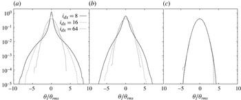
The one-point p.d.f.s of
 $\overline{{\it\theta}}_{l}$
with
 $l=i_{dx}{\rm\Delta}x$
appear in figure 11. Smoothing at
 $i_{dx}=8$
corresponds to smoothing at the forcing scale,
 $k_{f}=1024$
, while
 $i_{dx}=16$
and
 $i_{dx}=64$
correspond to
 $k=512$
and
 $k=128$
respectively. Increasing the smoothing scale progressively removes the broad tails and restores a Gaussian shape to the
 ${\it\alpha}=1,2$
p.d.f.s, while it hardly affects the
 ${\it\alpha}=3$
p.d.f. at all. The one-point
 ${\it\theta}$
statistics for
 ${\it\alpha}=3$
thus appear the same when coarse-grained at and above
 $k_{f}=1024$
, while for
 ${\it\alpha}=1,2$
this is not true. This presumably reflects the presence of vortices at and above the forcing scale for
 ${\it\alpha}=1,2$
, while for
 ${\it\alpha}=3$
the p.d.f. is already close to Gaussian and so does not change appreciably in response to smoothing.
Smoothed one-point active scalar p.d.f.s for (a)
 ${\it\alpha}=1$
, (b)
 ${\it\alpha}=2$
,and (c)
 ${\it\alpha}=3$
.

Schorghofer (Reference Schorghofer2000) found universality of the one-point p.d.f.s of
 ${\it\theta}$
,
 $\partial _{x}{\it\theta}$
, scalar dissipation
 $D|\boldsymbol{{\rm\nabla}}{\it\theta}|^{2}$
and
 $v_{x}$
in the direct cascades for
 ${\it\alpha}=1,2,3$
. In contrast, the one-point active scalar p.d.f.s in figures 10 and 11 show that, at least in the inverse cascade, certain one-point statistics depend on the effective nonlinearity in the advection term as controlled by
 ${\it\alpha}$
. Total two-point p.d.f.s normalized by
 $\sqrt{S_{2}}$
appear in figure 12. In all three systems the active scalar p.d.f.s (a,d,g) have a Gaussian central peak and broad tails consistent with the presence of vortices. As
 ${\it\alpha}$
increases from 1 to 3 it is as though one ‘zooms in’ on the Gaussian central peak, which occupies more and more of the distribution, consistent with the decreasing number and size of vortices as
 ${\it\alpha}$
increases. For
 ${\it\alpha}=2$
the tails are broader for separations lying at inverse cascade scales. For
 ${\it\alpha}=1$
there are again two undulations in the inverse cascade p.d.f.s associated with the ‘two-part’ vortex profile consisting of a Gaussian peak and a broad skirt; in contrast the
 ${\it\alpha}=2$
and
 ${\it\alpha}=3$
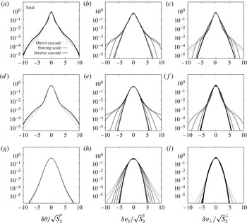
p.d.f.s have only one undulation and the tails fan out more sharply, reflecting the fact that vortices in these systems do not have skirts, at least at the stage of evolution considered. There is little intermittency evident in the two-point active scalar plots, especially for separations in the inverse cascade, as the p.d.f.s have approximately the same shape regardless of separation distance.
Two-point p.d.f.s for (a–c)
 ${\it\alpha}=1$
, (d–f)
 ${\it\alpha}=2$
and (g–i)
 ${\it\alpha}=3$
. (a,d,g) p.d.f.s of active scalar increments, (b,e,h) longitudinal velocity increments and (c,f,i) transverse velocity increments. The separations considered correspond to
 $2^{m}k_{f}$
, where
 $m=2,1,0,-1,-2,-3,-4,-5,-6,-7,-8,-9$
.

The longitudinal velocity-increment p.d.f.s (figure 12 b,e,h) also have broad tails for some separations. The most striking difference as compared to the active scalar-increment p.d.f.s is the scale-dependence of the p.d.f. shapes: they become more Gaussian as the scale increases and are much more Gaussian at the largest scales of the inverse cascade than in the direct cascade. In contrast, the p.d.f.s for separations lying in the direct cascade range all have similar shapes, though again with broad tails.
Especially for
 ${\it\alpha}=1$
and
 ${\it\alpha}=2$
the transverse velocity-increment p.d.f.s (figure 12
c,f,i) are also scale-dependent. Again, the p.d.f.s have broad tails in the direct cascade and recover a more Gaussian shape at inverse cascade scales. Our results are consistent with previous studies on
 ${\it\alpha}=2$
that found approximately Gaussian statistics for the inverse cascade velocity differences (Paret & Tabeling Reference Paret and Tabeling1998). Of the models studied here,
 ${\it\alpha}=3$
has transverse velocity-increment p.d.f.s closest to Gaussian; they are notably more Gaussian and non-intermittent than the p.d.f.s of longitudinal velocity increments.
The scale-dependence of the velocity-increment p.d.f. shapes indicates that the quasi-steady inverse cascades we simulate here are intermittent, i.e. there is scale-dependence of the statistics of velocity increments at least over a portion of the inverse cascade in these simulations. The spectral range over which the p.d.f.s change shape is approximately
 $k_{f}$
to
 $k_{f}/8$
, with some variation depending on
 ${\it\alpha}$
and on whether the increments are longitudinal or transverse. This spectral range includes the vortex-containing scales where the interstitial field exhibits KLB scaling and the range where the total
 ${\it\alpha}=1$
spectrum follows a power law.
In summary, the p.d.f.s of active scalar increments are non-Gaussian and non-intermittent in all three systems, though those of
 ${\it\alpha}=3$
are the closest to Gaussian. Their broad tails are associated with vortices, as confirmed by comparing with the p.d.f.s for the interstitial fields (not shown). In contrast, the velocity-increment p.d.f.s generally have broad tails, but recover a more Gaussian shape at the largest scales in the inverse cascade. This is true of all three models, but again
 ${\it\alpha}=3$
is the closest to Gaussian. The velocity p.d.f.s of the interstitial fields (not shown) are less intermittent, demonstrating that scale dependence is due to vortices. The inverse cascades in these simulations thus appear to be intermittent and to recover Gaussianity at the largest scales, at least as reflected in the velocity field. At the largest scales the inverse cascades are much more Gaussian than the direct cascades, consistent with previous results for
 ${\it\alpha}=2$
(Paret & Tabeling Reference Paret and Tabeling1998).
6.2. Hyperflatness factors
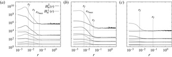
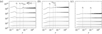
The hyperflatness factors of the velocity and active scalar increments, which appear in figures 13 and 14, are an alternative presentation of the statistics encoded in the two-point p.d.f.s of § 6.1. The forcing scale
 $r_{f}$
, size of the largest vortex
 $r_{V_{max}}$
(for
 ${\it\alpha}=1$
and
 ${\it\alpha}=2$
), and the integral scale
 $r_{I}$
are marked on the plots. Interestingly,
 $r_{I}$
falls below
 $r_{V_{max}}$
for
 ${\it\alpha}=1$
. The departure of the inverse cascade velocity hyperflatness factors from Gaussianity decreases as
 ${\it\alpha}$
increases, consistent with the p.d.f. shapes. The velocity hyperflatness factors stabilize farthest above the Gaussian values for
 ${\it\alpha}=1$
, perhaps reflecting the prominent role of large vortices in the flow. In all three systems the transverse velocity hyperflatness factors depart more from Gaussianity than do the longitudinal hyperflatness factors in the direct cascade, while they lie on top of each other – modulo noise – in the inverse cascade.
Hyperflatness factors of longitudinal and transverse velocity increments for (a)
 ${\it\alpha}=1$
, (b)
 ${\it\alpha}=2$
and (c)
 ${\it\alpha}=3$
. The straight horizontal lines are the Gaussian values. The vertical lines mark the forcing scale
 $r_{f}$
, the integral scale
 $r_{I}$
and the maximum vortex diameter
 $r_{V_{max}}$
, where applicable. The ranges on the vertical axes are the same in each panel to facilitate comparison.

Hyperflatness factors of active scalar increments for (a)
 ${\it\alpha}=1$
, (b)
 ${\it\alpha}=2$
and (c)
 ${\it\alpha}=3$
. The straight horizontal lines are the Gaussian values. The vertical lines mark the forcing scale
 $r_{f}$
, the integral scale
 $r_{I}$
and the maximum vortex diameter
 $r_{V_{max}}$
, where applicable. The ranges on the vertical axes are the same in each panel to facilitate comparison.

The stabilization of the velocity hyperflatness factors at constant values with separation in the inverse cascade is another indication that the statistics are not scale-dependent at large scales. The hyperflatness factors decrease through the vortex-containing scales for both
 ${\it\alpha}=1$
and
 ${\it\alpha}=2$
. For
 ${\it\alpha}=1$
the levelling of the velocity hyperflatness factors coincides with
 $r_{V_{max}}$
, while for
 ${\it\alpha}=2$
they continue to decrease above
 $r_{V_{max}}$
; this probably reflects the fact that the velocity and active scalar fields are of the same scale for
 ${\it\alpha}=1$
, while for
 ${\it\alpha}=2$
the vorticity field is of a smaller scale than the velocity field. Comparing figure 13(a) and (b) one sees that
 $r_{V_{max}}$
and
 $r_{I}$
seem to be good measures of the saturation/decorrelation length for
 ${\it\alpha}=1$
and
 ${\it\alpha}=2$
respectively.
The active scalar hyperflatness factors are above the non-Gaussian values in all three systems. This is consistent with figure 12(a,d,g), which shows that the corresponding p.d.f.s have broader tails in the inverse cascade than do the velocity-increment p.d.f.s shown in the figure 12(b,e,h) and (c,f,i), the tails of which narrow towards a Gaussian shape at increasing separations. The
 ${\it\alpha}=3$
active scalar hyperflatness factors are less non-Gaussian then those of the other two systems, which are comparable to each other. The active scalar increments are non-intermittent, as evidenced by the constancy of the hyperflatness factors with separation distance, as well as the relative scale invariance of the p.d.f. shapes in figure 12(a,d,g).
6.3. Structure functions
As a second test for intermittency, we compute structure function scaling exponents in the inverse cascades for ranges where scaling is well defined. We use ESS, plotting versus third-order structure functions, for more accurate detection of scaling ranges (Benzi et al. Reference Benzi, Ciliberto, Tripiccione, Baudet, Massaioli and Succi1993).
To check the convergence of the high-order moments, we used the method suggested by Paret & Tabeling (Reference Paret and Tabeling1998), namely studying the smoothness and monotonicity of the curves
 $|{\it\delta}v|^{n}p_{r}^{\Vert }({\it\delta}v)$
,
 $|{\it\delta}v|^{n}p_{r}^{\bot }({\it\delta}v)$
and
 $|{\it\delta}{\it\theta}|^{n}p_{r}({\it\delta}{\it\theta})$
, where
 $p_{r}^{\Vert }({\it\delta}v)$
and
 $p_{r}^{\bot }({\it\delta}v)$
are the probabilities of measuring, over a separation
 $r$
, longitudinal and transverse velocity increments
 ${\it\delta}v$
, and
 $p_{r}({\it\delta}{\it\theta})$
is the probability of measuring an active scalar increment
 ${\it\delta}{\it\theta}$
. As the order
 $n$
increases, these curves are increasingly sensitive to the tails of the p.d.f.; the poorer the convergence, the noisier the curves, as exhibited by large fluctuations and attendant non-monotonic decrease to zero at large
 $|v|$
and
 $|{\it\theta}|$
. We found that the higher-order velocity moment curves (not shown) were remarkably smooth for separations in the inverse cascade and had well-defined shapes decreasing to zero. The smoothness was greatest for
 ${\it\alpha}=3$
, for which the curves decreased to zero monotonically even at order
 $n=12$
. This suggests the high-order velocity moments are reasonably well converged. In contrast, the high-order
 ${\it\theta}$
moments were very noisy for
 ${\it\alpha}=3$
, but are also saturated.
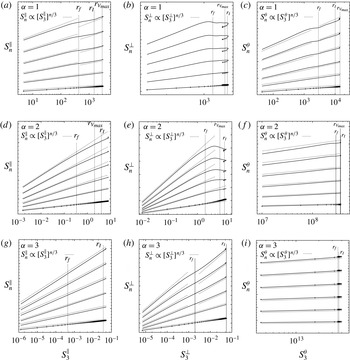
The longitudinal structure functions appear in figure 15(a,d,g). They are scaled by constant multiplicative factors (not shown) where necessary to separate the curves, since we are interested in the shapes and logarithmic slopes of the structure functions and not their magnitudes. The structure functions plotted as functions of
 $S_{3}^{\Vert }(r)$
exhibit clear scaling ranges. At large
 $S_{3}^{\Vert }(r)$
, which corresponds to large scales, the points tend to cluster together – this is a manifestation of the structure functions saturating at large scales (as do the hyperflatness factors in figures 13 and 14).
Structure functions for (a–c)
 ${\it\alpha}=1$
, (d–f)
 ${\it\alpha}=2$
and (g–i)
 ${\it\alpha}=3$
for even orders from
 $n=2$
(lowest curve in each plot) to
 $n=12$
(top curve in each plot). (a,d,g) longitudinal velocity, (b,e,h) transverse velocity and (c,f,i) active scalar structure functions. Straight lines with the scaling
 $n/3$
are plotted for comparison. The forcing scale
 $r_{f}$
, maximum vortex size
 $r_{V_{max}}$
, and integral scale
 $r_{I}$
are marked by vertical dashed lines.

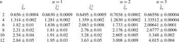
The values of the logarithmic slopes for the longitudinal structure functions appear in table 3; they were calculated using a linear regression model applied to appropriate intervals above the forcing scale
 $r_{f}$
. As is evident in figure 15(a), for
 ${\it\alpha}=1$
the longitudinal velocity structure functions appear to recover the scaling
 $S_{n}^{\Vert }(r)\propto [S_{3}^{\Vert }]^{n/3}$
at large scales, so we split the inverse cascade into two intervals, corresponding to
 $r\in [0.007,0.021]$
and
 $r\in [0.021,0.067]$
, and computed scaling exponents
 $\tilde{{\it\zeta}}_{n}^{1}$
and
 $\tilde{{\it\zeta}}_{n}^{2}$
over each interval as well as the entire range. The fit ranges were chosen based on visual estimation of the scaling ranges. The exponents are indeed closer to
 $n/3$
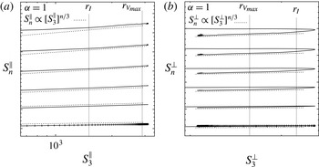
in the larger-scale range. Figure 16(a) shows the large-scale behaviour of the longitudinal structure functions, which recover the
 $n/3$
scaling at and above
 ${\sim}r_{I}$
.
(a) Longitudinal and (b) transverse velocity structure functions for
 ${\it\alpha}=1$
at large scales for even orders from
 $n=2$
(lowest curve in each plot) to
 $n=12$
(top curve in each plot). The point density is shown on the bottom curve. Straight lines with the scaling
 $n/3$
are plotted for comparison. The maximum vortex size
 $r_{V_{max}}$
and integral scale
 $r_{I}$
are marked by vertical dashed lines.

Relative scaling exponents
 $\tilde{{\it\zeta}}_{n}$
of longitudinal velocity structure functions at inverse cascade scales for
 ${\it\alpha}=1$
,
 ${\it\alpha}=2$
and
 ${\it\alpha}=3$
for even orders from
 $n=2$
(lowest curve) to
 $n=12$
(top curve). The latter are closest to
 $n/3$
. For
 ${\it\alpha}=1$
,
 $\tilde{{\it\zeta}}_{n}^{1}$
and
 $\tilde{{\it\zeta}}_{n}^{2}$
are the scaling exponents on the smaller- and larger-scale ranges of the inverse cascade, as discussed in the text.

For
 ${\it\alpha}=2$
we separately computed the exponents in the intervals
 $(r_{f},r_{V_{max}})$
and
 $(r_{V_{max}},r_{I})$
. The exponents were larger in the interval
 $(r_{f},r_{V_{max}})$
. The overall values
 $\tilde{{\it\zeta}}_{n}$
shown in table 3 are dominated by the slope at
 $r>r_{V_{max}}$
because most of the points are located on this interval. The degree of intermittency in the inverse cascade indicated by the structure functions decreases as
 ${\it\alpha}$
increases: the
 ${\it\alpha}=3$
longitudinal structure functions are closest to the scaling
 $n/3$
at all orders, as is evident from figure 15(g) and the right column of table 3.
For
 ${\it\alpha}=1$
and
 ${\it\alpha}=2$
the transverse velocity structure functions shown in figure 15(b,e,f) turn over at inverse cascade scales, while for
 ${\it\alpha}=3$
they exhibit clean scaling. Approximate
 $n/3$
scaling reappears at large scales, so the
 ${\it\alpha}=3$
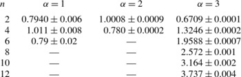
inverse cascade is also non-intermittent as measured by the transverse velocity structure functions at sufficiently large scales. The scaling exponents appear in table 4. At scales larger than
 $r_{I}$
, a very clean
 $n/3$
scaling range emerges for
 ${\it\alpha}=1$
in the transverse velocity structure functions (figure 16
b), indicating non-intermittency of these statistics at these scales.
Relative scaling exponents
 $\tilde{{\it\zeta}}_{n}$
of transverse velocity structure functions.

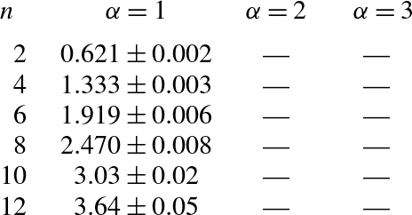
Lastly, active scalar structure functions appear in figure 15(c,f,i) and their measured scaling exponents in table 5. As evident, saturation at large scales is even more pronounced in the active scalar structure functions, and this becomes increasingly true for larger
 ${\it\alpha}$
. Since the
 ${\it\alpha}=1$
active scalar structure functions do not saturate until well above the forcing scale
 $r_{f}$
, scaling ranges can be defined at inverse cascade scales. Again, the curves shallow below the
 $n/3$
line at higher orders, indicating intermittency.
Relative exponents
 $\tilde{{\it\zeta}}_{n}$
of
 ${\it\theta}$
structure functions.

In summary, all the structure functions are saturated over substantial portions of the inverse cascade, indicating that the velocity and active scalar increments are uncorrelated at these scales. Gaussian statistics are also recovered in these regimes for the velocity (but not the active scalar) increments, as discussed in §§ 6.1 and 6.2.
The degree of intermittency depends on which structure function is used to measure it. The transverse velocity structure functions indicate a higher degree of intermittency than do the longitudinal velocity structure functions. Since the transverse increments are more sensitive to vorticity, this is further evidence that vortices (in which the flow is rotational no matter the relationship of the active scalar to the streamfunction) contribute to the substantially larger intermittency corrections observed for
 ${\it\alpha}=1$
and
 ${\it\alpha}=2$
. Despite these subtleties, it is very clear that the degree of intermittency as measured by the structure functions decreases as
 ${\it\alpha}$
increases.
The interstitial longitudinal velocity structure functions, shown in figure 17(a,c,e), are non-intermittent for a range of scales above the forcing scale; this range is shorter for
 ${\it\alpha}=1$
than for
 ${\it\alpha}=2$
. The transverse velocity structure functions figure 17(b,d,f), on the other hand, do not show clean scaling. For comparison, figure 17(e,f) shows the velocity structure functions for the
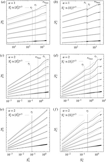
 ${\it\alpha}=2$
residual field defined by the procedure outlined in appendix B; they show markedly less intermittency than do the structure functions of the total field, with even the transverse velocity structure functions tending towards
 $n/3$
scaling in the inverse cascade.
(a,c,e) Longitudinal and (b,d,f) transverse velocity structure functions for (a–d) interstitial patches and (e,f)
 ${\it\alpha}=2$
residual field (
 ${\it\theta}_{thr}=2{\it\theta}_{rms}$
). (a,b)
 ${\it\alpha}=1$
and (c,d)
 ${\it\alpha}=2$
. They should be compared with the structure functions for the total field in figure 15(a,b) and (d,e). The forcing scale
 $r_{f}$
is marked by vertical dashed lines.

7. Conclusions
The purpose of this paper is to address a major unresolved problem in 2D turbulence: how well KLB similarity theory describes inverse cascades. In our simulations the forcing scale is well resolved and a direct cascade is present. We study how non-Gaussian and intermittent the inverse cascades are, and the role of vortices in their statistics, comparing 2D inverse cascades (
 ${\it\alpha}=1$
and
 ${\it\alpha}=2$
) where we expect KLB scaling to be realizable with an inverse cascade (
 ${\it\alpha}=3$
) where we do not. This study was partially motivated by the continuing lack of consensus on whether the
 ${\it\alpha}=2$
inverse cascade displays KLB scaling, is non-Gaussian and intermittent; we extend our study to include
 ${\it\alpha}=1$
, which corresponds to surface quasigeostrophic flow, and
 ${\it\alpha}=3$
, for which Burgess & Shepherd (Reference Burgess and Shepherd2013) predicted that an inverse-cascading inertial range with KLB scaling is non-realizable even if no vortices are present.
For all three systems the energy spectral slopes at inverse cascade scales are steeper than the KLB prediction. Because no large-scale drag or hypoviscosity is used and because we take data before appreciable energy builds up in
 $k=1$
, the steep spectra are not due to condensation or condensation-like effects. Coherent vortices, most larger than the forcing scale, are prominent in the
 ${\it\alpha}=1$
and
 ${\it\alpha}=2$
flows. This contrasts with previous results for
 ${\it\alpha}=2$
, which found no vortices larger than the forcing scale. For
 ${\it\alpha}=3$
vortices are few and small.
The one-point active scalar p.d.f.s have broad tails consistent with the presence of vortices; the tails are especially broad for
 ${\it\alpha}=1$
and
 ${\it\alpha}=2$
. The two-point active scalar p.d.f.s also have broad tails, and their shapes do not depend on scale. In contrast, the shapes of the two-point velocity p.d.f.s depend on scale, i.e. they indicate intermittency, with broad tails collapsing towards a more Gaussian shape at large scales. The variation in p.d.f. shape with scale is least pronounced for
 ${\it\alpha}=3$
. For
 ${\it\alpha}=1$
and
 ${\it\alpha}=2$
the range of scales over which the two-point velocity p.d.f.s change shape includes the vortex-containing scales.
The structure functions of the total fields also indicate intermittency for
 ${\it\alpha}=1$
and
 ${\it\alpha}=2$
, falling below the
 $n/3$
scaling at higher orders, though the velocity structure functions for
 ${\it\alpha}=1$
are non-intermittent in the approximate range
 $[r_{I},r_{V_{max}}]$
. In contrast, the
 ${\it\alpha}=3$
structure functions follow the
 $n/3$
scaling at all orders, suggesting that this flow is much less intermittent. In general the degree of intermittency depends on the structure function, with transverse velocity structure functions exhibiting more striking departures from the
 $n/3$
scaling at higher orders.
To probe the role of the vortices in the steep observed spectra, we used the continuous wavelet transform to compute spectrograms for the comparatively weak interstitial flow in between the large vortices. We found that the interstitial fields displayed approximate KLB energy-spectrum scalings
 $-2$
and
 $-(5/3)$
for
 ${\it\alpha}=1$
and
 ${\it\alpha}=2$
respectively. For
 ${\it\alpha}=1$
the interstitial longitudinal velocity structure functions are non-intermittent approximately over the range
 $[r_{f},r_{I}]$
, and for
 ${\it\alpha}=2$
they are non-intermittent over the range
 $[r_{f},r_{V_{max}}]$
. The residual field defined for
 ${\it\alpha}=2$
via thresholding and smoothing was also non-intermittent as measured by the longitudinal velocity structure functions, which displayed remarkable scaling properties. The transverse velocity structure functions of this residual field also tended towards
 $n/3$
scaling. This demonstrates the presence of a background flow with KLB scaling and which satisfies, to some extent, the non-intermittency assumptions of KLB mean-field theory.
The lack of vortices for
 ${\it\alpha}=3$
is evidence that the steep spectrum in this case is not due to coherent vortices but to non-realizability of an inverse cascade with KLB scaling, as predicted by Burgess & Shepherd (Reference Burgess and Shepherd2013). In fact, the energy spectral slope observed is close to the equipartition spectrum
 $-2$
. Both the KLB solutions and equipartition distributions are power law solutions to the EDQNM closure – our results suggest that when the inverse cascade cannot reach the KLB solution it tends to that of the enstrophy equipartition solution instead.
In summary, we have shown for
 ${\it\alpha}=1$
and
 ${\it\alpha}=2$
that turbulence forced at intermediate scales, leaving room for an enstrophy cascade, develops a non-Gaussian and intermittent inverse cascade populated by vortices and having a total spectrum steeper than the KLB prediction. Using continuous wavelets we showed that the interstitial field between the vortices displays KLB scaling for both
 ${\it\alpha}=1$
and
 ${\it\alpha}=2$
, as well as non-intermittent ranges in the longitudinal velocity structure functions.
In contrast to
 ${\it\alpha}=1$
and
 ${\it\alpha}=2$
, the turbulence for
 ${\it\alpha}=3$
is close to Gaussian and non-intermittent even for resolved forcing. The spectral slope is steeper than the KLB prediction and close to the enstrophy equipartition slope
 $-2$
. This suggests the inverse cascade simulated for
 ${\it\alpha}=3$
is close to the Gaussian and scale-invariant enstrophy equipartition solution, the other power law solution to the EDQNM closure calculated by Burgess & Shepherd (Reference Burgess and Shepherd2013).
To what extent KLB similarity theory describes 2D inverse cascades appears to be a rather complex question. Sensitivity to simulation parameters, the various tendencies of 2D fluids to form coherent structures, and the realizability of the KLB similarity solutions as inverse cascades all impact the answer. Though coherent structures form when flows with
 ${\it\alpha}=1$
and
 ${\it\alpha}=2$
are forced at resolved scales, causing spectral steepening, non-Gaussianity and intermittency, KLB theory remains a good description of the interstitial fields in these systems.
Acknowledgements
Funding was provided by the Natural Sciences and Engineering Research Council of Canada. B.H.B. was also supported by an Amelia Earhart Fellowship from the Zonta International Foundation while this research was being carried out. We would like to thank N. Kevlahan for very helpful comments and for suggesting the use of continuous wavelets. B.H.B. would like to thank J. Braden for useful discussions regarding the application of masks to fields with complex spatial structure. We also thank three anonymous reviewers for their helpful comments on the manuscript, and particularly referee 3, who suggested the argument presented in appendix A.
Appendix A
We estimate the time evolution of the integral scale
 $r_{I}$
defined in (4.5) following the argument given by Pouquet et al. (Reference Pouquet, Lesieur, Andre and Basdevant1975). Noting that the wavenumber of the energy spectral peak
 $k_{e}^{-1}$
follows approximately the same growth law as
 $r_{I}$
in the present simulations, we identify these two quantities. For an energy spectrum
 $$\begin{eqnarray}\mathscr{E}(k)=\left\{\begin{array}{@{}ll@{}}C_{1}(t)k^{5-{\it\alpha}},\quad & k<k_{e}(t),\\ C_{2}k^{-n},\quad & k_{e}(t)<k<k_{f},\end{array}\right.\end{eqnarray}$$
with
 $n>0$
assumed to be independent of time,
 $C_{1},C_{2}>0$
, and
 $k_{e}\ll k_{f}$
, the energy is approximately
 $$\begin{eqnarray}\displaystyle E & \simeq & \displaystyle \int _{0}^{k_{f}}\mathscr{E}(k)\text{d}k\nonumber\\ \displaystyle & \simeq & \displaystyle \frac{{\it\alpha}-n-5}{(6-{\it\alpha})(1-n)}C_{2}k_{e}^{-n+1},\end{eqnarray}$$
where we have used
 $C_{1}k_{e}^{5-{\it\alpha}}=C_{2}k_{e}^{-n}$
.
Since energy is injected at a constant rate
 ${\it\varepsilon}_{I}$
and the simulations start from a state of no flow, i.e.
 $E(t=0)=0$
,
 $$\begin{eqnarray}E\simeq {\it\varepsilon}_{I}t.\end{eqnarray}$$
Equations (A 2) and (A 3) yield
 $$\begin{eqnarray}\displaystyle & k_{e}\propto t^{1/(1-n)}, & \displaystyle\end{eqnarray}$$
 $$\begin{eqnarray}\displaystyle & r_{I}\propto t^{1/(n-1)}. & \displaystyle\end{eqnarray}$$
 $n=(7-{\it\alpha})/3$
and
 $$\begin{eqnarray}\displaystyle & k_{e}\propto t^{3/({\it\alpha}-4)}, & \displaystyle\end{eqnarray}$$
 $$\begin{eqnarray}\displaystyle & r_{I}\propto t^{3/(4-{\it\alpha})}, & \displaystyle\end{eqnarray}$$
 ${\it\alpha}$
increases. Deviations from KLB scaling modify these growth laws.
Appendix B
To globally define coherent and residual fields we used a simple combination of thresholding and smoothing. After identifying candidate coherent regions with
 ${\it\theta}>{\it\theta}_{thr}$
, where
 ${\it\theta}_{thr}$
is the threshold, we retained in the coherent field regions in which the peak value of the active scalar field exceeds a critical level
 ${\it\theta}_{\text{c}}$
. The purpose of the second threshold is to ensure that the structures selected are actually vortices with a sharp peak. The initial coherent field is defined by
 $$\begin{eqnarray}{\it\theta}_{coh}=\left\{\begin{array}{@{}ll@{}}0,\quad & |{\it\theta}|<{\it\theta}_{thr},\\ 0,\quad & |{\it\theta}|>{\it\theta}_{thr},~|{\it\theta}_{max}^{region}|\leqslant {\it\theta}_{\mathit{c}},\\ {\it\theta},\quad & |{\it\theta}|>{\it\theta}_{thr},~|{\it\theta}_{max}^{region}|>{\it\theta}_{\mathit{c}}.\end{array}\right.\end{eqnarray}$$
Removing the vortices leaves gaps in the residual field; to fill these gaps and remove sharp discontinuities from the residual field, we smooth the coherent field defined in (B 1) by convolution with a 2D low-pass filter. The residual field is then defined as
 $$\begin{eqnarray}{\it\theta}_{res}={\it\theta}-{\it\theta}_{coh}^{sm}.\end{eqnarray}$$