2. Three-dimensional stability of a counter-rotating vortex pair in a rotating fluid

In this section, the three-dimensional stability of a counter-rotating vertical vortex pair in a rotating fluid is analysed as a function of the rotation rate, starting from the well-known non-rotating limit (Leweke, Le Dizès & Williamson Reference Leweke, Le Dizès and Williamson2016). The effects of the viscosity and the separation distance between the two vortices will also be investigated.

2.1. Methods

We use the Navier–Stokes equations for an incompressible fluid with constant density $\rho _0$ in a frame rotating about the vertical axis $\boldsymbol {e}_z$ at rate $\varOmega _b$:

(2.1)$$\begin{gather} \partial_{t} \boldsymbol{u}+ \boldsymbol{u} \boldsymbol{\cdot}\boldsymbol{\nabla}\boldsymbol{u}+2\varOmega_b \boldsymbol{e}_z \times \boldsymbol{u} ={-} {\rho_0}^{{-}1} \boldsymbol{\nabla}p + \nu \Delta \boldsymbol{u}, \end{gather}$$

(2.2)$$\begin{gather}\boldsymbol{\nabla}\boldsymbol{\cdot} \boldsymbol{u} = 0, \end{gather}$$

where $\boldsymbol {u}=(u_x,u_y,u_z)$ is the velocity, $p$ is the pressure, $\nu$ is the viscosity and $(x,y,z)$ are the Cartesian coordinates.

To perform the stability analysis, a base flow consisting in a quasi-steady vortex pair has first been computed by integrating the two-dimensional Navier–Stokes equations initialized by two counter-rotating Lamb–Oseen vortices with circulations $\pm \varGamma$ and radius $R_0$, separated by a distance $b$ along the $y$ direction. In the following, the length and time units will be taken as $R_0$ and $2{\rm \pi} R_0^2/\varGamma$, respectively. The numerical code uses a pseudo-spectral method with periodic boundary conditions (Deloncle, Billant & Chomaz Reference Deloncle, Billant and Chomaz2008). Most of the aliasing errors are eliminated by truncating $95\,\%$ of the modes along each direction. Time advancement is carried out with the fourth-order Runge–Kutta scheme for the nonlinear term and exact integration for the viscous and diffusive terms. The time step is $\delta t= 0.02$. The horizontal size of the computational domain is chosen sufficiently large, $L_x=120,\ L_y=60+b$, in order to minimize the effects of the periodic boundary conditions. Such a large non-square domain is necessary because the eigenmodes exhibit wide wave trains in the $x$ direction for large rotation rate. The resolution used is $1024\times 640$. The Reynolds number and the separation distance have been always set to $Re =\varGamma /(2{\rm \pi} \nu )=500$ and $b=4$, except in § 2.2.2 when studying the effect of $b$ and viscous effects.

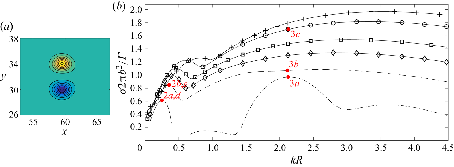
At time evolves, the two vortices quickly adapt to each other and reach a quasi-stationary state in which the vortex pair propagates at constant speed (Sipp, Jacquin & Cossu Reference Sipp, Jacquin and Cossu2000). Hence, the flow is quasi-steady in the reference frame travelling at that speed. The base state used for the following three-dimensional stability analysis has been taken as the flow at time $t=30$ (figure 1a). The characteristics of the vortices at that time have been obtained by fitting the vorticity field by the least-squares method to two Lamb–Oseen vortices with circulations $\pm\ \varGamma$ and separation distance $b$. For example, for $b=4$ and $Re=500$, this gives $R=1.12$, which is very close to the value given for a single diffusing Lamb–Oseen vortex $R=\sqrt {1+4\times 30/Re}\simeq 1.11$. For each different base state, the radius $R$ has been determined by this method.

Figure 1.

(a) Vertical vorticity of the base flow $\omega _{zb}$ for $b=4$ and $Re=500$. The contour level is $0.24$. (b) Non-dimensional growth rate ${\sigma } 2{\rm \pi} b^2/\varGamma$ as a function of the axial wavenumber ${k} R$ for $b=4$, $Re=500$ and various Rossby numbers: $Ro=\infty$ (– $\cdot$ –), $Ro=25.55$ (– – –), $Ro=17$ (—$\diamond$—), $Ro=12.75$ (—$\square$—), $Ro=8.50$ (—$\circ$—) and $Ro=6.38$ (—$+$—). The labels near the red points indicate the figure number where the corresponding eigenmode is displayed. The symbols are used only to distinguish each curve and do not represent all the data.

Using the same pseudo-spectral code, equations (2.1)–(2.2) linearized around the basic state have then been integrated for each axial wavenumber $k$ with a white noise as initial condition and with the same horizontal resolution, i.e. $1024\times 640$. After a sufficiently long integration time, the perturbation consists solely in the eigenmode with the largest growth rate. Several tests using different resolutions, time steps and box sizes have been carried out in order to check the accuracy of the computations. As seen in the example given in table 1, the growth rate only varies after the fourth significant digit when the box size is doubled, the resolution being fixed (fourth column) or when the resolution is doubled while keeping the box sizes constant (seventh column). The stability of a vortex pair at time $t=60$ has also been computed for one set of parameters. The growth-rate curves obtained for the latter time and $t=30$ differ by less than $2\,\%$, demonstrating the independence of the results with respect to the particular time chosen for the base flow.

Table 1.

Non-dimensional growth rate $\sigma 2{\rm \pi} b^2/\varGamma$ when the domain sizes are varied keeping the mesh sizes fixed (columns two to four) and when the mesh sizes are varied while keeping the box sizes constant (columns five to seven) for $b=4$, $Re=500$, $Ro=0.8$ and $kR=0.00448$.

2.2. Results

2.2.1. Effect of the rotation rate

Figure 1(b) shows the growth rate ${\sigma }$ non-dimensionalized by the strain $\varGamma /2{\rm \pi} b^2$ of the most unstable mode as a function of the vertical wavenumber $k$ non-dimensionalized by the vortex radius $R$ for different Rossby numbers defined as

(2.3)\begin{equation} Ro=\frac{\varGamma}{2{\rm \pi} R^2\varOmega_b}. \end{equation}

When $Ro=\infty$, there are several independent peaks (dashed dotted lines). The peak at low wavenumber corresponds to the well-known long-wavelength Crow instability (Crow Reference Crow1970). The dominant wavenumber is $kR \simeq 0.246$, giving a dominant wavelength $\lambda \simeq 7.2b$ in agreement with the scaling of Crow's theory (Crow Reference Crow1970). The maximum growth rate $\sigma \simeq 0.6 \varGamma /(2{\rm \pi} b^2)$ is slightly lower than inviscid Crow's theory because $Re$ is moderate. 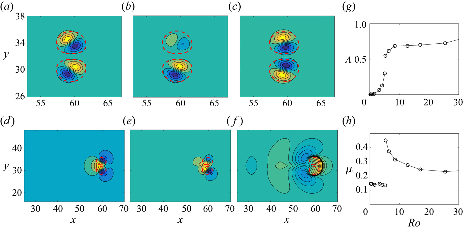The vertical vorticity $\omega _z$ of the dominant eigenmode (figure 2a) displays a dipolar structure in each base vortex. Such perturbation will displace the two vortices as a whole symmetrically as expected for the Crow instability. The second growth-rate peak around $k R\simeq 0.9$ (figure 1b) is small and corresponds to an oscillatory instability due to the resonance of azimuthal waves $m=0$ and $m=2$ with the strain (eigenmode not shown) as found for the Lamb–Chaplygin dipole (Billant, Brancher & Chomaz Reference Billant, Brancher and Chomaz1999). The third and fourth peaks for $k R=2.13$ and $k R=3.7$ are related to the first and second antisymmetric modes of the elliptic instability (Kerswell Reference Kerswell2002; Leweke et al. Reference Leweke, Le Dizès and Williamson2016) (see the first mode in figure 3a). These wavenumbers agree with the theoretical values predicted for a weakly strained Lamb–Oseen vortex in inviscid fluid: $kR=2.26$ and $kR=3.96$ (Sipp & Jacquin Reference Sipp and Jacquin2003; Leweke et al. Reference Leweke, Le Dizès and Williamson2016). The differences are probably due to viscous effects and finite ellipticity. The viscous effects also explain why the maximum growth rate of the first elliptic peak $\sigma = 0.97 \varGamma /(2{\rm \pi} b^2)$ is lower than the inviscid theoretical prediction $\sigma =9/16\epsilon =1.41 \varGamma /(2{\rm \pi} b^2)$, where $\epsilon =2.52\varGamma /(2{\rm \pi} b^2)$ is the internal strain rate in the case of the Lamb–Oseen vortex (Sipp & Jacquin Reference Sipp and Jacquin2003; Leweke et al. Reference Leweke, Le Dizès and Williamson2016).

Figure 2.

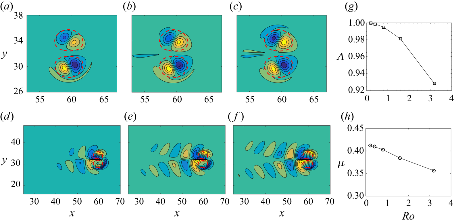
Vertical vorticity (a–c) and vertical velocity (d–f) of the eigenmode corresponding to the first growth-rate peak at low wavenumber for $b=4$, $Re=500$ and different Rossby numbers: (a,d) $Ro=\infty$, (b,e) $Ro=25.55$, and (c,f) $Ro=0.8$. (g) Asymmetry ratio $\varLambda$ and (h) ratio $\mu$ of the eigenmode of the first growth-rate peak as a function of $Ro$. The contour level is $0.24$ for (a–c), $0.025$ for (d,e) and $0.0074$ for (f). The eigenmode amplitude is normalized so that $\max (\vert \omega _z\vert )=1$. The red dashed lines are the isocontours where the basic state vorticity $\omega _{zb}$ is $0.05\max (\omega _{zb})$.

Figure 3.

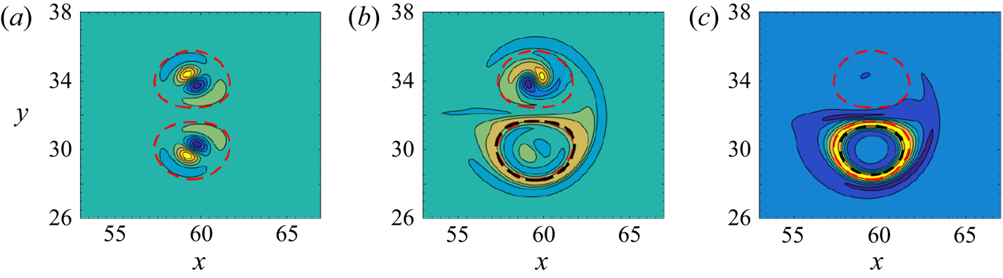
Vertical vorticity of the eigenmode for $k R=2.13$ for $b=4$, $Re=500$ and different Rossby numbers: (a) $Ro=\infty$, (b) $Ro=25.55$, and (c) $Ro=8.50$. The contour level is $0.24$. The red dashed lines are the isocontours where the basic state vorticity $\omega _{zb}$ is $0.05\max (\omega _{zb})$. The thick black dashed line in (b,c) represents the contour where $\omega _{zb}+2\varOmega _b$ changes sign.

When the background rotation is slightly increased such that $Ro=25.55$, the growth rate (dashed line in figure 1b) increases for all wavenumbers and only two distinct peaks are then present. The vertical vorticity of the eigenmode associated with the growth-rate peak at low wavenumber is no longer purely symmetric (figure 2b): the dipolar structure is much weaker on the upper vortex, which is cyclonic. This means that the instability will displace almost only the anticyclonic vortex. This asymmetry can be analysed quantitatively by decomposing the vertical vorticity $\omega _z$ into symmetric and antisymmetric parts as follows:

(2.4a,b)\begin{equation} \omega_{zs}= (\omega_z(x,y)+\omega_z(x,2y_c-y) )/2, \quad \omega_{za}= (\omega_z(x,y)-\omega_z(x,2y_c-y) )/2, \end{equation}

where $y_c$ is the $y$ coordinate of the symmetry plane between the two vortices. The ratio $\varLambda =\int _{0}^{L_x}\int _{0}^{L_y} \omega _{zs}^2\,\mathrm {d}\kern0.06em x\,\mathrm {d} y/\int _{0}^{L_x}\int _{0}^{L_y} \omega _{z}^2\,\mathrm {d}\kern0.06em x\, \mathrm {d} y$ then varies from unity for a purely symmetric mode to zero for a purely antisymmetric mode. As seen in figure 2(g), $\varLambda$ drops from unity for $Ro=\infty$ to $\varLambda =0.73$ for $Ro=25.55$.

Similarly, the vertical vorticity of the eigenmode at larger wavenumbers $k R=2.13$ is no longer purely antisymmetric for $Ro=25.55$ (figure 3b): this time, the elliptic mode is stronger in the cyclonic vortex than in the anticyclonic vortex, whereas a weak band surrounds the core of the latter vortex. When the Rossby number is decreased from $Ro=25.55$ to $Ro=8.5$, this mode on the anticyclonic vortex becomes strong while the elliptic mode on the cyclonic vortex fades out (figure 3c). Concomitantly, the growth rate continues to globally increase monotonically in the band $kR=[1,4]$ (figure 1b) until $Ro\simeq 4.25$ and then it decreases and goes to zero around $Ro= 1.35\pm 0.05$ (not shown). As seen in figure 3(b,c), the mode on the anticyclonic vortex arises in the vicinity of the line where the absolute vorticity $\omega _{zb}+2\varOmega _b$ changes sign (thick black dashed line). As shown by Sipp & Jacquin (Reference Sipp and Jacquin2000) and Gallaire & Rousset (Reference Gallaire and Rousset2006), this is an inviscid criterion for the centrifugal instability in non-axisymmetric vortices in rotating fluids. The critical value $Ro \simeq 1.35$ is also in good agreement with the critical Rossby number $Ro=1$ predicted by this criterion for the stabilization of the centrifugal instability. Viscous effects are certainly responsible for the difference.

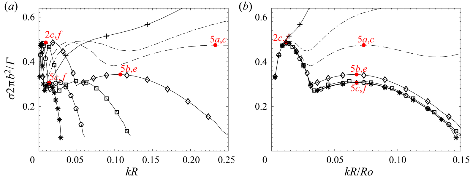
The growth-rate curves for smaller Rossby numbers down to $Ro=0.2$ are displayed on figure 4(a). Only a focus on small wavenumbers is shown. The growth rate for $Ro=6.38$ is plotted again to serve as reference (solid line with $+$ symbols). While the growth rate for any wavenumber was globally increasing as $Ro$ decreases when $Ro \geqslant 8.5$ (figure 1b), a different behaviour is observed in figure 4(a) when $Ro \leqslant 4.25$. Indeed, the growth-rate peak located around $k R \simeq 0.8$ for $Ro=6.38$ disappears but another peak emerges at lower wavenumber $k R\simeq 0.06$ for $Ro = 4.25$. As $Ro$ is further decreased, the maximum growth rate of this peak remains constant. In contrast, the corresponding most amplified wavenumber decreases dramatically as $Ro$ decreases. Rescaling $k R$ by $Ro$ (figure 4b), we can see that all the growth-rate curves collapse for low wavenumbers near the first peak. When $Ro \leqslant 0.8$, the collapse is almost perfect for the whole growth-rate curves. This proves that the vortex remains unstable to three-dimensional perturbations as $Ro \to 0$ but the dominant wavenumber scales like $Ro$. The maximum growth rate is $\sigma \simeq 0.5 \varGamma /(2{\rm \pi} b^2)$, i.e. of the same order as the maximum growth rate of the Crow instability in non-rotating fluid.

Figure 4.

Non-dimensional growth rate $\sigma 2{\rm \pi} b^2/\varGamma$ as a function of the axial wavenumber $kR$ (a) and $kR/Ro$ (b) for $b=4$, $Re=500$ and various Rossby numbers: $Ro=6.38$ (—$+$—), $Ro=4.25$ (– $\cdot$ –), $Ro=3.19$ (– – –) $Ro=1.59$ (—$\diamond$—), $Ro=0.8$ (—$\square$—), $Ro=0.4$ (—$\circ$—) and $Ro=0.2$ (—$*$—). See caption of figure 1(b) for other details.

The associated eigenmode is almost antisymmetric (figure 2c) and consists of a dipolar structure in each base vortex. Hence, this instability will displace the two vortices as a whole in antisymmetric directions. As displayed in figure 2(g), the asymmetry ratio behaves like $\varLambda \simeq 0.006 Ro^2$ for $Ro \lesssim 1$ so that the eigenmode tends to a purely antisymmetric mode when $Ro=0$. For $Ro \leqslant 3.19$, a second subdominant peak appears at slightly larger wavenumbers (figure 4a). The corresponding eigenmode resembles that of the first peak except that it is quasi-symmetric (figure 5) like for the Crow instability. The asymmetry ratio tends to unity as $Ro \to 0$ like $\varLambda \simeq 1- 0.008 Ro^2$ (figure 5g). It is also interesting to look at the vertical velocity field of these eigenmodes (figures 2f and 5d–f). Compared to $Ro=\infty$ (figure 2d), $u_z$ extends well outside the vortex cores and exhibits a wave train in the wake of the vortex pair (note the different scales in figures 2(d–f) and 5(d–f) compared to figures 2a–c and 5a–c). In addition, it is worth pointing out that the ratio between the maximum vertical and horizontal velocities,

(2.5)\begin{equation} \mu= \displaystyle{\dfrac{\max(\vert u_z\vert)}{\max\left(\sqrt{(u_x^2+u_y^2)/2}\right)}},\end{equation}

remains of order unity as $Ro$ goes to zero (figures 2h and 5h).

Figure 5.

Vertical vorticity (a–c) and vertical velocity (d–f) of the eigenmode corresponding to the second growth-rate peak for $b=4$, $Re=500$ and different Rossby numbers: (a,d) $Ro=3.19$, (b,e) $Ro=1.59$, and (c,f) $Ro=0.2$. The contour level is $0.24$ for (a–c) and $0.038$ for (d–f). (g) Asymmetry ratio $\varLambda$ and (h) ratio $\mu$ of the eigenmode of the second peak as a function of $Ro$. In (a–f), the red dashed lines are the isocontours where the basic state vorticity $\omega _{zb}$ is $0.05\max (\omega _{zb})$.

Even if we have focused on the region of small vertical wavenumbers in figure 4, we stress that we have not observed any other type of instability at higher wavenumbers when $Ro \leqslant 1$.

2.2.2. Effects of the separation distance and Reynolds number

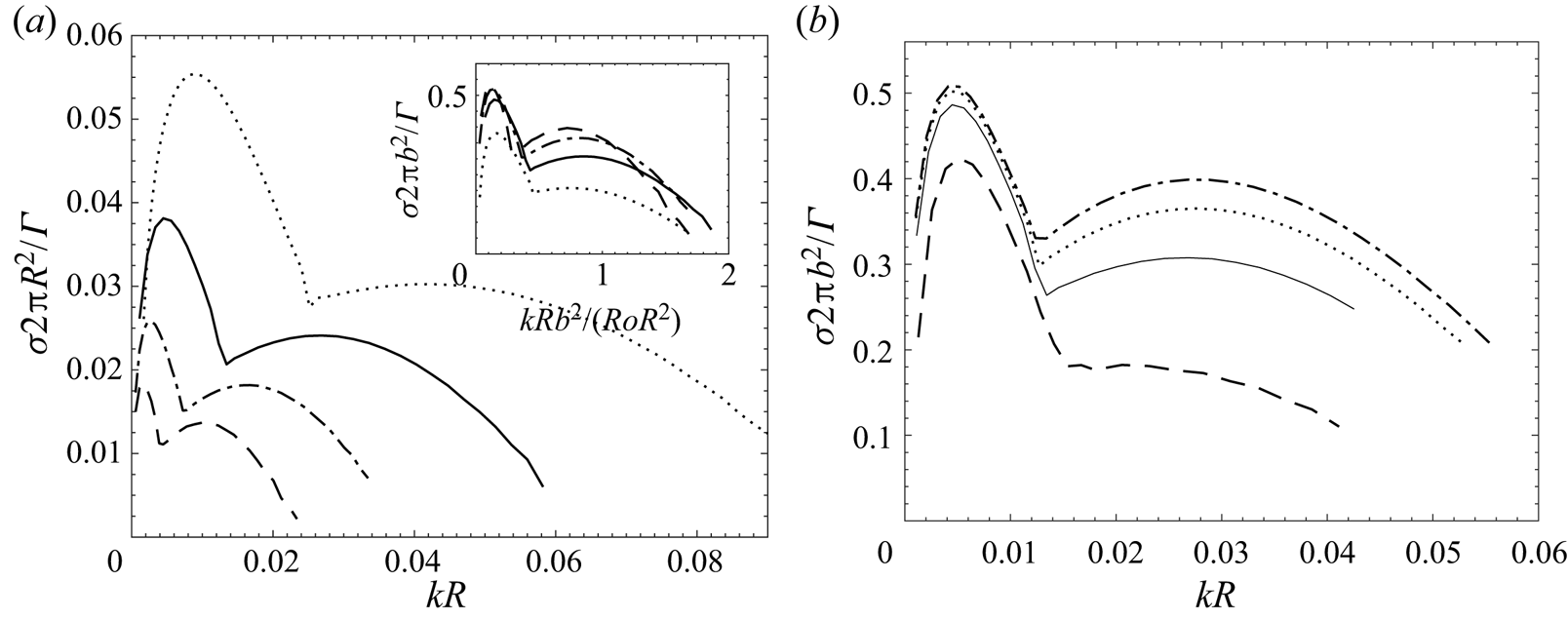
Figure 6(a) shows the growth rate non-dimensionalized by $\varGamma /2{\rm \pi} R^2$ for different separation distances $b$ for a fixed low Rossby number $Ro=0.4$, which belongs to the self-similar regime found above. The maximum growth rate of the two peaks and dominant wavenumbers decrease as $b$ increases, meaning that the instabilities weaken as the vortices are more distant. The inset in figure 6(a) shows the same curves but when the growth rate is rescaled by the strain and the wavenumber $k$ by $b^2/(Ro R)$. We can see that the growth-rate peaks are approximately aligned, indicating that, together with the dependence with the Rossby number found above, the dominant wavenumber scales like $Rk_{max} \simeq 0.15 Ro_b$, where $Ro_b= \varGamma /(2{\rm \pi} b^2\varOmega _b)$ is a Rossby number based on the separation distance $b$ instead of the vortex radius $R$. The corresponding wavelength scaling $\lambda _{max} \simeq 42 R/Ro_b$ differs from that of the Crow instability $\lambda _{max} \propto b$. Furthermore, the maximum growth rate of the Crow instability scales like the strain $\varGamma /(2{\rm \pi} b^2)$ while the inset of figure 6(a) shows that this scaling does not collapse the curves well. A better collapse, but still rather approximate, could be obtained by plotting $\sigma b^n$ with an exponent $n$ around $3/2$ (not shown). Similarly, the dominant wavelength associated with the subdominant growth-rate peak scales like $\lambda _{max} \simeq 7 R/Ro_b$.

Figure 6.

(a) Non-dimensional growth rate $\sigma 2{\rm \pi} R^2/\varGamma$ as a function of the axial wavenumber $kR$ for $Re=500$, $Ro=0.4$ and different separation distance: $b=3$ ($\cdots \cdot$), $b=4$ (——), $b=5$ (– $\cdot$ –) and $b=6$ (– – –). The inset displays the same curves in terms of the non-dimensional growth rate $\sigma 2{\rm \pi} b^2/\varGamma$ and wavenumber $kR b^2/(Ro R^2)$. (b) Non-dimensional growth rate $\sigma 2{\rm \pi} b^2/\varGamma$ as a function of $k R$ for $b=4$ and: $Re=200$, $Ro=0.30$ (– – –), $Re=500$, $Ro=0.4$ (——), $Re=1000$, $Ro=0.44$ ($\cdots \cdot$), and $Re=2000$, $Ro=0.47$ (– $\cdot$ –). In all cases, the rotation rate is fixed to $\varOmega _b=2$ but the Rossby number varies slightly since the radius $R$ increases as $Re$ decreases.

Finally, the effect of the Reynolds number is investigated in figure 6(b) for $b=4$ and a fixed rotation rate $\varOmega _b=2$ for which $Ro=0.4\pm 0.1$. The growth rate increases with $Re$ and tends to saturate to finite values as $Re$ becomes large, indicating that the instability is inviscid.

3. Direct numerical simulations

To complement the linear stability analyses, we have performed some DNS of the evolution of the quasi-antisymmetric displacement instability that is dominant for low Rossby number. The aims are to confirm that the instability does indeed lead to a three-dimensionalization of the vortex pair and to determine whether its nonlinear evolution continues to follow the same dependence on the Rossby number as that found in § 2. However, a detailed analysis of the nonlinear saturation mechanism is left for future studies.

These DNS have been carried out for two Rossby numbers $Ro=1.53$ and $Ro=0.76$ for the Reynolds number $Re=500$. The separation distance has been taken as $b=3$ because it leads to a smaller most amplified wavelength than for $b=4$ (see § 2.2.2) and thus requires a shorter computational domain in the vertical direction. For the sake of the computational cost, the horizontal sizes of the domain $L_x\times L_y$ have been reduced to $60\times 31.5$, keeping the same horizontal mesh sizes. Table 1 (column two) shows indeed that the growth rate varies by less than $1\,\%$ compared to the reference value obtained with the wider domain (column three).

The initial velocity field corresponds to the sum of the velocities of the base state and a perturbation consisting of the dominant eigenmode. The amplitude of the perturbation has been fixed such that its maximum vertical vorticity is $5\,\%$ of the maximum vertical vorticity of the base flow. The vertical size of the domain $L_z$ has been adjusted to the most amplified wavelength $\lambda _{max}$ for each Rossby number, i.e. $L_z=196.43$ for $Ro=1.53$ and $L_z=392.85$ for $Ro=0.76$. The mesh sizes have been set to be almost isotropic. Thereby, the resolutions are $N_x\times N_y\times N_z=512\times 320\times 1600$ for $Ro=1.53$ and $512\times 320\times 3200$ for $Ro=0.76$. The truncation has been reduced to nine-tenths of the modes along each direction. The convergence has been checked by increasing the resolution to $768\times 480\times 2400$ for $Ro=1.53$. The velocity at each point common to both resolutions have been found to differ by less than 1 % at any time.

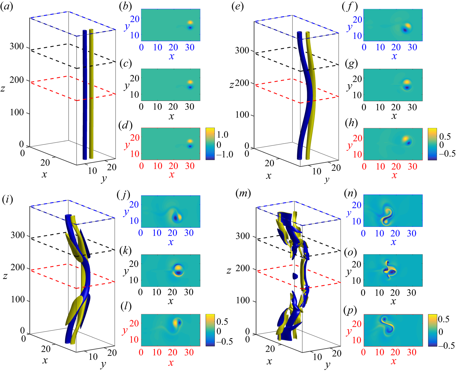
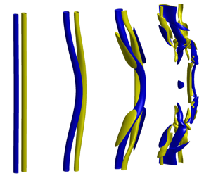
Figure 7 shows three-dimensional contours and horizontal cross-sections of the vertical vorticity for $Ro=0.76$ at different times. Supplementary movie 1 is available at https://doi.org/10.1017/jfm.2021.431. While the vortex pair looks straight at $t=0$ (figure 7a), since the perturbation is initially small, a vertical bending of the vortices becomes clearly visible at $t=100$ (figure 7e). In the horizontal cross-sections at $z=L_z/2$ (figure 7h) and $z=L_z$ (figure 7f), we see that the vortex pair propagates obliquely and symmetrically with respect to the $x$ direction. In contrast, the vortex pair continues to propagate in the $x$ direction at $z=3L_z/4$ (figure 7g). Such behaviour, which is consistent with the structure of the vertical vorticity of the eigenmode (figure 2c), is similar to that of the zigzag instability in strongly stratified fluid (Billant & Chomaz Reference Billant and Chomaz2000; Deloncle et al. Reference Deloncle, Billant and Chomaz2008). Note that the simulation is performed in the travelling reference frame where the vortex pair is steady at $t=0$. Since the vortex pair slows down due to viscous effects, it thus moves backwards in the $x$ direction in this reference frame.

Figure 7.

(a,e,i,m) Three-dimensional contours of the vertical vorticity $\omega _z$ at different times in a DNS for $Ro=0.76$, $b=3$ and $Re=500$. Yellow and blue contours represent, respectively, plus and minus 50 % of the vertical average of the maximum vertical vorticity in each horizontal plane. For each time, three horizontal cross-sections of the vertical vorticity in the planes $z=L_z/2$ (d,h,l,p), $z=3L_z/4$ (c,g,k,o) and $z=L_z$ (b,f,j,n) are displayed. The location of these cross-sections are also indicated by dashed lines with different colour in (a,e,i,m). The times shown are: (a–d) $t=0$, (e–h) $t=100$, (i–l) $t=130$, and (m–p) $t=160$. Note that only a portion of the computational domain is shown. The colorbar is the same for the three cross-sections at each time.

At $t=130$ (figure 7i), the vertical deformation has amplified and the vortex pair is now travelling in almost the opposite $y$ direction at $z=L_z/2$ (figure 7l) and $z=L_z$ (figure 7j). In between, at $z=3L_z/4$ (figure 7k), the vortex pair has kept its initial direction of propagation but two tongues of opposite vertical vorticity wrap the external part of each vortex. Such emergence of vertical vorticity is due to the stretching of the background vorticity by the vertical velocity, i.e. the term $2\varOmega _b\partial _{z} {u}_z$. The interactions between these tongues and the vortex cores initiate a breakdown of the vortex pair into smaller three-dimensional structures. Indeed, we see in figure 7(m), at $t=160$, that the vortex pair becomes fully three-dimensional and the initial vortex cores of the pair are strongly disorganized in the horizontal cross-sections (figure 7n–p).

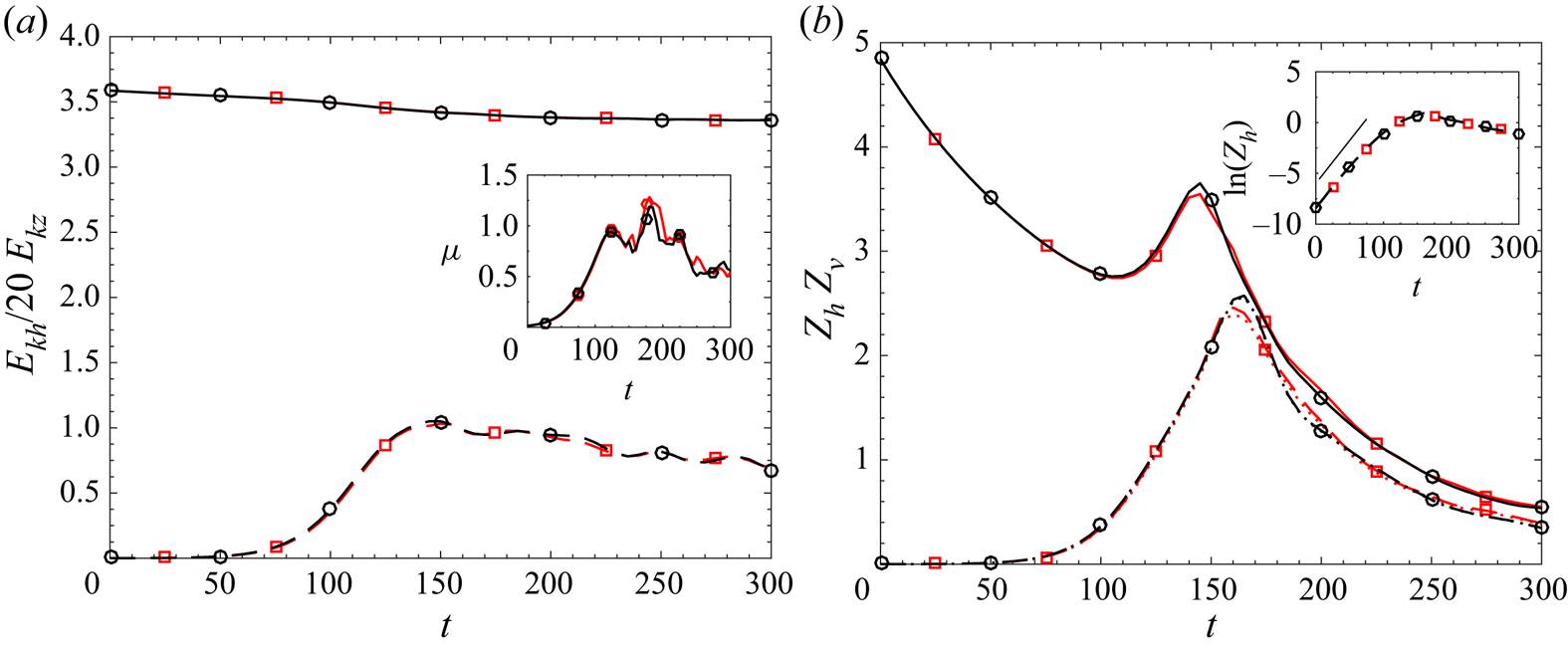
Figure 8(a) displays the evolutions of the total horizontal and vertical kinetic energies $E_{kh}=\langle u_x^2+u_y^2\rangle /2$ (divided by $20$ for convenience) and $E_{kv}=\langle u_z^2\rangle /2$, where $\langle \cdot \rangle =(1/L_z)\int _V \,\textrm {{d}}V$ is the volume integration per unit wavelength. In this way, these quantities are independent of the sizes of the computational box. The vertical kinetic energy (black dashed line with circle symbols) first grows exponentially and then saturates for $t > 150$ to a value of order unity. In contrast, the horizontal kinetic energy (black solid line with circle symbols) always slowly decays. Although the total horizontal kinetic energy is much larger than the vertical one, the inset in figure 8(a) shows that the ratio $\mu$ (see (2.5)) is of order unity at saturation, i.e. the maximum vertical and horizontal velocities are of the same order of magnitude.

Figure 8.

Evolution of the (a) kinetic energy and (b) enstrophy for two Rossby numbers, $Ro=0.76$ (black lines with circle symbols) and $Ro=1.53$ (red lines with square symbols), for $b=3$ and $Re=500$. In panel (a), the different lines correspond to horizontal and vertical kinetic energies $E_{kh}$ (——) and $E_{kv}$ (– – –). Note that $E_{kh}$ has been divided by a factor $20$. In panel (b), the lines represent vertical enstrophy $Z_{v}$ (——), horizontal enstrophy $Z_{h}$ (– – –) and $\langle (\partial _{y} u_z)^2+(\partial _{x} u_z)^2\rangle /2$ ($\cdots \cdot$). The inset in (a) represents the evolution of the ratio $\mu$ defined in (2.5). The inset in (b) displays the evolution of the logarithm of the horizontal enstrophy $Z_{h}$. The straight solid line represents an exponential growth at rate $2 \sigma$.

The corresponding evolutions of the total vertical and horizontal enstrophies $Z_{v}=\langle \omega _z^2\rangle /2$ and $Z_{h}=\langle \omega _x^2+\omega _y^2\rangle /2$ are shown in figure 8(b). The horizontal enstrophy $Z_h$ (black dashed line with circle symbols) grows exponentially until $t=160$. The inset in figure 8(b) shows that the growth rate of $Z_h$ is in good agreement with the linear stability analysis. The horizontal enstrophy saturates when reaching a value comparable to the vertical enstrophy $Z_v$ (black solid line with circle symbols) and then decays. In fact, the horizontal vorticity corresponds mostly to the horizontal shear of the vertical velocity, i.e. $\omega _x \simeq \partial _{y} u_z$, $\omega _y \simeq -\partial _{x} u_z$. Indeed, the black dotted line, which displays $\langle (\partial _{y} u_z)^2+(\partial _{x} u_z)^2\rangle /2$, is almost superimposed onto the curve of $Z_h$ (figure 8b). The vertical enstrophy, while decaying by viscous diffusion for $t < 100$, re-increases momentarily between $t \simeq 110$ and $t\simeq 150$. This is related to the appearance of the opposite vertical vorticity tongues (figure 7i).

The three-dimensional evolution of the vertical vorticity for the Rossby number $Ro=1.53$ is almost identical to that for $Ro=0.76$ (see supplementary movie 2). The evolutions of kinetic energies and enstrophies for $Ro=1.53$ are also plotted in figure 8 (red lines with square symbols). Remarkably, they are almost superimposed onto those for $Ro=0.76$. This demonstrates that the self-similarity evidenced in the linear stability analysis applies also to the nonlinear evolution of the instability. Altogether, this three-dimensional instability will therefore develop similarly whatever $Ro \lesssim 1$ in unbounded flows.

4. Scaling analysis

In § 2, we have found that the dominant wavelength of the three-dimensional instability of a counter-rotating vortex pair is inversely proportional to the Rossby number when $Ro \lesssim 1$. Here, we generalize this result by showing that this scaling derives from a self-similarity of (2.1)–(2.2) when the Rossby number is small. To this end, we consider a flow with characteristic horizontal and vertical velocity scales $U$ and $W$ and typical horizontal and vertical length scales $L_h$ and $L_v$. The Rossby number $Ro=U/(2\varOmega _bL_h)$ is assumed to be small and the fluid is considered to be unbounded. For the sake of clarity and simplicity, we consider an inviscid fluid, but it will be shown at the end that the following analysis applies equally to viscous flows.

In order to scale equations (2.1)–(2.2) with $\nu =0$, we define dimensionless quantities denoted with prime as follows:

(4.1a–g) \begin{align} \boldsymbol{u}_h &=U\boldsymbol{u}_h', \quad u_z=Wu_z', \quad p=2\rho_0\varOmega_bUp', \quad x=L_hx',\quad y=L_hy',\notag\\ z&=L_vz', \quad t=\displaystyle{\dfrac{L_h}{U}}t'. \end{align}

where the subscript $h$ is used to denote the horizontal components of any vector. The magnitude of the pressure has been fixed so as to balance the Coriolis force. The characteristic time scale has been chosen to be the advective time scale along the horizontal $L_h/U$. Such a hypothesis excludes fast inertial waves with typical frequency $O(\varOmega _b)$ but not those with a slow frequency of the order of $L_h/U$. The primes will be dropped in the following in order to keep the notation simple.

The resulting dimensionless equations are

(4.2)$$\begin{gather} Ro [\partial_{t} \boldsymbol{u}_h+\boldsymbol{u}_h\boldsymbol{\cdot}\boldsymbol{\nabla}_h \boldsymbol{u}_h +\alpha\delta u_z\partial_{z} \boldsymbol{u}_h ]+ \boldsymbol{e}_z \times \boldsymbol{u}_h ={-} \boldsymbol{\nabla}_h p, \end{gather}$$

(4.3)$$\begin{gather}Ro [\partial_{t} {u}_z+\boldsymbol{u}_h\boldsymbol{\cdot}\boldsymbol{\nabla}_h {u}_z +\alpha\delta u_z\partial_{z} {u}_z ]={-} \displaystyle{\dfrac{\delta}{\alpha}}\partial_{z} p, \end{gather}$$

(4.4)$$\begin{gather}\boldsymbol{\nabla}_h \boldsymbol{\cdot} \boldsymbol{u}_h+\alpha\delta \partial_{z} u_z = 0, \end{gather}$$

where $\alpha =W/U$ and $\delta =L_h/L_v$. It is also convenient to write the equation for the dimensionless vertical vorticity $\omega _z$:

(4.5)\begin{align} Ro [\partial_{t} \omega_z+\boldsymbol{u}_h\boldsymbol{\cdot}\boldsymbol{\nabla}_h \omega_z +\alpha\delta u_z\partial_{z} \omega_z ] = \alpha\delta [ Ro({\partial_{z} u_x \partial_{y} u_z-\partial_{z} u_y \partial_{x} u_z}+\omega_z\partial_{z} u_z )+\partial_{z} u_z ]. \end{align}

In the following, we further assume a priori that the vertical Rossby number is small,

(4.6)\begin{equation} Ro_v=\displaystyle{\dfrac{W}{2\varOmega_bL_v}}\equiv Ro\,\alpha \delta \ll 1, \end{equation}

but no other assumption on the individual orders of magnitude of $\alpha$ and $\delta$ will be used. This assumption together with $Ro \ll 1$ are sufficient to deduce the geostrophic balance from (4.2):

(4.7)\begin{equation} \boldsymbol{u}_h={-}\boldsymbol{\nabla}\times p\boldsymbol{e}_z +O (Ro, Ro_v ). \end{equation}

The vertical vorticity is therefore

(4.8)\begin{equation} \omega_z=\varDelta_h p +O ( Ro, Ro_v ).\end{equation}

and the divergence equation (4.4) becomes

(4.9)\begin{equation} \alpha\delta \partial_{z} u_z + O(Ro, Ro_v)=0. \end{equation}

Hence, (4.9) implies the order-of-magnitude relation

(4.10)\begin{equation} \alpha\delta \leqslant O(Ro), \end{equation}

confirming the hypothesis (4.6) since $Ro_v=Ro\,\alpha \delta \leqslant Ro^2$. By inserting (4.8) into the equation for the vertical vorticity (4.5) and by taking into account (4.10), we obtain at leading orders

(4.11)\begin{equation} Ro [\partial_{t} \varDelta_h p+\boldsymbol{u}_h\boldsymbol{\cdot}\boldsymbol{\nabla}_h \varDelta_h p ]=\alpha\delta\partial_{z} u_z +O (Ro^2). \end{equation}

By using (4.10), the momentum equation along the vertical, (4.3), can also be simplified to

(4.12)\begin{equation} Ro (\partial_{t} u_z+\boldsymbol{u}_h\boldsymbol{\cdot}\boldsymbol{\nabla}_h u_z ) ={-} \displaystyle{\dfrac{\delta}{\alpha}}\partial_{z} p + O (Ro^2). \end{equation}

Remarkably, this equation combined with (4.11) close the problem and allow one to find the leading-order solution in terms of $(p,u_z)$. Hence, the system has been reduced from four equations and variables to only two by simply using the two relations imposed by the geostrophic balance (4.7). It should also be pointed out that no a priori assumption on the magnitudes of $\alpha$ and $\delta$ has been necessary to derive these equations except (4.6).

As shown by Julien & Knobloch (Reference Julien and Knobloch2007) and Nazarenko & Schekochihin (Reference Nazarenko and Schekochihin2011), the application of the dominant balance or critical balance principles, respectively, to (4.11)–(4.12) implies $\alpha \delta =O(Ro)$ and $\delta /\alpha =O(Ro)$. Note that the critical balance principle imposes that the typical time scales of waves and advective motions should be of the same order (Nazarenko & Schekochihin Reference Nazarenko and Schekochihin2011). These principles both lead to $\alpha =O(1)$ and $\delta =O(Ro)$. However, the key point developed herein is that it is not necessary to invoke the dominant balance or critical balance principles to obtain these relations. They can be derived rigorously from an invariance of equations (4.11) and (4.12). Indeed, if we do not use these principles and still consider that $\delta$ and $\alpha$ are arbitrary and unknown, we can eliminate the Rossby number $Ro$, $\delta$ and $\alpha$ from (4.11) and (4.12) by the simple rescaling $\tilde {z} = zRo/\delta$ and $\tilde {u}_z=\alpha u_z$:

(4.13)$$\begin{gather} \partial_{t} \varDelta_h p+\boldsymbol{u}_h\boldsymbol{\cdot}\boldsymbol{\nabla}_h \varDelta_h p = \partial_{\tilde{z}} \tilde{u}_z, \end{gather}$$

(4.14)$$\begin{gather}\partial_{t} \tilde{u}_z+\boldsymbol{u}_h\boldsymbol{\cdot}\boldsymbol{\nabla}_h \tilde{u}_z ={-} \partial_{\tilde{z}} p, \end{gather}$$

so that all the non-dimensional parameters have disappeared. This rescaling gives the same scaling law for the vertical scale $L_v$ as the critical or dominant balances, $\delta =Ro$, i.e.

(4.15)\begin{equation} L_v \sim L_h/Ro. \end{equation}

Similarly, the rescaling of the vertical velocity is equivalent to stating that the orders of magnitude of the vertical and horizontal velocities are equal: $\alpha =1$, i.e. $W=U$. Therefore, the vertical length scale in rapidly rotating flows is set by a self-similarity of the equations for $Ro \ll 1$ like in strongly stratified fluids (Billant & Chomaz Reference Billant and Chomaz2001).

A posteriori, it is straightforward to remark that the above self-similarity continues to hold in the presence of viscous effects because the Laplacian of the viscous operator $\varDelta$ can be approximated by $\varDelta _h$ since $\delta ^2 \ll 1$. This explains why the scaling law (4.15) has been found to be well verified in § 2 even for a moderate Reynolds number $Re=500$.

The reduced equations (4.11)–(4.12), or equivalently (4.13)–(4.14), with the addition of viscous effects are identical to those obtained for rapidly rotating convection based on the dominant balance principle (Julien et al. Reference Julien, Knobloch and Werne1998; Julien & Knobloch Reference Julien and Knobloch2007) or for rotating turbulence by invoking the critical balance principle (Nazarenko & Schekochihin Reference Nazarenko and Schekochihin2011). Nevertheless, we believe that the present derivation based on a self-similarity is less heuristic and more general, thereby extending their range of applicability.

Besides the scaling law (4.15) for the vertical length scale, we emphasize that two other observations made in § 2 are fully consistent with this scaling analysis. First, the growth rate (figure 4b) and time evolution (figure 8) are independent of the Rossby number for low Rossby number, in agreement with the assumption that the characteristic time scale is $L_h/U$. Second, the ratio (2.5) is of order unity (figures 2h, 5h and 8a) consistently with the scaling $W=U$. Furthermore, these scaling laws imply $\omega _x = \partial _{y} u_z+O(Ro)$ and $\omega _y = -\partial _{x} u_z+O(Ro)$ as observed in § 3.