

1. Introduction
In recent decades, declining fertility and increasing life expectancy have caused a shrinking workforce and a rapidly growing retired population in advanced economies. The aging of the baby boom generation has amplified these trends. Everything else equal, when fewer productive workers must support a larger number of dependents, per capita output inevitably suffers. This simple arithmetic explains why many view population aging as a cause of secular stagnation. Other factors, however, may mitigate that negative outcome. Individuals may respond to aging by investing more in education, retiring later, and saving more. The latter may be an important force pushing down interest rates. In addition, firms may respond to those lower interest rates and also invest more. While these reactions reduce the negative impact of demographic change on per capita output, no evidence has been presented that they would lead to an overall positive outcome. More recently, however, Acemoglu and Restrepo (Reference Acemoglu and Restrepo2017) injected optimism into the discussion. Highlighting that firms can counteract the effects of a declining labor force by increased adoption of automation technologies, they suggested that aging does not contribute to secular stagnation. Other studies have confirmed the positive impact of automation on per capita growth (see below). However, they also introduced new concerns. If firms automate as an endogenous reaction to aging, this may also raise inequality. More specifically, the adoption of automation technology may erode the labor share of income and differences in the exposure to automation between individuals may imply rising wage inequality.
Our main objective is to reassess the net effect of demographic change on per capita economic growth, the labor share of income, and wage and welfare inequality, when firms can respond to aging by automating and when we account for the behavioral response of individuals. We tackle the following research questions. Can the increased adoption of available automation technologies by firms help economies avoid the negative effect of aging on per capita output? What are its welfare effects, and how are they distributed within and across generations of heterogeneous individuals? How can policy improve the effects of aging-induced automation in terms of macro efficiency and welfare inequality?
Answering these questions requires a quantitative theory which is realistic in the modeling of firms' adoption of automation, and which also gives room to the behavioral reactions of individuals to demographic change (in particular labor supply at older age and human capital formation). With respect to inequality, a promising analysis requires modeling individuals with heterogeneous skills. Our approach in this study is to construct, calibrate, and simulate an overlapping generations model for the United States that meets these standards (and that is also supported by a minimum of empirical evidence). It incorporates the characteristics just mentioned and adopts realistic exogenous patterns of fertility and life expectancy.
In more detail, as to automation, we integrate two strands of the automation literature, namely the task-based approach of Acemoglu and Restrepo (Reference Acemoglu and Restrepo2018a, Reference Acemoglu and Restrepo2018b) and the “two capital types” approach of Abeliansky and Prettner (Reference Abeliansky and Prettner2023) and Cords and Prettner (Reference Cords and Prettner2022). This theoretical innovation allows us to be more explicit about the precise channel through which aging stimulates automation. More specifically, we set up our model such that aging-induced automation takes the form of automated tasks substituting for non-automated tasks in a less-than-perfect manner, rather than capital substituting for labor perfectly in the execution of a given task. A key mechanism is that as the interest rate falls and wages rise as a result of demographic change, firms make more use of automated tasks at the expense of non-automated tasks executed by workers. Differences in the degree to which workers' tasks are substitutable, will make automation a driver of wage inequality. At the same time, our model acknowledges the typical role of traditional capital as a complement for all types of labor. As a result, we can study how aging affects investors' choice between “labour-replacing” and “labour-enabling” technologies (Frey, Reference Frey2019). The integration of two capital types into the task-based approach to automation is the first contribution of this paper.
By including a labor-education choice for young individuals, and a labor-leisure (retirement) choice for older individuals, we allow for key behavioral reactions of individuals to demographic change emphasized in the literature. While these reactions are known to reduce the negative impact of demographic change on per capita growth in standard macro models, their endogenization has not been seriously considered in the automation literature. In this article, the automation adjustment to aging, the behavioral adjustments to aging and their interaction are studied simultaneously in one integrated framework and we find that this is important. It is the second contribution of this paper.
Besides these two contributions, a clear strength of our paper is that we explicitly verify the empirical validity of our modeling choices regarding automation, labor supply at older age, and investment in education by the young. The related literature has largely neglected to do this. Before we use our calibrated model for simulations, we show that it can explain a large fraction of the cross-country differences in robotization.
Our main findings are as follows. First, aging strongly stimulates the adoption of automation technologies and the effect of aging on per capita output is much less negative if aging-induced automation is taken into account. In the long run we project that this negative effect may even disappear completely. Moreover, given our constant automation technology assumption, our results are to be seen as a lower-bound prediction: advances in automation technologies may generate faster, more complete mitigation of the negative effect. In contrast to the optimistic predictions of Acemoglu and Restrepo (Reference Acemoglu and Restrepo2017), among others, our simulations do leave, however, a foreseeable future of a few decades in which demographic change will constitute a force weighing down per capita output. Likewise, the aging-induced fall in the interest rate is softened by increasing automation, but not halted. One reason for why aging still affects growth negatively is that automated tasks are not perfect substitutes for tasks executed by human labor. Another reason is that aging-induced automation also raises the interest rate and thus reduces the strength of the behavioral reactions to aging: without aging-induced automation, the incentive to retire later and invest more in human capital accumulation would be stronger. Second, the partial mitigation of per capita output losses comes at the cost of heightened inequalities. In this respect we confirm existing literature. Aging-induced automation generates a fall in the labor share of income. And it increases welfare inequality between individuals of different innate ability levels. Third, policy matters. Although we expect aging-induced automation to bring aggregate welfare gains, these are unequally distributed. We find that ex-post redistribution is better than dissuading automation and limiting market inequality: the efficiency costs of a progressive income tax reform are far below those of halting the adoption of automation technologies.
Our paper belongs to a rapidly growing literature. Figure 1 provides an overview. Many papers have emphasized aging as a driver of secular stagnation, characterized by declining and persistently low per capita growth and interest rates. Some of these (and other) papers have highlighted the importance of counteracting behavioral effects via individuals' human capital investment and/or delayed retirement decision. Heer and Irmen (Reference Heer and Irmen2014) and Acemoglu and Restrepo (Reference Acemoglu and Restrepo2017) were among the earliest to study the endogenous response of automation and how this mitigates the adverse effects of a falling working-age population on per capita income. Many other papers followed, with some of them also showing that this mitigation comes at the price of rising inequality between workers and a falling labor share in income. The papers to which ours is most closely related are those of Basso and Jimeno (Reference Basso and Jimeno2021), Stähler (Reference Stähler2021), Irmen (Reference Irmen2021) and Zhang et al. (Reference Zhang, Palivos and Liu2022). We conclude that the findings of several recent studies (e.g., Irmen, Reference Irmen2021; Zhang et al., Reference Zhang, Palivos and Liu2022) regarding the mitigating role of automation in times of aging may be somewhat optimistic. Both the lower substitutability between automated and non-automated tasks and the negative interaction between automation and the behavioral reactions to aging explain why our results are less positive. In the light of our empirical validation, we judge both reasons to be credible. An important limitation is our assumption of constant automation technology. Firms may increasingly rely on automated tasks in our paper, but the fraction of tasks that are automatable and the overall efficiency with which automated tasks are executed, are constant. In that sense we differ from, among others, Heer and Irmen (Reference Heer and Irmen2014) who model technical progress as an endogenous outcome reinforced by labor scarcity. It explains why we called our results on future per capita output a lower-bound prediction.
Main mechanisms and literature to which this study contributes.

This paper is structured as follows. Section 2 sets out our model. In Section 3, we describe the parameterization and show the empirical relevance of the model. In Section 4, we simulate the impact of demographic change for the United States and we investigate how per capita output, other macroeconomic variables and welfare inequality would have evolved in the absence of aging-induced automation. We also consider how policymakers can better share the gains of automation in times of aging. Section 5 concludes.
2. The model
Our framework consists of a five-period overlapping generations model for a closed economy where hours worked at older age, human capital formation and the degree to which the production process is automated are endogenously determined. The set-up of the model also accommodates the study of inequality by allowing for heterogeneity in the innate ability of individuals within each generation. Furthermore, our model incorporates the empirical finding that the automatability of tasks falls unambiguously in the educational attainment of the individuals executing these tasks (Arntz et al., Reference Arntz, Terry and Ulrich2016; Frey & Osborne, Reference Frey and Osborne2017).
With regard to notation, we use superscript t to refer to the time period in which individuals enter the model. Individuals entering at time t will further on be called individuals “of generation t”. Subscript j is used to indicate that the generation is in the j-th period of their life and thus denotes the model age of an individual. Subscripts L, M and H refer to the three levels of innate ability: low, medium and high, respectively. Finally, time subscripts t that are added to aggregate variables indicate historical time periods.
2.1 Demography
In each model period, five different generations are alive: three active generations representing young, middle-aged and older workers, and two generations of retired individuals. Individuals enter the model when they become 20 years old and each period of life lasts for 15 years. Model ages j = 1, 2, 3, 4 and 5 thus correspond to actual ages 20–34, 35–49, 50–64, 65–79 and 80–94. Demographic change in the model is captured by time-varying fertility and life expectancy. Equation (1) indicates how the size of the generation of 20- to 34-year-olds alive at time $t\;( N_1^t )$ relates to the size of the young generation at time $t-1\;( N_1^{t-1} )$
 . n t is the time-varying fertility rate in the model. This approach follows, among others, de la Croix et al. (Reference de la Croix, Pierrard and Sneessens2013).

The survival of an individual from one period into the following is uncertain. We denote by $sr_j^t \;(\! < 1)$ the time-varying and age-dependent probability that an individual of generation t experiences utility in the j-th period of life, conditional upon having been alive in period j − 1. The size of generation t then evolves over time as described by equation (2).

The unconditional probability for an individual of generation t to reach the age group j is simply the product of the relevant conditional survival rates, as indicated in equation (3). Individuals in the fifth period of their life – aged 80 to 94 – die with certainty at the end of the period.

Each generation consists of individuals of low, medium, and high innate ability. It is assumed that fertility rates and survival rates do not vary over ability types and, in equation (4), that each ability group represents an equal share of each generation at every point in time.

The fertility rates and survival rates follow exogenous, country-specific trajectories throughout this study. Details on data sources and the construction of demographic parameters can be found in online Appendix C. There we also show that cross-country differences in the old-age dependency ratio are captured quite well by our model.
2.2 Production and the modeling of automation
A large number of identical firms operate on competitive markets for final goods, labor, and capital. The production function in equation (5) exhibits constant returns to scale in traditional physical capital K t and the total execution of tasks H t.

Equation (6) states that the total execution of tasks H t is a CES composite of the total execution of low ability, medium ability, and high ability tasks. The share term η a denotes the share of total tasks that are of the ability type a and s indicates how easily tasks of an ability type different from a substitute for tasks of ability type a in the production of final goods.

Equation (7a) indicates that the total execution of tasks of ability type a is, in turn, a CES composite of the execution of a continuum of tasks t a,i,t of that ability. Substitution between tasks of the same ability type is governed by the elasticity of substitution κ. In the spirit of Acemoglu and Restrepo (Reference Acemoglu and Restrepo2018a), tasks of ability type a with an index i smaller than or equal to ξ a are technologically non-automatable and can thus only be performed by assigning human labor of the ability type a to the execution of the tasks. Tasks of ability type a with an index i larger than ξ a are technologically automatable. This implies that automation capital (denoted by P t) is a perfect substitute for human labor of the ability type a in the execution of these tasks (with j and λ denoting their respective productivities). With l a,i,t, we denote the human labor assigned to the execution of the task of ability type a and index i in period t, while A t indicates human labor-augmenting technology. Note that our automation technology is of the general-purpose type as automation capital does not need to be assigned to a specific task, but inevitably executes any automatable task. It follows from our assumptions (explained in Appendix A, part 1) that it will be strictly cheaper for firms to make only use of automation capital for the execution of automatable tasks of any type such that $l_{a, i, t} = 0\;\;\forall i > \xi _{a\;\;}\;( {\forall a = L, \;M, \;H} )$ . This implies that, in our model, the share of tasks that is automated is constrained by technology (What tasks are automatable?) and not by the optimal choice of firms (Should I use capital or labor for the execution of this automatable task?). We are not the first to make this simplification in this context (Acemoglu & Restrepo, Reference Acemoglu, Restrepo, Agrawal, Gans and Goldfard2019). As a result of this simplification, all automatable tasks are fully automated in our model and equation (7a) can be simplified to equation (7b) (Appendix A, part 2).

with $\forall i \le \xi _a\colon \ t_{a, i, t} = A_tl_{a, i, t}\;$ and $\forall i > \xi _a\colon \ t_{a, i, t} = jP_t + {\rm \lambda }A_tl_{a, i, t}$

Equation (7b) expresses that the total execution of tasks of ability type a can be viewed as a CES composite of the execution of non-automated and automated tasks of type a, executed by human labor of type a (H a,t) and automation capital (P t) respectively. The model is neoclassical in nature in the sense that the sole source of long-run growth lies in labor-augmenting technical progress that is assumed to grow at a constant and exogenous rate x.

with 0 < ξ a < 1, with J = j (κ−1)/κ and with A t = A t−1(1 + x)
Finally, equation (8) describes total human labor of a specific ability type (H a,t). Human labor of different ages and the same ability type is assumed to be perfectly substitutable. As we explain in Section 2.4, n ja and h ja respectively denote hours worked and human capital of an individual of ability a and age j.

In this approach, two technological processes embodying automation coexist. (1) Automation at the extensive margin implies that more tasks become technologically automatable (captured by a rise in 1 − ξ a in the model). (2) Automation at the intensive margin follows from a rise in the productivity J of automation capital P for a given share of automated tasks 1 − ξ a. Firms will then substitute automated tasks for tasks executed by human labor. In this paper we assume automation technology (ξ a and J) to be constant, and therefore exclude these two processes.
We do allow, however, for non-technological automation. The same two types exist. Think of demographic change lowering the cost of capital relative to the cost of labor. First, non-technological automation at the extensive margin takes the form of firms using automation capital for the execution of automatable tasks that were executed by humans before. We also exclude this option in our model. We assume that all automatable tasks are already fully automated. Second, non-technological automation at the intensive margin implies that firms choose to make more use of automatable tasks, and less use of non-automatable tasks in their production process. For the low ability individuals, this non-technological automation at the intensive margin will lower the real hourly wage (cf. sub-section 3.1.6).
In our model, it is this non-technological automation at the intensive margin through which firms react to the change in factor costs implied by demographic change. This channel is very distinct from the true replacement of humans by automation capital in the execution of a given task, since it are tasks, not production factors that substitute for one another in the case of automation at the intensive margin. An example is in order to clarify this. The adoption of cost-effective computer technology entirely displaced the human computing profession. This is automation at extensive margin: a rise in 1 − ξ a implies that tasks which capital could not perform in the past are now only executed by capital due to the perfect substitutability between capital and labor in the execution of that task and the lower cost of executing that task using capital. Computers can do exactly the same computations, but in a far more cost-effective way than humans. Automation at the intensive margin happens when those tasks now performed by computers substitute, rather than complement for the tasks still performed by humans. High-speed computers still do not deliver the mail – this task itself is not automated –, but demand for this task has diminished due to the execution of tasks like e-mailing substituting for it.Footnote 1 Important to note is that, while we assume perfect substitutability between automation capital and human labor within the execution of an automatable task (as in Acemoglu and Restrepo (Reference Acemoglu and Restrepo2018b)), we consider automatable and non-automatable tasks of the same ability type a to substitute for one another in a less-than-perfect way. Sending an e-mail is an alternative to sending a postcard, but they are not interchangeable.
Finally, we want to highlight two important advantages of integrating the distinction between traditional capital K and automation capital P into the task-based framework of automation. It is not typical in task-based models of automation. We borrowed it from other frameworks of automation (Abeliansky & Prettner, Reference Abeliansky and Prettner2023; Cords & Prettner, Reference Cords and Prettner2022; Lankisch et al., Reference Lankisch, Prettner and Prskawetz2019). First, the presence of two capital types makes it possible for automation at the intensive margin to reduce the demand for (certain types of) labor. As argued by DeCanio (Reference DeCanio2016), q-substitutability between capital and labor is impossible in any production function with constant returns to scale and only two production factors. This is why – as acknowledged by Acemoglu and Restrepo (Reference Acemoglu and Restrepo2018b) – automation at the intensive margin will always raise the demand for labor in typical task-based models of automation with only two aggregate production factors (K and L). Since we have two types of capital in our model, the displacement of workers by automation technologies in our model can be envisaged both along the extensive and the intensive margin. A second advantage of distinguishing two capital types is that our model allows different effects on labor demand from different types of capital accumulation. Automation capital explicitly represents those instances in which the work performed by capital makes the work performed by labor less relevant for the production of final output. Following Acemoglu and Restrepo (Reference Acemoglu and Restrepo2018b), we mainly have computer-assisted machines, robotics, and artificial intelligence in mind when referring to automation capital. Traditional capital (e.g., infrastructure) then represents those, more typical, instances where capital empowers the relevance of human work and increases the demand for it.
2.3 Firm optimization
Equation (9) expresses the standard first-order condition that firms invest in traditional capital up to the point where its marginal product net of depreciation (δ k) is equal to the interest rate.

In equation (10), we impose that investment in traditional capital and automation capital yield precisely the same after-tax rate of return. This is what Abeliansky and Prettner (Reference Abeliansky and Prettner2023), Cords and Prettner (Reference Cords and Prettner2022) and Lankisch et al. (Reference Lankisch, Prettner and Prskawetz2019) refer to as the no-arbitrage condition. In this equation, τ p indicates the tax rate (τ p > 0) or subsidy rate (τ p < 0) that is applied to the marginal product of automation capital P t, with δ p its depreciation rate.

Labor markets are assumed to be perfectly competitive such that firms employ human labor of ability type a up to the point where the marginal product of effective human labor of type a equals the real hourly wage per unit of effective labor of individuals of that ability level. This condition is expressed in equation (11).

2.4 Individuals
2.4.1 Preferences
A representative individual of ability a and generation t experiences utility in the j-th period of life through the instantaneous utility function described in equation (12).

with $\gamma _1 = \gamma _2 = 0, \;\;\;\gamma _j > 0{\rm \;}\forall {\rm \;}j = 3, \;4, \;5$ and θ > 0 (θ ≠ 1)
Instantaneous utility is thus increasing in consumption $c_{ja}^t$ and leisure time $\ell _{ja}^t$
 experienced in that period. Preferences are logarithmic in consumption and iso-elastic in leisure with the intertemporal elasticity of substitution in leisure being 1/θ. γ j indicates the age-dependent utility value of leisure relative to consumption. Young and middle-aged individuals do not value leisure and, as a result, will opt to not allocate any time to leisure.
Each individual in the model maximizes their expected lifetime utility, described by equation (13). In this equation, β denotes the discount factor determining the present value of future utility, while $\pi _j^t$ has been defined in Section 2.1 as the unconditional probability to reach age j.

2.4.2 Time constraints
Every period is of the same fifteen-year length. We normalize this length to 1. Depending on the specific age and ability of an individual, time is allocated to either work (n), education (e) or leisure (ℓ). Equations (14) to (17) state the time constraints in each period.


Young individuals in equation (14) allocate their time to either work (n) or education (e). Individuals of low innate ability do not study when young $( e_{1L}^t = 0)$ . They are assumed to have zero productivity of schooling at the tertiary level. In later stages of life no one studies. Middle-aged individuals in equation (15) only work. Whereas young and middle-aged individuals have no leisure, retired individuals in their fourth and fifth period of life have only leisure, as expressed in equation (17). The statutory retirement age is 65. The generation of age 50 to 64 (j = 3) is the only generation in our model that is able to choose, in equation (16), what share $\ell _{3, a}^t$
 of time they allocate towards non-productive activities. Leisure time when older $\ell _{3a}^t$
 can be considered attainable through either reducing hours worked while still employed or through entering into early retirement schemes.
2.4.3 Budget constraints
Each individual enters the model with zero assets. Equations (18)–(20) state the budget constraints with which individuals of generation t are confronted in different periods of life.


Individuals allocate their disposable resources to either consumption $c_{ja}^t$ or the accumulation of non-human wealth. We denote by $\omega _{ja}^t$
 the stock of wealth held by an individual of ability a at the end of the j-th period of their life. Consumption is taxed at rate τ c. The right-hand sides of equations (18) and (19) show individuals' available resources during active life. These include after-tax labor income, non-employment benefits (only when older), non-human wealth accumulated in the previous period and the after-tax return on it, accidental inheritances (iht t) and lump-sum transfers from the government (tra t).
After-tax labor income rises in the real remuneration w a per unit of effective human labor provided by an individual of ability a, the human capital of that individual $h_{ja}^t$ , and the fraction of time spent working $n_{ja}^t$
 . It falls in the average tax rate on labor income τ wja. Since we model a progressive labor income tax system (cf. infra), tax rates depend on the ability and age of individuals. When older, at model age j = 3, individuals may choose to reduce their working time. In line with reality in many countries, they may then receive a benefit that is proportional to the time not spent working. This benefit can be thought to reflect both early retirement benefits (for those no longer working) and benefits in the context of phased retirement schemes (for older employees reducing work hours). The level of the benefit is a fraction of the net labor income an individual would receive if they worked. The policy parameter b indicates the net replacement rate.
If individuals survive into the next period t + 1, they lend out their unconsumed resources from period t to firms or the government. Individuals are paid back at the end of period t + 1 and remunerated at the after-tax real interest rate r(1 − τ ci), with τ ci a proportional capital income tax. At the end of the fifth period (80–94), all remaining individuals fully consume their remaining resources $( \omega _{5a}^t = 0)$ . This way, individuals in the final period of life do not die with debt nor do they willingly leave bequests. In other stages of life, individuals are allowed to have negative values $\omega _{ja}^t$
 .
During retirement, in equation (20), an individual receives old-age pension benefits, $pp_{4a}^t$ and $pp_{5a}^t$
 . The pension system in the model is of the pay-as-you-go type. Equation (21) describes the formation of these benefits as a function of the individual's net labor income in the past. The replacement rate is denoted by ρ. We impose that each of the three periods of active life are equally important for the calculation of the pension assessment base.

Finally, if individuals do not survive the transition to the following period, the unconsumed part of their disposable resources is not lent out to firms in the next period. In equation (22), IHT t indicates the total mass of unconsumed resources at the end of period t of individuals who do not reach the next period of their life. This total inheritance mass IHT t will be immediately distributed on an equal basis among all individuals in the form of a lump-sum transfer. The inheritance per person at the end of period t (iht t) is given by equation (23)Footnote 2.


2.4.4 Human capital formation
Individuals of different ability enter the model with different initial levels of human capital. The human capital of young individuals of the high ability type is normalized to h 0. Young individuals of medium and low ability dispose of only a fraction ${\rm \varepsilon }_a$ of this level.

This heterogeneity in individuals upon entering the model can be thought to reflect both differences in innate ability at birth and heterogeneous learning outcomes in primary and secondary education. Neither h 0 nor ${\rm \varepsilon }_a$ varies across generations such that equation (24) is not a source of long-term growth or of fluctuations in the skill premium.
In the first period of life, medium and high ability individuals can allocate time to increasing their level of human capital (reflecting participation in tertiary education between the ages of 20 and 34). Equation (25) describes the human capital production function. It is identical to that of Bouzahzah et al. (Reference Bouzahzah, de la Croix and Docquier2002) and Buyse et al. (Reference Buyse, Heylen and Van de Kerckhove2017), among others. Equations (26) and (27) indicate that human capital never depreciates. We have in mind that learning by doing at work may counteract depreciation.


2.4.5 Optimality conditions for savings, education and work
Individuals in the model maximize their expected lifetime utility (equation 13) subject to the budget and time constraints (equations (14) to (27)) by optimally choosing consumption in each period of active life and the share of time spent working when aged 50 to 64. Medium and high ability individuals also choose the amount of time spent at educational activities when aged 20 to 34. The relevant optimality conditions are described in online Appendix E.
2.5 Government
The government budget constraint is set out in equation (28). Government spending consists of government consumption G t, non-employment benefits to older workers B t, expenditures on the pay-as-you-go pension system PP t, interest payments on public debt r tD t and lump-sum transfers to all living individuals TRA t. The government levies taxes on labor income T n,t, on consumption T c,t, on the return to non-human wealth T ci,t and on the returns to automation capital T p,t. Government consumption G t is wasteful: it does not enter in the production function nor in individuals' utility function. The share of final output that is allocated to consumption G t follows an exogenous path defined by the evolution of g. If the government sets specific targets on the evolution of public debt, it can adjust lump-sum transfers. The pension system is fully integrated into government accounts.


Following Guo and Lansing (Reference Guo and Lansing1998) and Boone and Heylen (Reference Boone and Heylen2019), the average tax rates on labor income τwjat are progressively determined by equation (37). In accordance with the reality in most countries, the social security contribution is proportional to income with rate sscr.

Here, $w_{a,t}h_{ja}^{t + 1-j} n_{ja}^{t + 1-j}$ is the total pre-tax labor income of the individual at time t, and $\bar{y}_t^{lab}$
 is the average pre-tax labor income in the economy at time t. Γ thus represents the average labor tax rate for an individual whose labor income is at the economy-wide average and ψ determines the progressivity of the tax system. Both tax parameters are time-invariant throughout this study. The relevant labor tax rates for the decisions of individuals are the marginal tax rates. As long as ψ > 0, the marginal tax rate in equation (38) is higher than the average tax rate.

2.6. Aggregate equilibrium
Aggregate equilibrium on the market for final goods is ensured by the equilibrium on the market for loanable funds expressed in equation (39). More precisely, equation (39) imposes that the aggregate stock of non-human wealth held by individuals in the economy Z t coincides with the total stock of traditional capital, automation capital and government debt. The interest rate r t ensures that equilibrium on the market for loanable funds is achieved.

3 Parameterization and empirical relevance
3.1 Parameterization
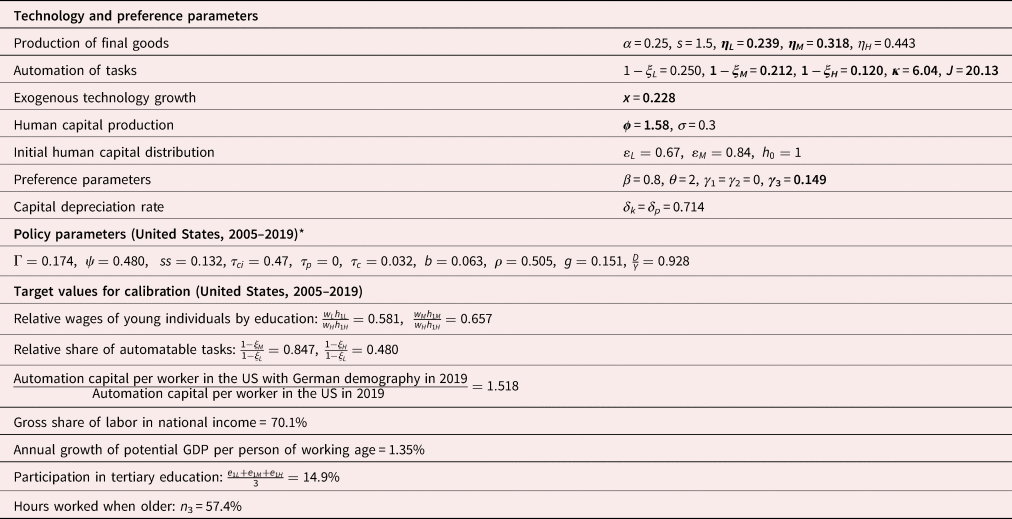
In order to evaluate our model's empirical relevance and to simulate the impact of exogenous shocks like demographic change, numeric values have to be assigned to the model's parameters. All parameter values in our baseline model can be found in Table 1. Nine parameters were calibrated to the US by imposing that the model perfectly replicates recent actual US data. In Table 1, these calibrated parameters are marked in bold. The other parameter values were taken from the literature. For more information on the construction of the calibration targets, we refer to online Appendix D. In the next section we evaluate the parameterized model's empirical validity by testing its capacity to explain cross-country differences in key outcome variables related to automation, education and labor supply.
Parameterization and target values for calibration

The parameters that were assigned a value through calibration on target values are marked in bold. For details on the definition, sources and construction of target values and policy parameters, we refer to online Appendix D.
* Until the period 2005–19, lump sum transfers adjust as the residual category in equation (28). From the period 2020–34 onwards, lump sum transfers per capita grow with the rate of exogenous human labor-augmenting technical progress (x) and the consumption tax rate τ c adjusts as the residual category in equation (28).
3.1.1 Technology and preference parameters
The rate of physical capital depreciation is assumed to be the same for traditional capital and automation capital. We impose δ k = δ p = 0.714, which implies a yearly depreciation rate of around 8% because of the fifteen-year length of one model period. Similarly, we impose β = 0.8, which reflects a rate of time preference of 1.5% per year. We assume the share parameter α for traditional capital in the production function for final goods to be equal to 0.25. The idea is that before tasks were technologically automatable $( \xi _a = 1, \;\forall a = L, \;M, \;H)$ , the share of capital in national income was constant and equal to the share parameter of the Cobb-Douglas production function α. This is thought to reflect the historical constancy of the labor share (Kaldor, Reference Kaldor, Lutz and Hague1961; Keynes, Reference Keynes1939). With regard to the level of the constant initial wage share, our value of 0.75 is consistent with the findings of Johnson (Reference Johnson1954) and Gollin (Reference Gollin2002).
The elasticity of substitution s between labor (tasks) of different ability types is set equal to 1.5. The empirical labor literature consistently documents values between 1 and 2 (Caselli & Coleman, Reference Caselli and Coleman2006). For the value of the intertemporal elasticity of substitution in leisure (1/θ) we follow Rogerson (Reference Rogerson2007). He puts forward a reasonable range for θ in macro studies from 1 to 3. In line with this, we impose θ to be equal to 2. This choice implies an elasticity of labor supply which is much higher than the very low elasticities typically found in micro studies. Given our macro focus, however, these micro studies may not be the most relevant ones (Fiorito and Zanella, Reference Fiorito and Zanella2012; Rogerson and Wallenius, Reference Rogerson and Wallenius2009). Several parameters in our model relate to human capital production. For the elasticity of human capital with respect to education time (σ) we choose a conservative value of 0.3. This value is within the range considered by Bouzahzah et al. (Reference Bouzahzah, de la Croix and Docquier2002) and Docquier and Paddison (Reference Docquier and Paddison2003). For the values of the relative initial human capital of medium and low ability individuals (relative to the initial human capital of high ability individuals, $\varepsilon _M$ and $\varepsilon _L$
 ), we follow Buyse et al. (Reference Buyse, Heylen and Van de Kerckhove2017). They looked at the distribution of PISA science test scores in OECD countries. From the robust pattern they observed in relative scores of weaker and median performers relative to better performers, they derived $\varepsilon _L = 0.67$
 and $\varepsilon _M = 0.84$
 . The initial level of human capital with which high ability individuals enter the model is normalized to one (h 0 = 1). We calibrated all remaining parameters by imposing that the model matches key recent data for the US.
The relative taste for leisure of individuals during the final period of active life (γ 3) is set to generate an employment rate among older workers, averaged over the three ability groups (n 3) of 57.4%. This is the fraction of potential hours that were actually worked by all individuals aged 50 to 64 in the US during the 2005–2019 period (for more details, see online Appendix D). The exogenous growth rate of A t is the only source of long-term per capita growth in the model, which is why x is set to match the average yearly growth rate of potential GDP per person of working age. This was 1.35% in the US for the years between 2005 and 2019, leading to a value of x of 0.228. We calibrate the efficiency parameter in the human capital production function ϕ such that the model accurately predicts the 2005–2019 data on the average aggregate participation in education of individuals between 20 and 34.
For the calibration of the share parameters of the three different ability types of labor (tasks) relevant to the production of final output (η L, η M, η H), our target values are the pre-tax wages of young workers of low and medium education relative to the wages of young workers of high education. More specifically, we target data published by the OECD (Education at a Glance 2020) for the wages of 25- to 34-year-old individuals whose highest degree is of the upper secondary level or lower (ISCED 3 or lower) and of individuals with short-cycle tertiary education (ISCED 5), relative to the wages of individuals with at least a bachelor's degree (ISCED 6 or higher). This educational division best approximates our modeling assumption that individuals with low ability do not participate in tertiary education, while those of medium and high ability do.Footnote 3 This results in values for η L and η M respectively. The value for η H then follows as η H = 1 − η L − η M.
3.1.2 Automation parameters
We identify five parameters relating to automation. These are the shares of automatable tasks by ability type 1 − ξ a (for a = L, M, H), the elasticity of substitution between automatable and non-automatable tasks κ, and the productivity of automation capital J. They are determined such that our model replicates five facts or well-informed hypotheses. A first one is that 25% of tasks of low ability are automatable. A second and third are that the fractions of automatable tasks of medium and high ability equal respectively 85% and 48% of the fraction of automatable tasks of low ability. A fourth one is that due to automation the labor share in the US fell from 75% to about 70% in 2005–2019. The fifth one is the finding of Acemoglu and Restrepo (Reference Acemoglu and Restrepo2022) that if the demographic structure in the US were the same as in Germany, robot density in the US would be 52% higher. We now clarify these facts or hypotheses in greater detail.
3.1.3 Shares of automated tasks: 1 − ξ a for a = L, M, H
The basis of our calibration is the work of Arntz et al. (Reference Arntz, Terry and Ulrich2016) and Popescu et al. (Reference Popescu, Petrescu, Sabie and Muşat2018). Both studies reveal clear heterogeneity between ability types in the share of tasks 1 − ξ a that are automatable. Unlike most other studies, Arntz et al. (Reference Arntz, Terry and Ulrich2016) adopt a task-based approach to estimate the share of jobs and individuals at high risk of automation. This makes their results a more reliable point of reference for us to start from. More precisely, they report for the three groups in the US with the lowest ISCED levelsFootnote 4 estimated shares of workers at high risk of automation equal to 100%, 44%, and 19% respectively. Weighing these shares with the relative size of these three low education groups (US Census Bureau, Current Population Survey), we obtain that 25.3% of, what we label, low ability individuals are employed in highly automatable occupations. If we assume a one-to-one relationship between the task content of jobs and the education level of those who execute them, it follows that a share of 25% of low ability tasks are automatable (1 − ξ L).
Taking this 25% for 1 − ξ L as our benchmark, similar shares of tasks of medium and high ability that are automatable can be derived fairly easily from Popescu et al. (Reference Popescu, Petrescu, Sabie and Muşat2018). They build on the work of Frey and Osborne (Reference Frey and Osborne2017) and also estimate the probability of job automation by education level.Footnote 5 We impose that the relative levels of future automation probabilities that they report, are also reflected in the share of tasks of each ability that are already automated. In practice, this results in two conditions demanding that the share of medium ability (high ability) tasks that are automated is 84.7% (48.0%) of the share of low ability tasks that are automated. In absolute terms, it then follows that we impose a value for 1 − ξ M equal to 21% and a value for 1 − ξ H equal to 12%. We thus assume that the same ability bias expected in future automation has been present in the automation technologies up to now. Compared to the findings of Arntz et al. (Reference Arntz, Terry and Ulrich2016), Popescu et al. (Reference Popescu, Petrescu, Sabie and Muşat2018) put forward relatively small differences in job automatability between education levels. By opting for their estimates to serve as calibration targets, our model is conservative in the sense that it is less likely to overestimate the skill-biased effects of automation.
3.1.4 Efficiency parameter of automation capital J
With the three shares of automated tasks (1 − ξ a) fixed above, the efficiency parameter J determines the share of income that is a remuneration for automation capital (equation 40).

Since traditional capital K t and the total execution of tasks H t are combined in a Cobb-Douglas production function with an output elasticity of traditional capital of 0.25, the share of human labor in the national income is 0.75 minus automation capital's income share. As indicated earlier, before tasks became technologically automatable $( \xi _a = 1, \;\forall a = L, \;M, \;H)$ , automation capital's share of income was zero (equation 40) and the labor share of income was a constant 0.75. We then calibrate the constant parameter value J such that – with given values of 1 − ξ a and the demographic parameters – the labor share that our model produces in the US for the 2005–2019 model period is lower than this original 0.75 as a result of automation. More specifically, we will target a value for the US labor share in this period of 0.701. That is precisely half of the fall from the initial 0.75 to the level of 0.652 that Gutiérrez (Reference Gutiérrez2017)Footnote 6 finds for the US labor share (excluding the real estate, finance and non-business sectors) for 2010–2014. In imposing that the automation of tasks was the driving force behind 50% of the fall in the labor share, we are in line with the findings of Karabarbounis and Neiman (Reference Karabarbounis and Neiman2014), Dao et al. (Reference Dao, Das, Koczan and Lian2017) and Bergholt et al. (Reference Bergholt, Furlanetto and Maffei-Faccioli2022). This approach yields a value for J equal to 20.1.
We derive and discuss the inequality conditions that have to hold such that it is strictly cheaper for firms to execute automatable tasks by automation capital in Appendix A, part 1. For the value of J that we obtained, these conditions are satisfied for each ability level.
3.1.5 Elasticity of substitution between automated and non-automated tasks: κ
Our calibration imposes constant parameter values for 1 − ξ a and J over all periods. This choice reflects our focus on non-technological automation at the intensive margin, as argued in sub-section 2.3. In response to aging (increased life expectancy and scarcity of young workers), firms can substitute automated tasks for tasks executed by humans. The elasticity of substitution between automated and non-automated tasks κ is crucial in this respect. We calibrate κ such that aging induces automation to the extent that is found by the empirical study of Acemoglu and Restrepo (Reference Acemoglu and Restrepo2022). They find that if the US had the same demographic trends as Germany – keeping all other things equalFootnote 7 – “the gap in robot adoption between the two countries would be 50% smaller” (p. 2). Practically, we use the data for 2014 that Acemoglu and Restrepo (Reference Acemoglu and Restrepo2022) present on the size of the robotics gap between Germany and the US: Germany's relative lead in robotics was approximately 103.6%. Acemoglu and Restrepo (Reference Acemoglu and Restrepo2022) thus more generally find that if the US had the demographic structure of Germany, their robot density would be 51.8% higher (half of 103.6%). For our calibration, we therefore impose that applying German demography to the US and keeping all other things equal leads to a rise in the baseline automation density of 51.8% at the end of the 2005–2019 period. This is the target value for our calibration. It yields a value of κ equal to 6.04.
The explanation for why the longer life expectancy and the scarcity of workers in Germany relative to the US contribute to the higher adoption of robotics in Germany is twofold. Note that as automated and non-automated tasks substitute better for one another (a higher κ), both explanations for why aging stimulates automation gain in strength. First, the literature finds that increased longevity and reduced fertility have a net positive effect on total savings (e.g., Carvalho et al., Reference Carvalho, Ferrero and Nechio2016). In our closed economy model, increased national savings translate to lower interest rates and capital deepening for all types of capital. The fall in the cost of capital will result into automation capital deepening more so when κ is higher, since a higher elasticity of substitution with labor counteracts diminishing returns to capital (Palivos & Karagiannis, Reference Palivos and Karagiannis2010). Irmen (Reference Irmen2021) too finds that, in the long run, a rise in longevity stimulates automation. Second, Abeliansky and Prettner (Reference Abeliansky and Prettner2023) outline how a fall in fertility can generate a relative shortage of human labor supply that can encourage the adoption of automation technologies. While automation capital is only a q-substitute for low and medium ability labor (cf. infra), it can be shown that an equal fall in the labor supply of all ability types positively affects the marginal product of automation capital (while, of course, reducing the marginal product of traditional capital) for the calibrated parameter values. Given the no-arbitrage condition, a fall in fertility will thus stimulate the accumulation of automation capital.Footnote 8 The automation-enhancing effect of a fall in fertility will be stronger in case of a higher value for κ, since the derivative of the marginal product of automation capital with respect to the human labor input will be more negative in case of a higher κ.
3.1.6 Automation at the intensive margin and the effect on wages: q-substitutes?
In this sub-section, we show that our model succeeds in creating heterogeneous wage effects related to a rise in P (non-technological automation at the intensive margin) despite the common elasticity of substitution κ. The main driver of this result is the difference in the shares of total tasks that are automated 1 − ξ a. Equation (41), derived in Appendix B, determines whether a rise in the input of automation capital in the production function has a positive or negative effect on the real hourly wage per unit of effective labor for an individual of ability a. The continuity condition for symmetry of the mixed second order derivatives is met, such that equation (41) also indicates whether the marginal product of automation capital is decreasing or increasing in the amount of human labor of type a.

Equation (41) consists of two terms that have distinct interpretations. The first term indicates the effect of a rise in P on the wage of workers of ability a through the increased execution of automatable tasks of type a. This is the direct displacement effect. The degree to which automated tasks can substitute for non-automated tasks of the same ability type a – embodied by the elasticity of substitution κ – plays a crucial role here. For our calibrated parameter values, this first effect is negative for all ability types. It will be more negative for the low and medium ability workers, however, since a larger share of tasks performed by them are automated (larger 1 − ξ a). This is not the whole story though. The second term indicates the effect of a rise in P on the wage of workers performing tasks of type a through the increased execution of automatable tasks of a type different from a.Footnote 9 This is the indirect productivity effect. The elasticity of substitution s between the different ability types plays a large role in determining the sign of this second effect. For our calibrated parameter levels, tasks of different ability types are q-complements and the effect will be positive.
The net effect of this non-technological automation at the intensive margin is negative for low and medium ability workers, but positive for high ability workers given the calibration. Automation capital is thus only a q-substitute for low and medium ability human labor, since, for workers of high ability, the negative displacement effect of automation is more than fully compensated by the increased execution of complementary tasks.
3.2 Empirical test of the model
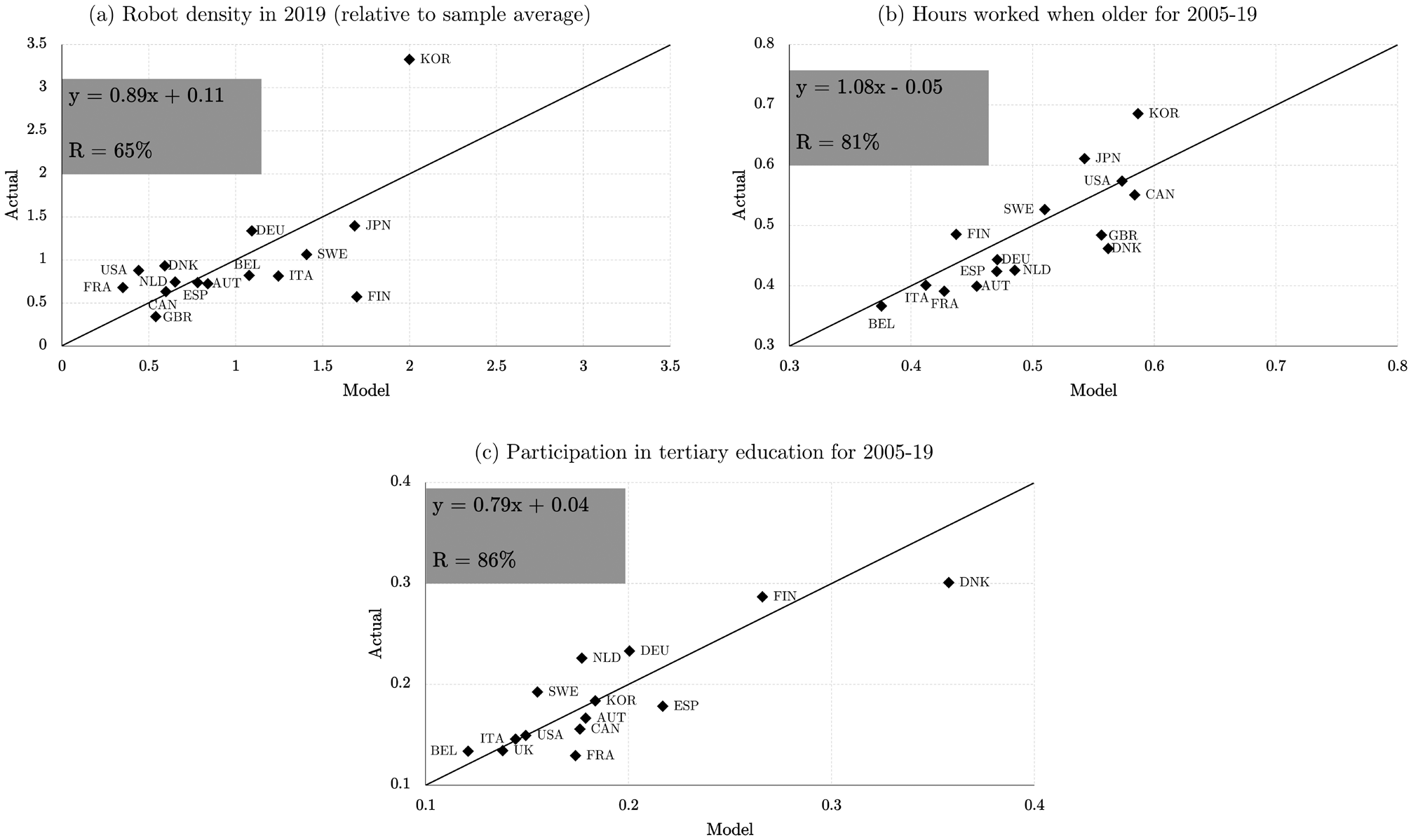
In this section we test whether the calibrated model succeeds in accurately mimicking key recent facts regarding the three discussed mechanisms through which the negative effect of aging on per capita output can be counteracted. We do this by confronting our model's predictions with the data on cross-country differences in automation, employment among older workers, and participation in tertiary education. Our calibration only implies that the model's predictions match the data exactly for the US such that an informative test of the model's validity and empirical relevance consists of verifying whether the model can also match the data for other OECD economies and the size of the cross-country differences. To do this test, we impose the preference and technology parameters reported in Table 1 for the US on all countries. Only the exogenous demographic variables and policy parameters differ between the different country versions of the model. In online Appendices C and D, we describe the demographic variables and the policy parameters in greater detail. The only “technology” parameter that differs between countries is the efficiency parameter ϕ in the production of human capital. Here we follow the approach in Boone and Heylen (Reference Boone and Heylen2019) and allow differences across four country-groups to capture the differences in institutions that may affect the characteristics of tertiary educationFootnote 10. All in all, this confrontation with the data in Figure 2 is encouraging. Our model translates observed differences in demography and policy into realistic performance differences regarding the three key endogenous counteracting mechanisms discussed in the introduction.
Model predictions (horizontal) against actual data (vertical). Underlying the model predictions for each country is the assumption that, until the period 2005–19, lump-sum transfers adjust in equation (28) to keep the predicted public debt-to-GDP ratio equal to its actual level. From the period 2020–34 onwards, lump sum transfers per capita grow with the rate of exogenous technical progress (x) and the consumption tax rate τ c adjusts as the residual category in equation (28).

The solid black line in each panel of Figure 2 is the 45°-line. In the upper left corner of each panel, we also report the specification of the regression line that provides the best linear fit between the model's predictions and the data, as well as the correlation coefficient. The regression line itself is not drawn. Figure 2(a) verifies whether the model can accurately reproduce differences in automation between countries. The actual data used comes from the report of the International Federation of Robotics (IFR) (2021).Footnote 11 The IFR presents data on robot density in the form of “number of industrial robots per 10,000 employees in the manufacturing industry”, out of which we select fifteen OECD economies. The vertical axis of Figure 2(a) shows the actual robot density in 2019, expressed relative to the sample average. The model's indicator of automation density – set out on the horizontal axis – is the ratio of the amount of automation capital P t at the end of the 2005–2019 period relative to the size of the three active generations in this period. Since everyone on the labor market actually works in the model, this indicator reflects the amount of automation capital per worker (of which some workers work full time and some part-time, as in reality). The values of this indicator are, for all fifteen OECD economies, also expressed relative to the sample average.
The baseline correlation between the model's predictions and the actual values in (a) is 65%. The slope of 0.89 is relatively close to the “optimal” value of 1. In other words, our model does not systematically overestimate the effects of demographic and policy differences by too much (slope below 1), nor does it systematically underestimate these effects (slope above 1). Even when we remove Korea from the sample, correlation is still a respectable 46%. The model accurately captures the high degree of automation in the two East Asian economies relative to the other nations, but the size of Japan's robotics lead is somewhat overestimated. The result is in line with the claim of Acemoglu and Restrepo (Reference Acemoglu and Restrepo2022) that (expected) aging is a significant determinant of the adoption of robots.
The model mainly relies on exogenous differences in aging and fiscal policy between countries to reproduce actual differences in robot adoption. Aging stimulates the adoption of automation capital for the two reasons highlighted in sub-section 3.1.5. As to policy, high taxes on low ability labor and high benefit replacement rates for low ability individuals all induce a relative shortage in the labor supply of low ability labor leading to increased cost effectiveness of automation capital. High taxes on the return to savings, on the other hand, increase the cost of capital and lower the profitability of automated tasks substituting for non-automated tasks. High government debt functions in a similar way by raising the interest rate. Finally, generous old-age pension systems reduce aggregate savings and thus increase the interest rate and the cost of automation capital (e.g., Rachel & Summers, Reference Rachel and Summers2019).
We also check the model's performance with respect to hours worked among older individuals in Figure 2(b). The actual employment rate is constructed based on OECD data for 2005–2019 and considers both the intensive and extensive margin of employment (more details in online Appendix D). It is proxied by the average share of time spent working by individuals aged 50 to 64 in the 2005–2019 model period. The correlation between actual values and model predictions is very high and the slope of the regression line is relatively close to 1.
Finally, we check the model's performance with respect to participation in tertiary education in Figure 2(c). The actual tertiary education participation rate is constructed based on OECD data for 2005–2019 and considers both part- and full-time students (more details in online Appendix D). It is proxied by the average share of time spent studying by an individual aged 20 to 34 in 2005–2019. The correlation between actual values and model predictions is 86% and the slope is 0.79. Of course, the region-specific value of ϕ contributes to the good result here.
After comparing the model's predictions with key actual data on three fronts across OECD economies, we conclude that it is meaningful to use our model to evaluate the automation effects of aging. The cross-country differences in automation density are realistically captured by the model in panel (a) of Figure 2. Furthermore, the model's specification and parameters seem capable of translating observed differences in policy and demography into realistic differences in labor supply at older age and education when young (b and c). Despite the limitations of our test in Figure 2, its outcome clearly raises confidence in the reliability of our calibration and findings in Section 4. An external validity check like the one we conducted here has not really been done in earlier quantitative papers investigating the drivers and the effects of aging-induced automation.
4. Results
This section consists of two parts. In the first sub-section, we look at the extent to which aging has generated automation and we evaluate the welfare and macro effects of this aging-induced automation. In the second sub-section, we consider policy initiatives in response to aging-induced automation.
4.1 Aging-induced automation and its welfare and macro effects
4.1.1 The effect of aging on automation
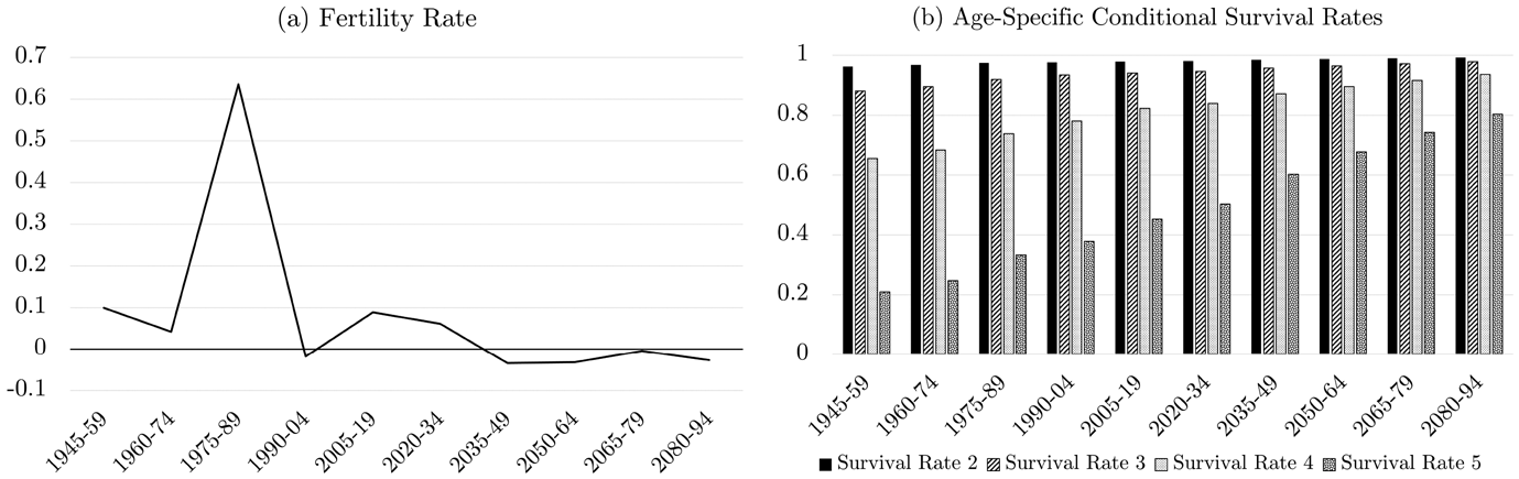
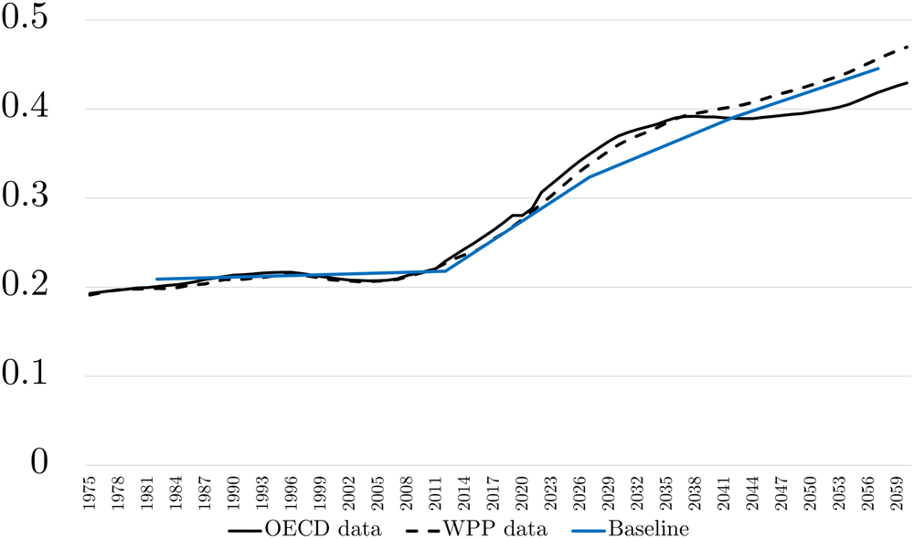
We simulate the deterministic model for the US using Dynare 4.6.4 (Adjemian et al., Reference Adjemian, Bastani, Juillard, Karamé, Maih, Mihoubi, Mutschler, Perendia, Pfeifer, Ratto and Villemot2011). Just as in Section 3.2, we impose exogenous paths for the five demographic parameters (one fertility rate and four survival rates), which are fully known beforehand by individuals in the model. These paths are shown in Figure 3 (more details in online Appendix C). Figure 4 shows that the resulting model old-age dependency ratio (size of the population aged at least 65 against the size of the population aged 20 to 64) matches the historical data and near-future projections well.
Path of exogenous demographic parameters for the US. The fertility rate in panel (a) refers to the growth rate of the size of the young generation in that period when compared to the size of the young generation in the previous period. The age-specific conditional survival rates in panel (b) refer to the probability that individuals of different age groups in the periods denoted on the horizontal axis survive into the next 15-year period of their lives. More detailed information can be found in online Appendix C.

Old-age dependency ratio in the US (65 + /20–64). The old-age dependency ratio refers to the ratio of the number of people who are at least 65 years old to the number of people aged 20 to 64. We compare the model's predictions under our baseline demographic scenario with the actual (projected) values. We take measures for the actual old-age dependency ratio based on (1) the OECD Historical Population Dataset and the OECD Population Projections, and (2) the United Nations Population Division's World Population Prospects (WPP).

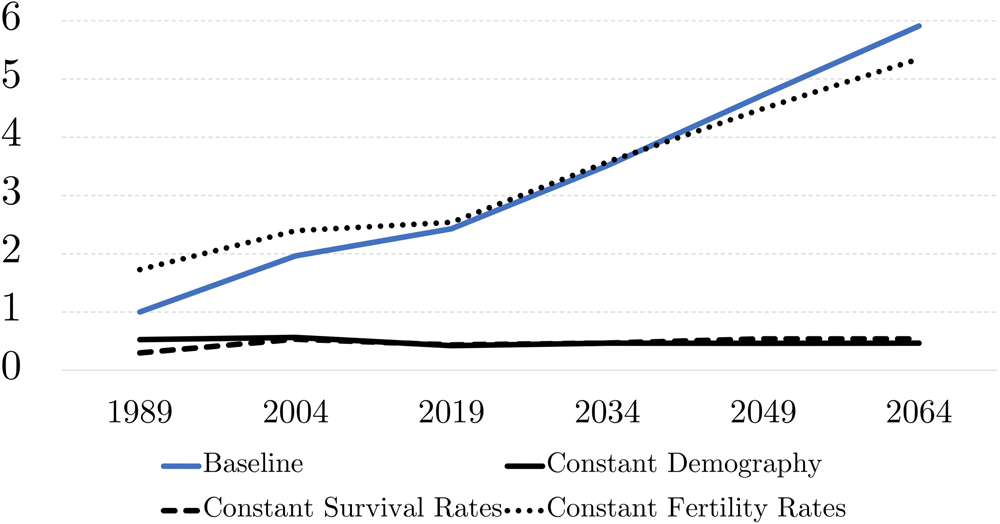
Figure 5 sets out how our measure of automation densityFootnote 12 varies over time under different demographic scenarios.Footnote 13 When comparing the baseline scenario with the “constant demography” case, it is immediately clear that demographic forces have induced a drastic increase in the take-up of automation technologies, and this is not projected to slow down in the near future. Even in the absence of any technical progress in automation technologies, our model generates a doubling of automation density over the past 30 years and it predicts another doubling over the next 30 years. Aging-induced automation is mostly driven by the large rise in life expectancy. If we shut down the impact of increased life expectancy, automation capital per worker remains almost constant. Changes in fertility appear to have contributed negatively to automation in the decades before 2019. The large pool of workers after the baby boom kept wages and incentives to automate relatively low. The retirement of the baby boomers and low fertility after the baby boom, turn fertility into a factor encouraging automation.
Evolution of automation capital per worker under different demographic scenarios13. “Automation capital per worker” refers to the ratio of the stock of automation capital at the end of the model period to the size of the workforce in that period. “Baseline” represents the realistic demographic scenario set out in Figure 3. “Constant survival rates” represents the case where all survival rates are kept at their 1945–59 level throughout the simulation. “Constant fertility” represents the case where model fertility rates are kept at zero throughout the simulation. “Constant demography” represents the combination of the latter two cases. All values are normalized such that automation density = 1 in 1989 under the baseline scenario.

4.1.2 The welfare effects of aging-induced automation
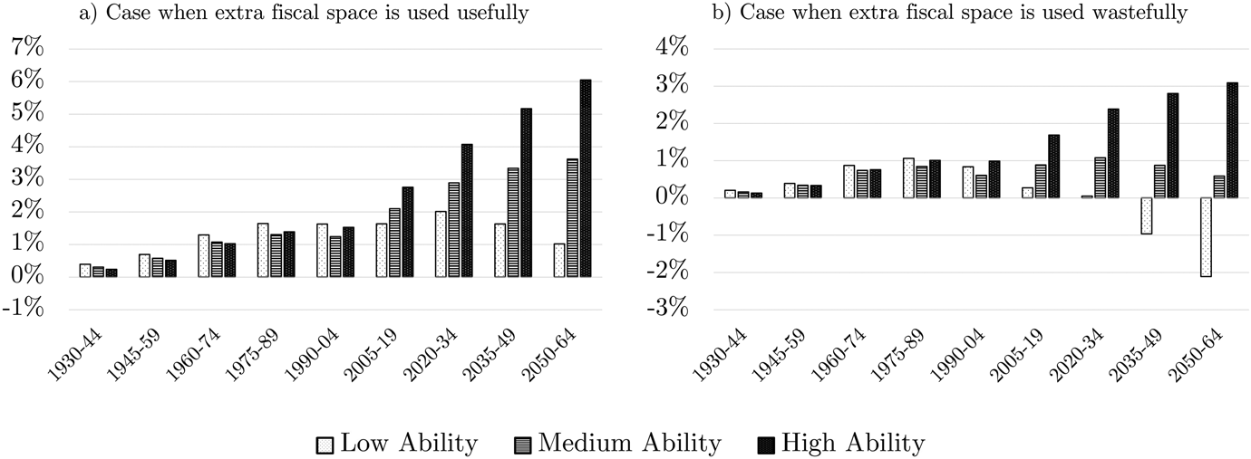
To evaluate the impact of the aging-induced automation, we compare the baseline results with the counterfactual scenario in which the level of automation capital per worker does not increase over time. More precisely, one could think of the counterfactual as representing the case where the use of automation technology is capped at the 1989 level (e.g., by policymakers). Since rational investors would want to invest more into automation technology, the no-arbitrage constraint can no longer hold and the return on automation capital exceeds that on traditional capital. The demographic conditions are identical in both scenarios, the only difference is whether or not aging is allowed to have its stimulative effect on automation. Comparing the discounted expected lifetime utility of each generation under both scenarios is then informative about the welfare effect of aging-induced automation. This is displayed in Figure 6 for consecutive generations. In the counterfactual scenario, we thus look at the consequences of aging when the incentive to automate is blocked (by regulation). This differs from the approach taken by Stähler (Reference Stähler2021) whose counterfactual looks at the consequences of aging in the absence of any automation technology. We argue that since aging directly impacts factor prices and not technology, our approach based on a scenario with counterfactual costs rather than counterfactual technology appears more suitable.
Welfare effect of aging-induced automation. The indicator considers the percentage increase in consumption in each remaining period of life that is necessary to raise an individual's expected lifetime utility under the constant automation density counterfactual to the expected lifetime utility level of an individual of the same generation t and same ability level a under the baseline scenario. Generations are identified by the period when they are young. That period is indicated on the horizontal axis. For example, panel a gives a value of around 4% for a high ability individual young in 2020–34. This implies that a high ability individual of that generation would require a 4% increase in consumption levels throughout their lifetime in the “constant automation” counterfactual to be equally well off in that scenario as under the baseline scenario with aging-induced automation.

Since allowing aging-induced automation helps the government cope with the budgetary impact of aging (cf. infra), we need to take a stand on how this additional fiscal space is used. In panel a, we adopt a more sanguine view on the role of public policymakers by assuming that the additional fiscal space is used usefully, i.e. to the direct benefit of individuals. In that case, the fiscal space will translate into more lump sum transfers (until 2005–19) and lower consumption taxes (from 2020–34 onwards). In panel b, we are more pessimistic about what policymakers do with the budgetary relief brought by aging-induced automation: it is solely used to increase wasteful government spending.
Regardless of the stance on public policy, it is clear that aging-induced automation has heterogeneous welfare effects across generations and ability. For older generations (1930–44 until 1990–04), the effects of aging-induced automation mostly take place when they have already retired. For them the welfare effects are small, positive, and relatively equal across ability types. For the younger generations (from 2005–19 onwards), the unequal wage effects of aging-induced automation during their working life dominate. We observe strong heterogeneity by ability type, with high ability individuals gaining much more than their low ability contemporaries. If the additional fiscal space generated by aging-induced automation is not usefully allocated, the welfare effects even turn negative for low ability individuals. They are then better off in the absence of aging-induced automation.
4.1.3 The macro effects of aging-induced automation
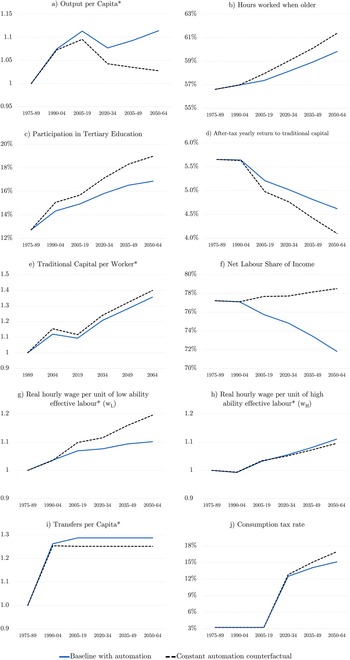
Figure 7 summarizes the dynamic simulation results of both the baseline with aging-induced automation and the counterfactual scenario where additional automation is capped at the 1989 level. Given our explanation above, the difference between the baseline and the counterfactual reveals the impact of the aging-induced automation. Based on panel (a), we conclude that the additional automation generated by demographic change has been a factor contributing to per capita growth in the past and it will be a factor softening the negative per capita output effect of rising old-age dependency in the future. We consider our results as evidence that is cautiously supportive of the hypothesis of Acemoglu and Restrepo (Reference Acemoglu and Restrepo2017). Automation largely neutralizes the negative effects of aging. By 2050–64, our baseline projection expects per capita output at the same level as the peak level of 2005–19. If aging-induced automation did not take place, per capita output would fall by more than 6% over the same period. Intuitively, when additional automation is allowed, the increased execution of automated tasks can compensate for the aging-driven shortage of human workers executing non-automated tasks. Automated and non-automated tasks are imperfect substitutes, however, such that the mitigation is only partial. Aging-induced automation cannot prevent that demographics weigh down per capita output in the next decades, as the baby boom generation retires.
Macro effects of aging-induced automation: simulation results for selected variables. Variables marked with an asterisk (*) are normalized to equal one in 1975–89, and they are detrended by the exogenous growth rate of technology x.

In panels (b) and (c), one can see the behavioral reactions to aging at play (Bloom et al., Reference Bloom, Canning and Fink2010). In line with the findings of Heijdra and Romp (Reference Heijdra and Romp2009) and Ludwig et al. (Reference Ludwig, Schelkle and Vogel2012), rising life expectancy stimulates investment in human capital considerably since individuals are more likely to be alive in stages of life where one can benefit from high human capital. The anticipation of a longer life as pensioner without labor income likewise leads individuals to work more when older (e.g., Devriendt and Heylen, Reference Devriendt and Heylen2020; Heijdra and Reijnders, Reference Heijdra and Reijnders2018). Crucially, one can observe that both behavioral effects are less strong when aging-induced automation takes place. The main driver of this result is the higher interest rate in this scenario (panel d). When the interest rate is higher, working when young and transferring income to the future through the accumulation of non-human wealth becomes more interesting relative to investing in the accumulation of human capital. Given the higher return on savings, individuals do not have to work as hard when older to achieve sufficient resources during retirement (income effect) and, given the lower amount of human capital, the financial return to work is also less worthwhile (substitution effect). This negative linkage between the automation reaction and the behavioral reaction to aging provides a second explanation for why the mitigation of aging-induced automation is incomplete in the near future.
In panel d, one can observe that demographic change is a factor drastically lowering the interest rate, consistent with earlier analyses of demographic change in an OLG context (Eggertsson et al., Reference Eggertsson, Mehrotra and Robbins2019; Gagnon et al., Reference Gagnon, Johannsen and Lopez-Salido2021; Ludwig et al., Reference Ludwig, Schelkle and Vogel2012). When the rise in automation capital is artificially suppressed by capping the level of automation, the fall in the interest rate is even more pronounced. Aging-induced automation thus partially counteracts the decline in the interest rate generated by demographic change. The main reason is that traditional capital and automation capital complement one another such that allowing investment in automation capital can help to keep the productivity of traditional capital high in times of rising capital intensity. It is also noteworthy that, when allowed, the rise in automation capital density is far more pronounced than the rise in traditional capital (Figures 5 and 7e). The intuitive explanation for this is that – because of its lower complementarity with human labor – automation capital thrives in an aging economy where labor is scarcer.
The strong aging-induced increase in the adoption of automation capital generates a fall in the labor share of income as firms substitute automated tasks for non-automated tasks (panel f). This reduces the gross labor share in our model since the elasticity of substitution between automated and non-automated tasks κ is higher than 1. It aligns our results with the findings of Bergholt et al. (Reference Bergholt, Furlanetto and Maffei-Faccioli2022), Dao et al. (Reference Dao, Das, Koczan and Lian2017), and Karabarbounis and Neiman (Reference Karabarbounis and Neiman2014), who regard automation as an important driver of the fall in the labor share. Rognlie (Reference Rognlie2014) points out that it is the net labor share that has distributional consequences for capital-owners and non-capital-owners. This clarifies the positive welfare effect in Figure 6 for older generations. Aging-induced automation mostly affects them when they are retired. Since they are only capital-owners then, not workers, they unambiguously gain when automation raises the return to capital and lowers the labor share. For the younger generations, aging-induced automation has unequal wage effects during their lifetime (results in panels g and h) hence the heterogeneity in the welfare effect. This aligns with some of the recent findings of Santini (Reference Santini2022) on the effect of automation on consumption inequality by education level.Footnote 14
Finally, panels (i) and (j) show the budgetary pressure that aging creates. To keep the public debt ratio constant in the face of a rising old-age dependency ratio, the government has to considerably raise consumption tax rates (panel j). If aging-induced automation is allowed to take place, the budgetary woes created by demographics are softened slightly: lump-sum transfers to the general public can be increased somewhat, and the consumption tax rate increase can be curbed. Panels (i) and (j) suppose that we adopt the sanguine view on public expenditure where the extra fiscal space is used to better the life of citizens. For low ability individuals of younger generations, the welfare effect of aging-induced automation is still positive under this scenario (though much smaller than for high ability individuals) (Figure 6a). The reason is that, although aging-induced automation lowers their wages (results in panels i and j), they are sufficiently compensated for this in terms of a higher interest rate, more transfers and a lower consumption tax rate. In the pessimistic scenario, panels (i) and (j) do not hold: the level of transfers per capita and consumption tax rate is then the same regardless of the automation scenario, with wasteful government consumption adjusting to absorb the fiscal benefits of aging-induced automation. In that scenario, low ability individuals are actually worse off under aging-induced automation as a result of their lower wages (Figure 6b).
4.2 Policy analysis
In section 4.1, we established how firms can mitigate the impact of the relative shortage of working-age individuals by making increased use of automation technologies. At the same time, however, the benefits of this induced automation are shared unequally. Depending on the way in which the additional fiscal space generated by automation is used, low ability individuals might stand to lose in absolute terms from the increased adoption of automation technologies. Frey (Reference Frey2019) argues that those harmed by the introduction of a new technology have the incentive to slow down its adoption or prevent it altogether. Whether or not the losers of technology adoption actually succeed in their efforts depends on the balance of political power, but as long as there is a sizeable group of individuals in society who are better off when technology adoption is halted, the risk of a so-called “technology trap” is present (Frey, Reference Frey2019). As a result, policymakers might wish to both (1) maximize the beneficial macro role of aging-induced automation, and (2) ensure a fairer distribution of the welfare gains related to aging-induced automation.
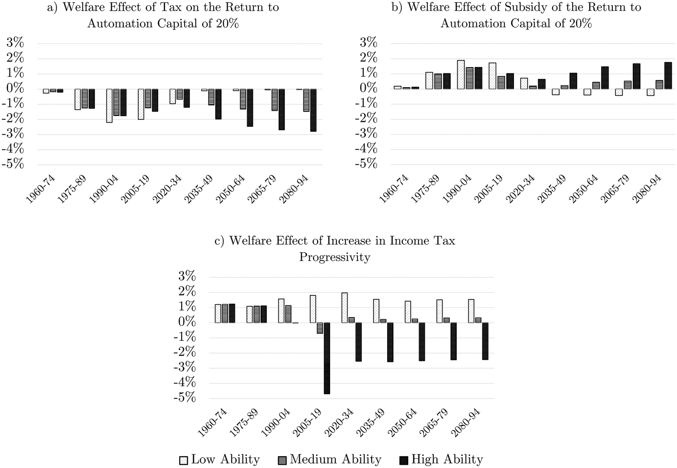
First, policymakers could consider either slowing down the adoption of automation technology by taxing its returns (thus making it a less enticing investment prospect), or further stimulating its adoption by subsidizing its returns. We consider the scenario where policymakers introduce a tax (subsidy) on the returns to automation capital of 20% from 2020–34 onwards. The reform is unanticipated such that the policy reforms have no effects before 2020. As in the baseline, the consumption tax rate adjusts endogenously to absorb the budgetary implications for the government. Figures 8(a) and (b) summarize the welfare effects of these reforms compared to the baseline, and Figure 9 summarizes its macro effects. In short, both reforms fail to deliver on the dual objective outlined above. Introducing an automation tax succeeds at countering the incentives to automation provided by aging and keeping up the labor share of income (Figure 9b and 9g), but it also negates the positive efficiency effects of such aging-induced automation (Figure 9a). As a result, an automation tax makes the welfare distribution fairer, but only through making everyone worse off (Figure 8a). A further subsidy to automation largely has the opposite consequences, thus succeeding at the condition of macro efficiency, but only by making the unequal welfare effects of aging-induced automation even more pronounced.
Welfare effect of policy reforms. The indicator considers the percentage increase in consumption in each remaining period of life that is necessary to raise an individual's expected lifetime utility under the baseline scenario with aging-induced automation to the expected lifetime utility level of an individual of the same generation t and same ability level a under the policy reform scenario. Generations are identified by the period when they are young. That period is indicated on the horizontal axis. For example, panel a gives a value of around −2% for a high ability individual young in 2035–49. This implies that, for a high ability individual of that generation, the introduction of the automation tax affects lifetime utility in the same way as a 2% decrease in consumption levels throughout their lifetime.

Macro effects of policy reforms: simulation results for selected variables. Variables marked with an asterisk (*) are normalized to equal one in 2005–19, and they are detrended by the exogenous growth rate of technology x.

A second possibility consists of countering the rise in income and welfare inequality brought about by automation by raising the progressivity of the income tax system. We consider the scenario where the progressivity parameter ψ of the US income tax system is raised by 50% from 2020–34 onwards, thus increasing from 0.48 to 0.72. Again, the reform is unanticipated such that it has no effects before 2020 and the consumption tax rate adjusts to absorb the budgetary implications for the government. The welfare effects, described in Figure 8(c), indicate that a progressive income tax reform is to be preferred above an automation tax. While an automation tax throws away the baby with the bathwater (only redistributing welfare by reverting the macro benefits of aging-induced automation), the progressive income tax reform redistributes the gains of aging-induced automation without undoing it. A progressive income tax even slight stimulates the adoption of automation technologies (Figure 9b), because the redistribution towards low ability individuals implies more savings (since these cannot rely on higher education for transferring income into the future and thus start saving for retirement earlier in their lifespan). That is not to say that rising income tax progressivity is without efficiency costs: higher marginal tax rates dissuade people from participating in the labor market when older and from investing in human capital (Figure 9c and 9d) thus lowering output per capita (Figure 9a). The efficiency costs are far smaller than those of blocking automation altogether, however. There seems to be a case for the combined policy package of (1) allowing (or even stimulating) the adoption of automation technologies to counteract the labor scarcity in times of aging, and (2) ex post remediating the higher market inequalities generated by automation through the income tax system. A clear promise on this ex-post redistribution can help to pave the way for the adoption of automation technologies by making them less controversial (Frey, Reference Frey2019). In the absence of such redistribution, lack of public support for its adoption might a suboptimal scenario where automation is dissuaded in the first place (Figure 8a).
5. Conclusion
In this study, we constructed and calibrated an overlapping generations model with the aim to re-evaluate the macro effects of aging in a context where firms can respond to population aging by automating the production process. We test the hypothesis that the aging-induced adoption of automation technologies may compensate for the negative per capita output effect of aging. We paid special attention to the theoretical and empirical foundations of the modeling of automation. Theoretically, we innovate by integrating the notion of two capital types into the task-based approach to automation. Empirically, we tested the validity of our approach by comparing model predictions of automation density to actual data on robotization in a cross-country fashion. Another important contribution to the automation literature is that we examine how automation interacts with behavioral adjustments to aging (employment at older age and human capital investment) which also counteract labor scarcity. The recent literature on aging and automation (e.g., Basso and Jimeno, Reference Basso and Jimeno2021; Irmen, Reference Irmen2021; Stähler, Reference Stähler2021; Zhang et al., Reference Zhang, Palivos and Liu2022) has largely neglected empirical validation and the role of behavioral adjustments to aging.
Our main findings are as follows. Aging strongly stimulates the adoption of automation technology and, in the long run, the negative growth effect of aging can largely be undone by this aging-induced automation. In the absence of further technical progress in automation technologies, however, demographic change will still constitute a force weighing down per capita output in the next few decades. Likewise, the fall in the interest rate that aging induces, is softened by aging-induced automation, but not halted. One reason for why aging still affects growth negatively is that automated tasks are far from perfect substitutes for tasks executed by human labor. A second reason is that, as aging-induced automation softens the relative shortage of human labor generated by aging, it also reduces the strength of the behavioral reactions to aging. Without aging-induced automation, the incentive to retire later and invest more in human capital accumulation would be stronger. Moreover, the partial mitigation also comes at the cost of heightened inequalities. First, aging-induced automation generates a fall in the labor share of income. Second, it also increases welfare inequality between workers with different ability. To remediate these inequalities, we find that progressively redistributing ex post yields better results than stopping automation in its tracks.
For these same two reasons, we conclude that the findings of several recent studies (e.g., Irmen, Reference Irmen2021; Zhang et al., Reference Zhang, Palivos and Liu2022) regarding the mitigating role of automation in times of aging may be too optimistic. An important limitation of this study is its focus on the effects of aging on the adoption of existing automation technologies. Aging might in reality also stimulate R&D in automation technology and thus foster technical change. A more optimistic interpretation of the results therefore readily presents itself: even without technical progress, the automation technologies of today can considerably soften the negative macro effects of aging.
Supplementary material
The supplementary material for this article can be found at https://doi.org/10.1017/dem.2024.10.
Funding statement
Arthur Jacobs is the recipient of a PhD Fellowship grant from the Research Foundation Flanders (Grant Number: 1115623N). He also thanks the National Bank of Belgium (NBB) for financial support via UGent BOF. The author has no other relevant financial or non-financial interests to disclose.
Competing interests
None.
Author contributions
All authors contributed to the study conception and design. Data collection and analysis were performed by Arthur Jacobs. The first draft of the manuscript was written by both Arthur Jacobs and Freddy Heylen and all authors commented on previous versions of the manuscript. All authors read and approved the final manuscript.
Appendix A
Task-based framework of automation
Part 1 – Derivation of the necessary condition that has to hold such that all automatable tasks are fully automated
We start out from the most general expression for H L,tot,t (in equation 7a) and we set the productivity λ of human labor at the execution of automatable tasks (relative to its productivity at the execution of non-automated tasks) at 1/3.Footnote 15 The total execution of tasks of the low ability type H L,tot,t can then be written as:

Given that the productivity of low ability human labor at the execution of tasks depends only on whether or not the task is automatable, the amount of low ability labor assigned to any low ability task will not depend on the index i of the task but only on whether the task is automatable or non-automatable. We define l L,2,t as the human labor devoted to the execution of any automatable task t L,k,t of the low ability type (with k > ξ L) at time t. Correspondingly, l L,1,t is the human labor devoted to the execution of any non-automatable task t L,k,t of the low ability type (with k < ξ L) at time t.

Deriving Y t with regard to l L,2,t results in:

Deriving Y t with regard to P t results in:

when applying the Leibniz integral rule for definite integrals with constant lower and upper limits, we get:


As a result we obtain the following expressions for ∂Y t/∂l L,2,t and ∂Y t/∂P t:


We now proceed by evaluating the ratio (∂Y t/∂P t)/(∂Y t/∂l L,2,t) for l L,2,t = 0 and we verify that this ratio is, – throughout our simulations – larger than ([r t (1 − τ p)−1 + δ p]/(1 − ξ a)w L,t) (being the cost of capital relative to the cost of human labor)Footnote 16. Note that evaluating this inequality for l L,2,t = 0 is sufficient since the ratio (∂Y t/∂P t)/(∂Y t/∂l L,2,t) will be the lowest for l L,2,t = 0. This is the case because any increase in l L,2,t would leave the ratio (∂H L,tot,t/∂P t)/(∂H L,tot,t/∂l L,2,t) unchanged (at a constant value of 3j), but it would increase the productivity of automation capital in the execution of tasks of ability types different from L by increasing H t (in the second term of expression A8). As such, if the inequality holds for l L,2,t = 0, it also holds for higher values of l L,2,t.
When evaluating (∂Y t/∂l L,2,t) for l L,2,t = 0, we find:

And since J = j ((κ−1)/κ)

When evaluating ∂Y t/∂P t for l L,2,t = 0, we find:

And since J = j ((κ−1)/κ)

We find that, given our parameterization, the following inequality holds throughout all of our simulations for any country:

Mutatis mutandis, the same inequality holds true for medium and high ability tasks. As a result, it is strictly cheaper for firms to use automation capital for the execution of automatable tasks of any ability type: no human labor is assigned to execute automatable tasks $( l_{a, i, t} = 0\;\;\forall i > \xi _{a, \;\;}\;\forall a = L, \;M, \;H)$ .
Part 2 – Proof of the validity of equation (7b)
Our starting point is the expression for H a,tot,t defined in equation (7a):

with

and


Given our calibration, it is at any point cost-effective for firms to only use automation capital to execute automatable tasks (see Part 1 of this Appendix A). We can therefore state that:


Given that the productivity of human labor at the execution of any task i < ξ a is identical, the same amount of human labor will be used for any task of type a with index i < ξ a such that l a,i,t = l a,t (A16) holds.

The total amount of human labor provided by individuals of a particular ability level H a,t is allocated over the different non-automated tasks of type a such that:


This final expression results in equation (7b) of the main text.
Appendix B
Evaluating the sign of mixed second order derivates: q-substitutability?
The real hourly wage per unit of human labor of individuals of ability type a equals the marginal product of effective human labor of type a. The equation below is equation (11) in the main text.

After rearranging, a non-negative expression E t, that is independent of P t, can be put in front.

This simplified expression for the real wage per unit of human capital is now derived with respect to the stock of automation capital P t.

After rearranging, a non-negative expression F t, that is independent of P t, can be put in front.

The non-negative expressions E t and F t are not relevant when determining the sign of the expression:

Based on this final expression, we can draw conclusions with regard to why the effects of an increase in automation capital vary over the different ability types. For this interpretation, we refer to sub-section 3.1.6 of the main text.