A. Si-face graphene

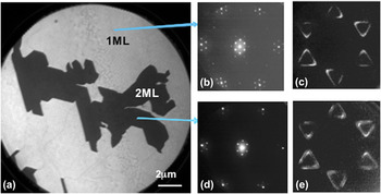
For comparison between graphene grown on C-face and Si-face SiC, some selected results ^{Reference Zakharov, Virojanadara, Watcharinyanon, Yakimova and Johansson36} from a Si-face sample are shown in Fig. 1. This is a 1-ML graphene sample with 2-ML islands on it, and a typical LEEM image is shown in Fig. 1(a). Based on the observed variation ^{Reference Hibino, Kagashima, Maeda, Nagase, Kobayashi and Yamaguchi37} in the electron reflectivity with electron energy, one can immediately determine that the islands in the LEEM image correspond to 2 MLs and the brighter areas to 1-ML graphene. The field of view (FOV) in Fig. 1(a) is 20 μm. It deserves to be noted that Si-face samples where a homogenous coverage of 1-ML graphene is observed in LEEM images recorded at an FOV of 50 μm have been possible to prepare. ^{Reference Virojanadara, Yakimova, Osiecki, Syväjärvi, Uhrberg, Johansson and Zakharov7} The selected area LEED diffraction patterns originating from the 1- and 2-ML areas in Figs. 1(b) and 1(c), respectively, show a distinct decrease in spot intensities around the main graphene spots for the 2-ML island. These additional spots originate from the first carbon layer formed on Si-face SiC, the 6√3 × 6√3R30° reconstructed buffer layer; so these patterns show that diffracted intensity is observed from at least three carbon layers at this electron energy. Diffraction patterns from different 1- and 2-ML areas look essentially identical all over the sample, only some variation in relative intensity between buffer layer spots is observed. ^{Reference Virojanadara, Yakimova, Osiecki, Syväjärvi, Uhrberg, Johansson and Zakharov7} The buffer layer forms strong covalent bonds to the SiC substrate. It does not exhibit the electronic properties of graphene, i.e., shows no graphene π-band at the $\bar K$ point ^{Reference Emtsev, Speck, Seyller, Ley and Riley19} and gives rise to an additional shifted component ^{Reference Emtsev, Speck, Seyller, Ley and Riley19,Reference Johansson, Owman and Mårtensson38} in the C 1s core level spectrum. Selected area constant initial energy PAD patterns recorded ^{Reference Zakharov, Virojanadara, Watcharinyanon, Yakimova and Johansson36} from the 1-ML or the 2-ML areas, respectively, are shown in Figs. 1(d) and 1(e). They were collected from a small (800 nm) area using XPEEM, a photon energy of 35 eV, and at an energy of 2.5 eV below the Fermi level. The six Dirac cones in the Brillouin zone are clearly revealed and seen to have a triangular shape at this energy of approximately 2 eV below the Dirac point. From the 2-ML island, the second π-band cone becomes clearly observable, see Fig. 1(e), in this data set that was taken at the highest possible instrument energy resolution (∼0.15 eV). When using photons in this energy range, contribution from three to four graphene layers can ^{Reference Ohta, Bostwick, McChesney, Seyller, Horn and Rotenberg22} typically be distinguished. For the graphene forming on the Si-face, a single π-band (cone) with linear dispersion at the $\bar K$ point results ^{Reference Latil, Meunier and Henrard39} only for single layer graphene, whereas bi- and trilayer graphene show ^{Reference Latil, Meunier and Henrard39,Reference Latil and Henrard40} two and three split parabolic π-bands (cones) at the $\bar K$ point, respectively. If the two layers on the 2-ML islands instead would be decoupled, i.e., behave as independent single layers of graphene as suggested for multilayer C-face graphene, and moreover be rotated azimuthally relative to each other by an angle different than 60° × integer, one would in Fig. 1(e) see two sets of these six Dirac cones rotated relative to each other by exactly that angle. In selected area LEED, not only two rotated (1 × 1) patterns would then be seen but also characteristic additional diffraction spots, originating from the sum and difference between the two sets of reciprocal lattice vectors, would appear. ^{Reference Ohta, Beechem, Robinson and Kellogg41} Thus, both in selected area LEED patterns and selected area PAD images, it is possible to directly reveal if adjacent graphene layers are rotationally disordered, i.e., if they are rotated azimuthally relative to each other by an angle different than 60° × integer.

FIG. 1.

(a) LEEM image collected from a furnace-grown 6H-SiC Si-face graphene sample at an FOV of 20 μm and an electron energy of 4.6eV. Micro-LEED patterns (400-nm probing area) recorded at 60 eV from (b) 1-ML and (c) 2-ML areas. High energy resolution PADs, E _i(k _x ,k _y ), collected from (d) 1-ML and (e) 2-ML graphene areas at an initial energy, E _i, of 2.5 eV. Two π bands are clearly seen from the 2-ML areas.

B. C-face graphene

Results from three different C-face graphene samples, all grown at high sublimation temperature and in an Ar ambient, are presented for the purpose to illustrate typical results concerning surface morphology, structure, and stacking and differences compared to Si-face samples. A LEEM image collected from one 6H-SiC C-face graphene sample at an electron energy of 3.3 eV and an FOV of 10 μm is shown in Fig. 2(a). The electron reflectivity versus electron kinetic energy curve, i.e., the so-called I(V) curve, extracted from the areas labeled from A to P are shown in Fig. 2(b). Curves A to I are very similar and show two pronounced minima that indicate 2-ML graphene. Curves J to N also show two minima indicating a coverage of 2 MLs, although these curves have a slightly different shape around 2 eV than curves A to I. Curve O shows one dip indicating monolayer graphene, and curve P represents an area with no graphene coverage. Most of the surface of this sample has a graphene coverage of 2 MLs. Selected area LEED patterns collected from areas E and D at an energy of 45 eV are shown in Fig. 2(c). A probing area with a diameter of 0.4 μm was used, so that both patterns are collected from a single grain/domain, and the two domains are seen to have different azimuthal orientations. C 1s spectra collected, using conventional macro-PES, from this “2-ML” graphene sample at three photon energies are shown in Fig. 2(d). They are modeled accurately using only two components, the SiC component from the substrate and the G component from the graphene layers. In agreement with earlier results, ^{Reference Johansson, Watcharinyanon, Zakharov, Iakimov, Yakimova and Virojanadara11,Reference Emtsev, Speck, Seyller, Ley and Riley19} no trace of a carbon buffer layer component can be observed. The energy separation of 1.9 eV and peak intensity ratio of around 6 (at 600 eV) determined between the graphene and the SiC components (G/SiC) are consistent with previously determined values ^{Reference Emtsev, Speck, Seyller, Ley and Riley19} for a graphene thickness of about 2 MLs. The π-band recorded, using conventional macro-ARPES, from this 2-ML graphene sample around the $\bar K$ point and along the A– $\bar K$ –A′ direction using a photon energy of 33 eV is shown in Fig. 2(e). The Dirac point is located within approximately 75 meV below the Fermi level indicating a slight n-doping instead of the slight p-doping earlier reported. ^{Reference Siegel, Hwang, Fedorov and Lanzara34} Since the graphene grain size was only on the order of a few micrometers, a few π-cones from domains of different azimuthal orientations were typically detected when moving the light spot over the sample. However, the Dirac point of the different cones appeared always located at the same energy position.

FIG. 2.

(a) LEEM image recorded from a 6H-SiC C-face graphene sample at 0.4 eV and an FOV of 10 μm. (b) I(V) curves extracted from the different areas labeled A to P in (a), showing a coverage of mainly 2 MLs of graphene. (c) Micro-LEED patterns, collected at 45 eV using a probing area diameter of 400 nm, from two different grains/domains in (a). (d) C 1s spectrum recorded using three different photon energies showing contribution from graphene (G) and the SiC substrate. (e) The π-band recorded around the $\bar K$ point using a photon energy of 33 eV.

An LEEM image collected from a 4H-SiC C-face sample at 1.3 eV and an FOV of 10 μm is shown in Fig. 3(a). The extracted reflectivity curves from the areas labeled 1–8, respectively, in Fig. 3(b) show that several of them have the same number of graphene layers. Six minima are clearly observed in curves 1, 2, 6, 7, and 8, whereas curves 3, 4, and 5 at first appear to have only five minima. However, when looking in detail at these latter three curves, one finds that there actually appears a weak minimum at around 6.5 eV. The coverage may be 6 MLs over the whole area in Fig. 3(a), but if some areas actually have 5 MLs is not important for the main message contained in Figs. 3(c) and 3(d). The selected area LEED patterns collected using a probing area of 400 nm from the positions labeled 1 and 2 in Fig. 3(a) are shown in the two upper panels in Fig. 3(c). It is obvious from these LEED patterns that a grain size larger than 400 nm has been accomplished on this sample and that the stacking of the six graphene layers is such that adjacent layers are not rotated with respect to each other. The third, bottom, panel in Fig. 3(c) shows the LEED pattern collected using a 5-μm large probing area at position 2. The sampled area then includes domains 2 and 1, and it is obvious that two grains of different azimuthal orientations are now probed since this LEED pattern just represents a superposition of the patterns shown in the upper two panels. The characteristic additional diffraction spots, ^{Reference Ohta, Beechem, Robinson and Kellogg41} originating from rotated/twisted layers are not discernable. To further emphasize that grains of six layers of graphene can form on the C-face and be stacked in such a way that no rotational disorder exists between adjacent layers, some PADs of the π-band were also recorded. Two such patterns collected using a probing area of 800 nm, a photon energy of 45 eV, and at an energy of about 2 eV below the Fermi energy are shown in Fig. 3(d). Only six Dirac cones, which appear triangular at this initial energy centered around the six $\bar K$ points in the Brillouin zone are observed in these patterns. They were collected at two different locations outside the area shown in Fig. 3(a) but where the number of graphene layers was also six. These patterns show clearly that well ordered grains of multilayer graphene larger than 800 nm has formed and that adjacent graphene layers are not rotated relative to each other. At this photon energy, separate and distinguishable signals from three to four layers of graphene have been demonstrated from Si-face samples. ^{Reference Ohta, Bostwick, McChesney, Seyller, Horn and Rotenberg22} Moreover, the PAD patterns recorded ^{Reference Zakharov, Virojanadara, Watcharinyanon, Yakimova and Johansson36} from bilayer graphene show two π-cones of fairly similar intensity centered around each $\bar K$ point so any rotational disorder present between the two and three uppermost graphene layers would show up directly in these patterns. The two patterns, in Fig. 3(d), show that the different grains probed do have different azimuthal orientations. It should be noted that when selecting a larger probing area that included two grains of different azimuthal orientations, two sets of superimposed Dirac cones were detectable, just similar to the two superimposed micro-LEED patterns shown in the bottom panel in Fig. 3(c).

FIG. 3.

(a) LEEM image recorded from a 4H-SiC C-face graphene sample at 1.3 eV and an FOV of 10 μm. (b) Electron reflectivity curves extracted from different areas labeled 1–8. (c) The two upper panels show selected area LEED patterns collected at 45 eV using a probing area of 400 nm from the positions labeled 1 and 2 in Fig. 3(a). The lower panel shows the LEED pattern collected using a 5-μm aperture at position 2. (d) Shows two constant initial energy PAD patterns, E _i(k _x ,k _y ), of the π-band collected using a probing area of 800 nm, a photon energy of 45 eV, and at an energy of about 2 eV below the Fermi level. One Dirac cone centered around each of the six $\bar K$ points in the Brillouin zone is clearly observed.

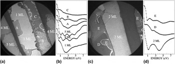
Two LEEM images from different locations of another C-face graphene sample are shown in Figs. 4(a) and 4(c). These images were collected at an FOV of 25 μm and energies of 3.9 and 5.1 eV, respectively. Several different domains are clearly visible, and the I(V) curves extracted from the different domains, displayed in Figs. 4(b) and 4(d), show the number of graphene layers present. The lightest gray areas in Fig. 4(a) have a graphene coverage of 1 ML, whereas some other areas have thicknesses of 4 MLs and 5 MLs of graphene. In Fig. 4(c), the light gray areas have a coverage of 2 MLs. The other I(V) curves, labeled A, B, C, D, and E, do not show similarly well-defined modulations in the reflectivity and indicate areas where a mixture of different numbers of graphene layers probably exist. The really dark areas in both Figs. 4(a) and 4(c) showed no graphene coverage but the presence of an ordered silicate, observed and discussed earlier. 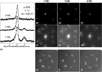^{Reference Luxmi, Srivastava, He, Feenstra and Fisher9–Reference Hicks, Shepperd, Wang and Conrad13} However, the important point here is that large enough areas of 1 ML, 2 MLs, and 4 MLs of graphene were identified by LEEM, so selected area PES, LEED, and XPEEM could be applied. Selected area C 1s spectra collected using a photon energy of 450 eV and a probing area of 4 μm are displayed in Fig. 5(a). Contribution from the SiC substrate is clearly resolved, at around 1.9 eV lower binding energy than the graphene component, in the spectra from the 1-ML and 2-ML areas but is not discernible from areas having 4-ML graphene. These C 1s spectra show no hint of a dense disordered carbon interface layer, which earlier has been proposed to be present, at least locally. ^{Reference Mathieu, Barrett, Rault, Mi, Zhang, de Heer, Berger, Conrad and Renault10,Reference Hicks, Shepperd, Wang and Conrad13} Selected area LEED patterns collected using two different electron energies from the three areas with different graphene coverage are shown in Figs. 5(b)–5(g). A probing area of 1.5 μm was utilized, so the pattern is in each case collected from a single crystallographic grain having a specific number of graphene layers. The patterns collected at 45 eV, Figs. 5(b), 5(d), and 5(f), all show distinct (1 × 1) patterns and no presence of additional superstructure spots. When increasing the energy to 145 eV, additional weaker spots, of which three are marked by white circles, are possible to be observed in the patterns from the 1-ML and 2-ML areas, whereas such spots are not visible in the pattern from the 4-ML area. These weaker spots are interpreted to originate from the SiC substrate, since the (1 × 1) diffraction spots from the SiC substrate and graphene appear at the same distances, within the experimental uncertainty, for graphene grown on Si-face SiC, as can be seen in Fig. 1(b). There, the substrate spots are always rotated 30° relative to the graphene (1 × 1) spots, and although the angle is close to 30°, also in this case, we observed at other locations and for other samples a different angle. No additional superstructure spots originating from rotated graphene layers are thus observed in any of the micro-LEED patterns in Fig. 5. To further demonstrate that the graphene layers are stacked in such a way that no rotational disorder exists between adjacent layers, recorded PADs of the π-band from areas with a different numbers of graphene layers are shown in Figs. 5(h)–5(j). These patterns were collected using a probing area of 800 nm, a photon energy of 45 eV, and at an energy of about 1.5 eV below the Fermi energy. Only six Dirac cones, centered around the six $\bar K$ points in the Brillouin zone are observed. The patterns thus show clearly that well-ordered grains of multilayer graphene larger than 800 nm have formed and that adjacent graphene layers within these grains are not rotated relative to each other.

FIG. 4.

LEEM images collected at an FOV of 25 μm from a 6H-SiC C-face graphene sample using an energy of (a) 3.9 eV and from another position (c) at an energy of 5.1 eV. The I(V) curves in (b) and (d), extracted from different locations in (a) and (c) respectively, reveal fairly large areas of 1, 4, and 5 MLs and 2 MLs of graphene.

FIG. 5.

(a) C 1s spectra collected, using a probing area of 4 μm, from the marked areas in Fig. 4 with different numbers of graphene layers. (b)–(g) show 1.5-μm selected area LEED patterns from: the 1-ML area at (b) 45 eV and (c) 145 eV; the 2-ML area at (d) 45 eV and (e) 145 eV; and the 4-ML area at (f) 45 eV and (g) 130 eV, respectively. In (h)–(j), PADs, E _i(k _x ,k _y ), recorded from, respectively, the 1-ML, 2-ML, and 4-ML areas are shown. The PADs were collected at 1.5 eV below the Fermi level, using a probing area of 800 nm.

C. Hydrogen-treated C-face graphene

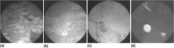
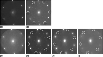
Intercalation of hydrogen of Si-face graphene has been quite thoroughly studied, ^{Reference Starke, Forti, Emtsev and Coletti8,Reference Riedl, Coletti, Iwasaki, Zakharov and Starke23–Reference Watcharinyanon, Virojanadara, Osiecki, Zakharov, Yakimova, Uhrberg and Johansson25} but no investigation of hydrogen intercalation of C-face graphene had been reported. Therefore, a receipt earlier successfully applied ^{Reference Ul Hassan, Virojanadara, Meyer, Ivanov, Flege, Watcharinyanon, Falta, Johansson and Janzén42} to intercalate hydrogen on Si-face graphene samples was utilized, i.e., heating in a pure hydrogen ambient at 700 °C, to treat C-face graphene samples and study the effects. A LEEM image, collected at 1.7 eV and an FOV of 50 μm, from a C-face sample grown by sublimation at a high temperature in an argon atmosphere, is shown in Fig. 6(a). It is a representative image of the surface morphology, since similar images were obtained at other positions on this sample. After hydrogen treatment, the LEEM images obtained were distinctly different, as illustrated by the representative image in Fig. 6(b). The domain structure clearly observed on the as-grown sample has more or less disappeared after hydrogen treatment, and considerably smaller domains and contrast variations are observed. For the as-grown sample, in Fig. 6(a), I(V) curves showing pronounced periodic variations indicating a coverage of mainly 3 and 4 MLs of graphene were extracted. For the hydrogen-treated sample, Fig. 6(b), extracted I(V) curves also showed periodic variations but considerably less pronounced. Selected area LEED patterns collected appeared clear and distinct but were found to change with time when using the typical micro-LEED electron beam current of 200 nA. The beam actually produced changes on the surface that were clearly detectable by LEEM after only a few minute exposure, as illustrated in Figs. 6(c) and 6(d). This hydrogen-treated sample was initially grown by sublimation at a lower temperature and in high vacuum and can then be expected to initially have smaller graphene grains/domains. For Si-face graphene, it is well known that sublimation growth at lower temperatures and in high vacuum result in significantly smaller domains than at high temperature and in an Ar ambient. With more grain boundaries and thus defects present on the surface, the effects of hydrogen exposures can be expected to be larger. This sample was deliberately exposed to the typical micro-LEED electron beam current over an area with a radius of approximately 5 μm for about 2 min. The illuminated circular area appears darker and brighter in the LEEM images in Figs. 6(c) and 6(d) that were collected at an FOV of 25 μm and energies of 1.7 and 6.5 eV, respectively. This clearly demonstrates that the typical micro-LEED electron beam current does induce changes in hydrogen-treated C-face graphene samples, and hydrogen desorption appears to be the most likely reason. Before looking at how the micro-LEED pattern typically changed with time, it deserves to be mentioned that for this hydrogenated sample, in Figs. 6(c) and 6(d), the I(V) curves extracted outside the illuminated circular area did not show any periodic oscillations, but instead appeared similar to curve C in Fig. 4(b), irrespective of the size and position of the area selected. For this sample, the hydrogen treatment thus drastically affected the size of the domains and apparently also perturbed the periodicity in distance between the graphene sheets, since no interference effect was possible to observe in extracted reflectivity curves. Distinct changes in the micro-LEED pattern appeared rapidly, however. The pattern in Fig. 7(b) was recorded 2 min after that in Fig. 7(a) from the same spot of the hydrogen-treated sample. An energy of 45 eV and a probing area of 1.5 μm was selected, and this sample was the one initially prepared at low sublimation temperature and in high vacuum. The superstructure spots become clearly visible after only about 1 min of electron beam exposure. The strongest of the superstructure spots are marked by white circles in Fig. 7(b), and they are seen to have the same distance to the (0, 0) spot as the initial (1 × 1) graphene spots. In addition to these strong spots, there are other spots arranged in inner hexagonal patterns, like in the patterns recently reported ^{Reference Ohta, Beechem, Robinson and Kellogg41} for specially prepared twisted bilayer graphene samples. When decreasing the micro-LEED electron beam current, to 10 nA, and moving to another spot on the sample, the pattern in Fig. 7(c) was obtained, which again is mainly a (1 × 1) graphene pattern. When increasing the electron beam current again, to 200 nA, the pattern in Fig. 7(d) resulted, which shows a similar set of six strong superstructure spots, although now at a different rotation angle. When increasing the electron energy to 80 and 142 eV, the same pattern remained, see Figs. 7(e) and 7(f); only the relative intensity between the main and superstructure spots is changed. These superstructure spots can be explained in the same way as earlier proposed ^{Reference Ohta, Beechem, Robinson and Kellogg41} for twisted bilayer graphene samples, indicating a twist angle of around 35 and 20° in Figs. 7(b) and 7(d), respectively. Since this effect with electron beam exposure did not occur for the as-prepared graphene C-face samples, desorption of intercalated hydrogen appears as the most plausible explanation. Moreover, after local hydrogen desorption by electron beam illumination, the two uppermost graphene layers appear in general to be twisted relative to each other, which definitely was not the case on the large ordered grains on the as-prepared samples [see Figs. 2(c), 3(c), and 5(b)–5(g)]. Therefore, the hydrogen-treated sample was also heated in situ at 600 °C for a couple of minutes in an effort to desorb most of the hydrogen. The micro-LEED patterns collected afterward using the normal typical high electron current then showed no time effect. Stable (1 × 1) patterns, and also patterns containing superstructure spots similar to those in Fig. 7, were then obtained at different positions on the surface. However, extracted I(V) curves still did not show pronounced periodic variations; they still appeared similar to curve C in Fig. 4(b), irrespective of the size and position of the area selected. Before heating, selected area PES core level spectra were collected from the hydrogen-treated samples, both from areas previously illuminated and not illuminated by the LEED electron beam. No difference in the chemical composition between these areas could be revealed by the core-level spectra, which suggests local hydrogen desorption as the probable origin to the changes observed in the LEEM images in Figs. 7(c) and 7(d). A hydrogen treatment, which for Si-face graphene results in intercalation and improved properties, for C-face graphene instead results in deteriorated properties. The average grain/domain size is drastically reduced; adjacent graphene layers appeared for one sample to become decoupled, since no clear interference effect was observable in extracted I(V) curves, and after local hydrogen desorption by the electron beam, adjacent graphene layers are in general rotated relative to each other. Heat treatment of a hydrogenated C-face graphene sample did not restore the quality of the original as-grown sample; considerably smaller domain/grain sizes showing either (1 × 1) or twisted layer micro-LEED patterns were then observed. Thus, the hydrogen treatment tried for the C-face graphene samples had, contrary to the case for Si-face graphene, a detrimental effect on the quality and properties of the graphene.

FIG. 6.

LEEM images collected from a 6H-SiC C-face graphene sample at 1.7 eV and an FOV of 50 μm: (a) as-grown and (b) after hydrogen treatment. The images in (c) and (d) were collected at an FOV of 25 μm from another hydrogen-treated sample at energies of 1.7 and 6.5 eV, respectively. The circular dark and bright spot seen in (c) and (d) was created by electron beam illumination during collection of micro-LEED patterns.

FIG. 7.

(a) to (d) micro-LEED patterns recorded, from the hydrogenated sample shown in Figs. 6(c) and 6(d), using an energy of 45 eV and a probing area of 1.5 μm. The pattern was found to change from the (1 × 1) in (a) to that in (b), containing superstructure spots within a minute. When moving to another spot on the sample and using a low electron beam current, the (1 × 1) pattern in (c) was observed. When increasing to the normally used high electron beam current, the pattern in (d) appeared within a minute. The same pattern collected at (e) 80 eV and (f) 142 eV.

D. Effects induced in the π-band structure by deposited sodium

The effects induced in the π-band structure close to the $\bar K$ point, after Na deposition and subsequent heating, were investigated ^{Reference Johansson, Xia and Virojanadara35} using conventional ARPES, on a C-face sample having predominantly 2-ML graphene coverage, actually the one presented in Fig. 2. After Na deposition, the Dirac point shifts down by about 0.5 eV, as shown in Fig. 8. Subsequent heating at 50 and 80 °C do not affect the band much, it only appears slightly more diffuse. Heating at temperatures from 120 to 300 °C results in a considerable broadening of the spectral features. At 400 °C, the Dirac point has moved back quite much toward E _F so most of the Na appears to have desorbed, and at 950 °C, the initial band is restored. An interesting thing is what causes the broader features that are observed particularly well at 200 and 300 °C. On Si-face graphene, intercalation of Na in between the carbon layers and also at the graphene SiC interface was strongly promoted ^{Reference Watcharinyanon, Johansson, Xia and Virojanadara26–Reference Xia, Watcharinyanon, Zakharov, Johansson, Yakimova and Virojanadara28} by heating at around 100 °C, whereas at higher temperatures, Na started to deintercalate and desorb from the surface, and therefore we suggest similar things to occur also on C-face graphene. After deposition and after heating at temperatures below approximately 100 °C, a large part of Na stays on the surface and in between the graphene layers. When heating at temperatures from 120 to 300 °C, intercalation at the interface and in between the carbon layers is promoted, although the Na on the surface decreases considerably since Na begins to desorb. Then, the two carbon layers experience a different electron n-type doping level, so two π-bands, cones, are probably present, one with the Dirac point fairly close to E _F and the other with the Dirac point at around 0.4 eV below E _F. After heating at 400 °C, most of the Na has desorbed, but there is still some intercalated Na, giving rise to a smaller energy difference between the Dirac points of the two graphene layers. Intercalation at the interface can be unambiguously identified by the appearance ^{Reference Watcharinyanon, Johansson, Xia and Virojanadara26,Reference Xia, Watcharinyanon, Zakharov, Johansson, Yakimova and Virojanadara28} of shifted substrate components in the C 1s and Si 2p core-level spectra. However, on the beam line utilized for these band structure studies, the C 1s level was not accessible, but a limited set of Si 2p and Na 2p spectra was possible to collect, and they provided support ^{Reference Johansson, Xia and Virojanadara35} for the above speculations.

FIG. 8.

The π-band structure recorded close to the $\overline K$ point along the A– $\overline K$ –A′ direction from the 6H-SiC C-face graphene sample shown in Fig. 2, using conventional ARPES, before and after Na deposition and after heating at different temperatures. A photon energy of 33 eV was used.

Since the Dirac point was shifted downwards from the Fermi level after Na deposition, it was possible to then investigate the band structure both above and below the Dirac point and compare with the band structure from the clean surface and with calculated results. For that purpose, E _i(k _x ,k _y ) angular distribution patterns were extracted from the ARPES data collected around the $\bar K$ point at certain energies relative to the Dirac point. For the clean 2-ML graphene C-face sample, this pattern is a distinct small circular spot at E _D, see upper panel in Fig. 9 in which E _i(k _x ,k _y ) patterns from the clean surface are displayed. When moving away from the Dirac point, the pattern has at 0.2 eV the shape of a circular ring which when moving further away becomes gradually more triangular. The intensity distribution and shape of these constant energy maps at and below the Dirac point agree well with the patterns calculated ^{Reference Mucha-Kruczyński, Tsyplyatyev, Grishin, McCann, Fal’ko, Bostwick and Rotenberg43} for monolayer, but not bilayer, graphene. Close to the Dirac point, the calculated pattern for monolayer graphene is fairly circular, and when moving further away, it becomes more triangular due to the increased effect of triangular warping, as illustrated in Fig. 2 in Ref. Reference Mucha-Kruczyński, Tsyplyatyev, Grishin, McCann, Fal’ko, Bostwick and Rotenberg43. The asymmetry in the intensity distribution, the appearance of the so-called dark corridor, ^{Reference Gierz, Henk, Hàchst, Ast and Kern44} has for monolayer graphene been well accounted for ^{Reference Mucha-Kruczyński, Tsyplyatyev, Grishin, McCann, Fal’ko, Bostwick and Rotenberg43} by considering the two source interference patterns from the two inequivalent atomic sites in the graphene honeycomb lattice. After Na deposition, the patterns extracted below E _D appear fairly similar to those for the clean surface (see lower panel in Fig. 9). However, the circular spot at E _D is distinctly larger, and the patterns are slightly more diffuse but the doping has not induced any other visible changes in the symmetry of the pattern. When looking at the patterns extracted above E _D, they are flipped, “mirrored,” compared to the pattern at the same energy below E _D. This was also predicted at energies located above E _D for monolayer graphene, as shown in Fig. 2 in Ref. Reference Mucha-Kruczyński, Tsyplyatyev, Grishin, McCann, Fal’ko, Bostwick and Rotenberg43, but not for Bernal stacked bilayer graphene. Thus, both for the as-grown 2-ML graphene C-face sample and for the doped graphene after Na deposition, the E _i(k _x ,k _y ) angular distribution patterns extracted reflect those predicted for monolayer graphene, whereas the patterns predicted for Bernal stacked bilayer graphene look distinctly different, especially at energies below the Dirac point, as shown in Fig. 4 in Ref. Reference Mucha-Kruczyński, Tsyplyatyev, Grishin, McCann, Fal’ko, Bostwick and Rotenberg43. It is thus clear that the two graphene layers on our as-grown C-face sample are not Bernal stacked. The micro-LEED patterns in Fig. 2(c) moreover show that within the grains, the layers are not misoriented/rotated relative to each other. A stacking with alternating 0 and 30° rotations of the layers relative to the SiC substrate, that decouples the layers, ^{Reference Ruan, Hu, Guo, Dong, Palmer, Hankins, Berer and de Heer3} is therefore neither plausible. Therefore, AA stacking seems the only available option left ^{Reference Latil, Meunier and Henrard39,Reference Latil and Henrard40} for multilayer graphene showing linear dispersion at the $\bar K$ point, since Bernal (AB) and ABC stacking results in “hatlike” hyperbolic dispersions and split bands at the $\bar K$ point. A splitting of the π-bands from the different layers has also been predicted for AA stacking, ^{Reference Latil, Meunier and Henrard39,Reference Latil and Henrard40} but this has not yet been possible to reveal or verify experimentally. Therefore, we speculate that the interaction and charge transfer between graphene layers grown on C-face SiC may be so weak/small that the band splitting is not resolvable in conventional ARPES where the probing area typically is fairly large so one integrates over many crystallographic grains. In XPEEM, one can collect PADs from a single grain, i.e., use a small enough probing area, and the highest energy resolution allow two bands that are split like the π-bands in Bernal stacked bilayer Si-face graphene to be resolved, see Fig. 1(e), but not closer lying bands. Nano-ARPES, which allow collection of spectra from individual grains using a considerably higher energy and momentum resolution, ^{Reference Avila, Razado, Lorcy, Lagarde, Giorgetta, Polack and Asensio45} could resolve closer lying bands and possibly provide some new insight into this puzzle concerning the π-band structure of single and multilayer C-face graphene. In a recent comparative theoretical study ^{Reference Pankratov, Hensel, Gàtzfried and Bockstedte46} of graphene grown on different SiC polytypes, where different buffer layer–graphene layer stackings were utilized, some intriguing results were reported. The Dirac bands in C-face graphene exhibited a vanishing band gap for all polytypes and for both AB and AA stacking, whereas in Si-face graphene, a splitting occurred for AB stacking but not for AA stacking. Since generally the interaction between graphene and substrate was reported ^{Reference Pankratov, Hensel, Gàtzfried and Bockstedte46} to be smaller on the C-face compared to the Si-face the splitting of the Dirac bands, if any, should be expected to be smaller on the C-face.

FIG. 9.

PADs, E _i(k _x ,k _y ), extracted around the $\overline K$ point from recorded ARPES spectra collected from the 6H-SiC C-face graphene sample before (upper panel) and after (lower panel) Na deposition. The wavevector k _x is along the $\overline \Gamma - \overline K - \overline M$ direction and k _y along A– $\overline K$ –A′.