INTRODUCTION
Tectonics and climate are the two main forcing agents that control erosion and sediment delivery from mountains to basins (e.g., Strecker et al., Reference Strecker, Alonso, Bookhagen, Carrapa, Hilley, Sobel and Trauth2007; Clift, Reference Clift2017; Adams et al., Reference Adams, Whipple, Forte, Heimsath and Hodges2020). Although these two controlling factors could be coupled (e.g., Whipple, Reference Whipple2009; Godard et al., Reference Godard, Bourlès, Spinabella, Burbank, Bookhagen, Fisher, Moulin and Léanni2014), most studies link million-year timescale sediment fluxes to tectonic perturbations (e.g., Vannay et al., Reference Vannay, Grasemann, Rahn, Frank, Carter, Baudraz and Cosca2004; Mandal et al., Reference Mandal, Scherler and Wittmann2021), while millennial-scale variations in sediment transfer processes in the Himalaya are often attributed to climatic perturbations (e.g., Owen et al., Reference Owen, Finkel and Caffee2002; Gibling et al., Reference Gibling, Tandon, Sinha and Jain2005; Bookhagen et al., Reference Bookhagen, Fleitmann, Nishiizumi, Strecker and Thiede2006; Dey et al., Reference Dey, Thiede, Schildgen, Wittmann, Bookhagen, Scherler, Jain and Strecker2016). Variations in climatic strength depend on 1–10 ka monsoon cycles and 50–100 ka glacial-interglacial cycles that influence river discharge and sediment flux (e.g., Goodbred and Kuehl, Reference Goodbred and Kuehl2000; Bookhagen et al., Reference Bookhagen, Thiede and Strecker2005a, Reference Bookhagen and Burbank2006; Clift et al., Reference Clift, Giosan, Blusztajn, Campbell, Allen, Pringle and Tabrez2008; Bookhagen and Strecker, Reference Bookhagen and Strecker2012; Scherler et al., Reference Scherler, Bookhagen, Wulf, Preusser and Strecker2015; Tofelde et al., Reference Tofelde, Schildgen, Savi, Pingel, Wickert, Bookhagen, Wittmann, Alonso, Cottle and Strecker2017; Dey et al., Reference Dey, Thiede, Biswas, Chauhan, Chakravarti and Jain2021). The balance between discharge and sediment flux determines whether the drainage system will aggrade or degrade (Lane, Reference Lane1955). When discharge is high, due to either strong monsoon or rapid deglaciation, the sediment flux is generally higher than average (e.g., Dey et al., Reference Dey, Bookhagen, Thiede, Wittmann, Chauhan, Jain and Strecker2022). In a recently published study from the southern Himalayan front, we have shown that sediment flux during a strong climatic forcing was five times higher than average (Dey et al., Reference Dey, Bookhagen, Thiede, Wittmann, Chauhan, Jain and Strecker2022). Contrary to findings from the Himalayas, the 1999 Chi-Chi Earthquake in Taiwan (Dadson et al., Reference Dadson, Hovius, Chen, Dade, Lin, Hsu and Lin2004) and the 2008 Wenchuan Earthquake in China (Wang et al., Reference Wang, Godard, Liu-Zeng, Scherler, Xu, Zhang, Xie, Bellier, Ansberque and de Sigoyer2017) triggered higher sediment yield, highlighting the role of seismic events in rapid mass transfer. Mountain belts, which host recurrent seismic events of medium to high magnitude, are therefore susceptible for seismically triggered mass transfers, even on shorter timescales.
Although millennial-scale sediment transfer processes are generally linked to variations in climatic forcing, studies from the Himalaya suggest contrasting responses from catchments during monsoon strengthening in the Late Pleistocene to Early Holocene. Most of the catchments in the low-elevation sectors of the Himalaya, which are devoid of large glaciers, have recorded valley aggradation during the Early Holocene strong Indian Summer Monsoon (ISM) phase (e.g., Bookhagen et al., Reference Bookhagen, Fleitmann, Nishiizumi, Strecker and Thiede2006; Srivastava et al., Reference Srivastava, Tripathi, Islam and Jaiswal2008; Dey et al., Reference Dey, Thiede, Schildgen, Wittmann, Bookhagen, Scherler, Jain and Strecker2016, Reference Dey, Thiede, Biswas, Chauhan, Chakravarti and Jain2021). There also have been reports of degradation of the transiently stored valley-fill sediments during the same strong ISM phase (e.g., Singh et al., Reference Singh, Parkash, Mohindra, Thomas and Singhvi2001; Suresh et al., Reference Suresh, Bagati, Kumar and Thakur2007; Ray and Srivastava, Reference Ray and Srivastava2010; Kapannusch et al., Reference Kapannusch, Scherler, King and Wittmann2020). On the other hand, in high-elevation glaciated landscapes, sediment transfer is associated with deglaciation episodes (e.g., Owen et al., Reference Owen, Finkel and Caffee2002; Dortch et al., Reference Dortch, Owen, Haneberg, Caffee, Dietsch and Kamp2009; Joussain et al., Reference Joussain, Colin, Liu, Meynadier, Fournier, Fauquembergue, Zaragosi, Schmidt, Rojas and Bassinot2016).
Decoding the paleo-climatological information from hinterland sediment archives, which lie in the climate transition zone, is difficult because those sediment archives are affected by both monsoonal and glacial cycles. Attributing the sediment transfer processes to either monsoonal or glacial cycles becomes even more challenging when these two cycles overlap. Only a handful of studies have attempted to address this problem (e.g., Barnard et al., Reference Barnard, Owen and Finkel2004; Scherler et al., Reference Scherler, Bookhagen, Wulf, Preusser and Strecker2015; Dutta et al., Reference Dutta, Mujtaba, Saini, Chunchekar and Kumar2018; Chahal et al., Reference Chahal, Kumar, Sharma, Singhal, Sundriyal and Srivastava2019; Kapannusch et al., Reference Kapannusch, Scherler, King and Wittmann2020). In a study from the glacially influenced upper Yamuna valley, Kapannusch et al. (Reference Kapannusch, Scherler, King and Wittmann2020) proposed that Late Pleistocene aggradation in the valley was driven mainly by reduced discharge, whereas higher Late Pleistocene erosion rates had a minor effect. On the contrary, Chahal et al. (Reference Chahal, Kumar, Sharma, Singhal, Sundriyal and Srivastava2019) and Dutta et al. (Reference Dutta, Mujtaba, Saini, Chunchekar and Kumar2018) linked aggradation with higher sediment flux during strong monsoon phases and/or, deglaciation.
Global climate trends since 30 ka show a high degree of covariance between monsoonal and glacial fluctuations. Figure 1 demonstrates simulated changes in monsoon pressure index (ΔM%) in the Indian Ocean, simulated changes in precipitation (P%) in south Asia (after Dortch et al., Reference Dortch, Owen, Haneberg, Caffee, Dietsch and Kamp2009), and variations in northern hemisphere solar insolation (ΔS%) (after Prell and Kutzbach, Reference Prell and Kutzbach1987). Therefore, sediment archives that trap sediments from this time window are complex and need thorough investigations to deconvolve the glacial and monsoonal influences on sediment transfer. Currently, understanding about the role of glacial processes on the evolution of fluvial valleys in the Himalaya is at nascent stage.
Global climate trends since 30 ka demonstrated by simulated changes in monsoon pressure index (ΔM%) in Indian Ocean, simulated changes in precipitation (P%) in south Asia (after Dortch et al., Reference Dortch, Owen, Haneberg, Caffee, Dietsch and Kamp2009) and variations in northern hemisphere solar insolation (ΔS%) (after Prell and Kutzbach, Reference Prell and Kutzbach1987). These regional/global trends indicate overlap of glacial and monsoonal cycles in Late Pleistocene–Holocene time period.

To achieve the above, we investigated the Late Pleistocene–Holocene sediment archive near the Padder town in the upper Chenab valley in the interiors of the western Himalaya. We combined detailed field observations, valley morphology, sedimentology, sediment chronology, and isotope source fingerprinting to explore how sediment archives can record evidence of glacial retreat and monsoon intensification or any seismic influence. Our study also highlights the response of different lithotectonic domains to climate change in the Himalaya.
GEOLOGICAL BACKGROUND
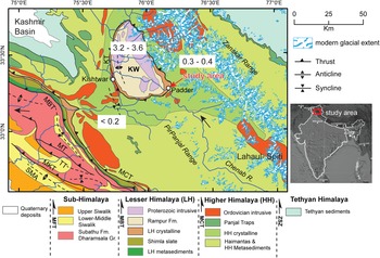
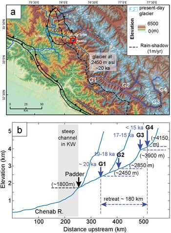
The study area chosen for this work, Padder town and surroundings, is situated along the southeastern margin of the Kishtwar tectonic window in the interior of Kashmir Himalaya. Located at an elevation of ~1770–1800 m above mean sea level (amsl), the area is drained by the Chenab River and its northern tributary, the Padder River (Fig. 2). From this point onwards, we shall use the term ‘Padder valley’ to refer to the study area. The Kishtwar Window exposes the Lesser Himalayan duplex, which is undergoing rapid exhumation at a rate of ~3.0–3.6 mm/yr for the last few million years (Gavillot et al., Reference Gavillot, Meigs, Sousa, Stockli, Yule and Malik2018). The eastern part of the window exposes quartzites of the Rampur Formation, intrusive granites, and highly sheared low- to medium-grade schists associated with the Main Central Thrust (MCT) shear zone (Fig. 2). In the hanging wall of the MCT, garnet- and staurolite-bearing Higher Himalayan crystalline rocks and farther upstream, the medium–high grade Higher Himalayan metasediments, known as the Haimantas, are exposed. The known exhumation rates from the Higher Himalaya are much lower than those of the Kishtwar Window (0.3–0.4 mm/y; Gavillot et al., Reference Gavillot, Meigs, Sousa, Stockli, Yule and Malik2018). The Chenab River, which originates in the Lahaul-Spiti region of the northern Himachal Pradesh, traverses ~350 km before reaching the Padder valley (Fig. 3a). The upstream reaches of the Chenab River and the southern flank of the Zanskar Range, which lie within the Higher Himalaya, are dominated by glaciers at present. During the last glacial maximum (LGM), the glacial extent was much greater, with most of the Higher Himalaya covered with ice (e.g., Kapannusch et al., Reference Kapannusch, Scherler, King and Wittmann2020). In contrast, the Lesser Himalayan domain is sparsely populated by glaciers at present. Previous studies suggest that the upper Chenab valley has been subjected to glacial advancement and retreat across centennial to millennial timescales (Kulkarni et al., Reference Kulkarni, Bahuguna, Rathore, Singh, Randhawa, Sood and Dhar2007; Eugster et al., Reference Eugster, Scherler, Thiede, Codilean and Strecker2016). Eugster et al. (Reference Eugster, Scherler, Thiede, Codilean and Strecker2016) constrained the advancement of the Chenab valley glacier using 10Be exposure ages from glacially polished Higher Himalayan bedrock (Fig. 3b). They reported glacial advancement down to ~2450 m above msl during the last glacial maximum (LGM), which remains as one of the lowest (w.r.t. elevation) known Himalayan glaciers during the LGM. The study area and surroundings receive 0.8–1.1 m/y rainfall (Bookhagen and Burbank, Reference Bookhagen and Burbank2006). There is no record of historical seismicity in the nearby regions in the upstream, nor any records of significant earthquakes (Mw>3.5) in the last few decades (International Seismological Centre, 2021; Supplementary Figure S1). However, based on the evidence of last few decades or few centuries, we cannot comment on the seismic situation that prevailed during the formation of the archive.
An overview geological map of the far-western Himalaya showing the regional lithology (modified after Steck, Reference Steck2003, and Gavillot et al., Reference Gavillot, Meigs, Sousa, Stockli, Yule and Malik2018) and glacial extent from the GLIMS (global ice measurements from space) global database (GLIMS Consortium, 2005 [updated 2018], https://doi.org/10.7265/N5V98602; see Raup et al., Reference Raup, Racoviteanu, Khalsa, Helm, Armstrong and Arnaud2007). Our study location is near the town of Padder, at the southeastern margin of the Kishtwar Window (KW). Note that the present-day glaciers are mostly nestled in the Higher Himalayan domain. Glacial coverage in the Higher Himalaya was more extensive during the LGM. Numbers in the white rectangles denote Quaternary exhumation rates (in mm/y) (adapted from Gavillot et al., Reference Gavillot, Meigs, Sousa, Stockli, Yule and Malik2018).

(a) Topographic map of the western Himalaya showing the glaciated landscape of the HH domain. The glacial extent (G1–G4) during and after LGM are plotted after Eugster et al., Reference Eugster, Scherler, Thiede, Codilean and Strecker2016. (b) Longitudinal profile of the Chenab River traversing the western Himalaya. Note that the Chenab valley records ~180 km retreat within a span of ca. 5 ka. Our study area lies at ~1800 m asl.

METHODS
Field findings: Sediment log, clast count, valley morphology
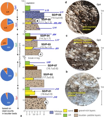
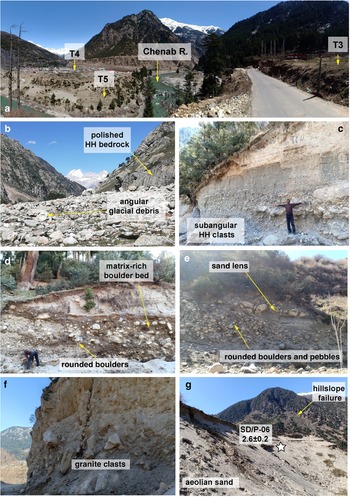
The Padder valley records a ~90–95 m thick aggraded sediment sequence (Fig. 4a). The valley is filled with sediments of varying grain size, ranging from boulders to silt. Based on lithology and stratigraphy (and chronology) we divided the entire sediment archive of the valley into five sub-packages, from Qp1–Qp5. Each of the sub-packages shows an overall fining-upward sequence. In the lower parts of the archive (Qp1 and Qp2), we observed angular to sub-angular boulders at the bottom, followed by gravels in the middle, and sandy silt at the top. In the middle (Qp3), we observed sub-rounded pebbles at the base and silt at the top. The matrix content in Qp3 is higher than Qp1–Qp2, with smaller grainsize. In the upper part of the archive, in Qp4, we observed sub-rounded to well-rounded pebbles at the base and sand at the top. The pebbles show imbrications and clearly bear a fluvial signature. The sand bodies are often isolated and coarse grained. In Qp5, the clasts at the base are leucogranites, and are highly angular and disoriented. Qp5 is topped by a thick layer of silt.
(a) Composite sediment log of the aggradation record in Upper Chenab Valley. We identified at least five fining-upward sediment packages (Qp1–Qp5) and identified those as different sediment pulses. Note the change in clast composition from Qp1 to Qp5 as the Lesser Himalayan component dominates the latter stages. (b–d) We also observed change in clast roundness, clast size, and matrix content of the coarsest layer of each package. Horizons labeled L and J represent samples used for statistical analysis of grain size (Fig. 7), grain shape (Fig. 7), and isotope fingerprinting (Fig. 9).

Clast counts were performed in the conglomeratic units of each package. For this, we used the grid method. We selected multiple 2m × 2m spots in the sediment archive and counted clasts that were >15 cm in diameter. The size filtering allowed us to count only the boulders and to cross-check our clast count by analysis of scaled photos taken in the field. Higher Himalayan (HH) and Lesser Himalayan (LH) clasts can be distinguished by their color—the Higher Himalayan clasts are darker and the granitic and quarzitic Lesser Himalayan clasts are whiter. We counted at least 250 clasts from each package and report the HH: LH clast ratio as pie charts (Fig. 4a).
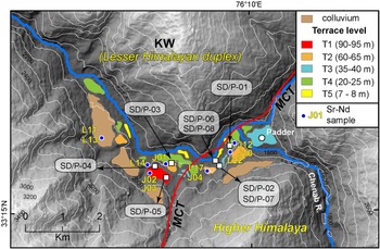
The valley-fill sediments are re-incised by the Chenab River, which has sculpted at least five terrace levels in the valley (Fig. 5). We classified the terraces (T1–T5) according to their decreasing heights from the river. At present, the river still incises the valley-fill sediments in the study area. Terrace T5, lying close to the river, has a ~3–4 m thick cover of very well-sorted, well-rounded fine-grained sand. The sand layer lacks lamination.
Topographic map of the study area showing different level of fluvial terraces, OSL and isotope sample locations near the confluence of the Chenab River and the tributary, the Padder River.

Field photographs. (a) Panoramic view of the lower terraces exposed near Padder. (b) Exposed glacial valley in the upper stretches of the Padder River. Angular glacial debris (HH crystalline rocks) are lying on the valley floor. (c) Glacial outwash sediments (Qp1) exposed in the study area showing a fining-upward sequence. (d) Photograph from Qp3 sediment sequence showing rounding of clasts and increase in matrix proportions. (e) Fluvial sequence from Qp4 showing clast-rich conglomeratic beds and isolated sand lenses. (f) Hillslope debris flow/landslide deposits of Qp5 only show the Lesser Himalayan granitic clasts. (g) T5 terrace exposing well-sorted aeolian sand.

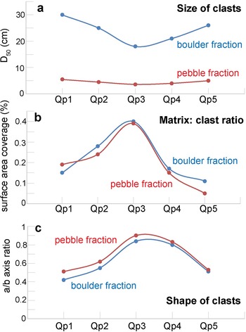
In addition to clast counts in the field, we also determined the median size of clasts in the boulder and pebble layers from each sedimentary package (Fig. 7a) and the shape of the clasts using the commonly used axis ratios (a/b axis ratio) (Fig. 7c). From field photographs, we estimated the matrix to clast ratio by comparing exposed surface area covered by clasts in the 2m × 2m grid used for clast count.
Graphs showing changes in (a) median grain size, (b) matrix:clast ratio, and (c) axis ratios representing clast roundness from sediment packages Qp1–Qp5.

Luminescence dating of terrace sediments
Optically stimulated luminescence (OSL) dating is a widely accepted method for assessment of sediment depositional ages across various depositional environments and has been successfully applied to Himalayan sediments despite its low sensitivity and tendency of heterogeneous bleaching (e.g., Fuchs and Owen, Reference Fuchs and Owen2008; Srivastava et al., Reference Srivastava, Kumar, Mishra, Meena, Tripathi, Sundriyal, Agnihotri and Gupta2013; Dey et al., Reference Dey, Thiede, Biswas, Chauhan, Chakravarti and Jain2021). To obtain the timing of deposition of sediments in Padder valley, we took seven samples from the medium-grained sand layers (SD/P01-P05 and SD/P07- P08) in terraces T1–T4 and one sample from the fine-grained sand layer in terrace T5 (SD/P06) for OSL measurement (Fig. 5).
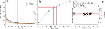
OSL samples were collected in GI pipes that were 9” long. Two inches from either end of the pipe were used for dose rate measurement and the rest of the samples were chemically treated for quartz extraction. Quartz grains of 90–150 μm size fraction from the samples were extracted using standard separation protocol (Aitken, Reference Aitken1998) in the Physical Research Laboratory, Ahmedabad. Twenty-four aliquots of each sample were measured using a Risø TL-OSL reader in the Physical Research Laboratory, Ahmedabad. The Equivalent dose (De) for each sample was measured using the OSL Double SAR (Single Aliquot Regenerative) protocol (Roberts, Reference Roberts2007). Test doses were set in the range of 25–120 Gy. The aliquots were considered for ED estimation only if: (1) recycling ratio was within 1 ± 0.1, (2) De error was <20%, (3) test dose error was <10%, and (4) recuperation was below 5% of the natural. Because all the samples show over dispersion values <20%, we used the Central Age Model (CAM) to estimate De (Bailey and Arnold, Reference Bailey and Arnold2006). Mean De ± 1σ for each of the samples is reported in Table 1 and Figure 8.
(a) Shine curve, (b) dose growth curve, and (c) radial plot for De estimation for sample SD/P-02. Note that the black circles represent the aliquots used for the mean ± standard deviation estimation of De; n represents the total number of aliquots that passed the filter criteria described in the methods section.

Details of OSL samples from Chenab valley and age calculation following a Central Age Model (after Bailey and Arnold, Reference Bailey and Arnold2006).

The dose rate was estimated using online software DRAC (Durcan et al., Reference Durcan, King and Duller2015) from the concentrations of Uranium (U), Thorium (Th), and Potassium (40K) (Table 1). Thick source ZnS (Ag) alpha counter was used for determining the elemental concentrations of Uranium and Thorium, while the Potassium concentrations were estimated using NaI (Tl) gamma ray spectrometry. Estimation of moisture content was done using the fractional difference of saturated versus unsaturated sample weight and rounded off to the nearest integer (Table 1).
Sr-Nd isotopic ratios
Eleven samples were collected from the silt-clay layers in the Qp1–Qp5 sediment packages. Samples were dissolved using the standard HF-HNO3-HCl dissolution protocol for silicates. Pure elemental Sr and Nd were separated from sample solutions by means of conventional cation exchange liquid chromatography with AG® 50W-X8 and Ln-spec resins from Biorad and Eichrom®, respectively, and using dilute HCl as elutants. Sr was further purified using Sr-spec resin from Eichrom® with water as elutant. Details of these experimental procedures are given in Chatterjee and Ray (Reference Chatterjee and Ray2017, Reference Chatterjee and Ray2018). 87Sr/86Sr and 143Nd/144Nd were measured on a Thermo Fisher make Triton Plus TIMS in a multi-collection (static) mode and were corrected for machine-induced mass fractionation using 86Sr/88Sr ratio of 0.1194 and 146Nd/144Nd ratio of 0.7219, respectively. The precision values of 87Sr/86Sr and 143Nd/144Nd analyses, based on measurements of international standards NBS-987 for Sr and JNdi-1 for Nd were ± 0.000005 (2σ) and ± 0.000003 (2σ), respectively (Sr-Nd isotope ratios are listed in Table 2 and data are given in Fig. 9a). Additional analytical information is provided in Singh et al. (Reference Singh, Ray, Jain and Mahala2022) and in the footnote of Table 2.
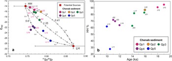
(a) Plot of εNd versus 87Sr/86Sr for sediment samples (labeled) from the Chenab River Valley terraces near Padder, Jammu & Kashmir. The data are compared with the average isotopic compositions (± 1σ) of rocks of the Higher Himalayan (HH) sequences and the Lesser Himalaya (LH) sequences of the region, which are the potential sediment sources for the Chenab River (data sources: Miller et al., Reference Miller, Klötzli, Frank, Thöni and Grasemann2000, Reference Miller, Thöni, Frank, Grasemann, Klötzli, Guntli and Draganits2001). The dashed lines are binary mixing curves between the two source endmembers, with fraction of the HH in the mixture marked. The italicized number on each curve is (SrA/SrB)/(NdA/NdB), where A and B stand for HH and LH, respectively. (b) Plot showing decreasing HH contribution with time.

Sr-Nd isotopic data for the Upper Chenab valley sediment samples.

Note: Sr and Nd isotope ratios were corrected for mass fractionation using 86Sr/88Sr = 0.1194 and 146Nd/144Nd = 0.7219, respectively. The long-term (n = 40) average values for NBS987 and JNdi-1 are 87Sr/86Sr = 0.710250 ± 0.000008 and 143Nd/144Nd = 0.512101 ± 0.000004 (±0.1 in εNd units), respectively, at the 2σ level of uncertainty. The rock standard BHVO-2 analyzed along with the samples yielded the following values: 87Sr/86Sr = 0.70348 and 143Nd/144Nd = 0.512968. εNd(0) = [(143Nd/144Nd)sample/(143Nd/144Nd)chondrite − 1]×104
RESULTS
OSL chronology of terrace sediments
OSL dates of the samples SD/P-01, SD/P-02, and SD/P-07, taken from the base of the valley-fill deposits (Qp1 and Qp2), yield depositional ages of 18.8 ± 0.9 ka, 17.2 ± 0.9 ka, and 16.1 ± 0.6 ka, respectively (Table 1). Samples SD/P-03 and SD/P-04, taken from the middle of the valley-fill sediments (Qp3), give depositional ages of 15.9 ± 1.6 ka and 14.3 ± 1.7 ka, respectively. Samples SD/P-05 and SD/P-08 taken near the top of the valley-fill sediments (Qp4) provide depositional ages of 11.3 ± 1.3 ka and 10.5 ± 0.8 ka, respectively. Sample SD/P-06 from the fine-grained sand layer exposed in terrace T5, near the riverbed, produced a depositional age of 2.6 ± 0.2 ka.
Clast counts in coarser fractions
Clast counts in the field from the conglomeratic layers show a decreasing HH contribution from the bottom to the top of the sediment log (Fig. 4a). The change in HH:LH ratio in Qp1 to Qp3 is gradual, whereas the HH contribution in Qp1 is ~95%, the HH contribution in Qp2 and Qp3 is ~88% and ~70%, respectively. However, in Qp4 and Qp5, the HH fractions are unexpectedly low—only ~21% in Qp4 and almost negligible (3%) in Qp5.
Clast shape and size analysis
Clasts in the bottom parts of the sequences Qp1 and Qp2 are larger (D50, the median grain-size in boulder beds, is 25–30 cm, and in pebble layers is 4.5–5.5 cm) than those in Qp3 (D50 in boulder beds is ~18 cm and in pebble layers is 3.6 cm) (Fig. 7). In the upper part of the archive, D50 values in boulder beds and pebble beds of Qp4 and Qp5 are 21–26 cm and 4–5 cm, respectively. The axis ratio of clasts is lower in both size fractions in Qp1 and Qp5 (0.4–0.5) compared to that in the middle of the section (0.8–0.9) (Fig. 7).
Isotopic fingerprinting of terrace sediments
The Sr isotopic ratio of the samples shows a narrow range of variation, 87Sr/86Sr = 0.757–0.810, whereas the Nd isotopic ratios show a larger variation (εNd = −27.2 to −14.7; Table 2). εNd values of the stratigraphically lower units are higher (−16.6 to −14.7) compared to those of the upper units (−27.2 to −21.8) (Fig. 9a).
DISCUSSION
We compiled our field, sedimentological, geochronological, and isotopic data for aggraded sediments in the Padder valley. We then compared our results with previously published records of glacial dynamics in the upper Chenab valley and global climate records to assess the role of deglaciation and monsoon intensity in the sediment aggradation observed in this part of the Himalaya.
Evolution of fluvial terraces in the Padder valley
The Padder valley records major aggradation during 20–10 ka (Table 1). The fining-upward sediment sequences (Qp1–Qp3) show sub-angular to sub-rounded clasts and poor imbrication and are identified as fluvially transported glacial outwash deposits (e.g., Maizels, Reference Maizels and Menzies2002). The deposits are constrained within a narrow valley and are laterally continuous, therefore, arguably not related to a braided channel. Therefore, each of the sediment packages can be considered as one major pulse of a sediment-transfer event. Isolated sand layers from Qp1– Qp3 show depositional ages varying between ca. 20–14 ka (Fig. 4a; Table 1). On the contrary, nicely rounded, polished, imbricated pebbles and cross-bedded sand bodies in Qp4 appear to be exclusively fluvial. In Qp4, the depositional ages range from ca. 11–10 ka. Qp5 is dominated by angular, disoriented granitic clasts of LH origin and is topped by a layer of fine silt. Qp5 is identified as a hillslope debris-flow deposit. Similar debris-flow deposits have been reported from the western margin of the KW (Dey et al., Reference Dey, Thiede, Biswas, Chauhan, Chakravarti and Jain2021). Qp5 is younger than 10 ka.
Clast counts in coarse fractions of the sediment archive hint at variable proportions of sediment sourcing from the HH and LH domains. The LH contribution is higher in the upper part of the archive. Isotopic source fingerprinting using 87Sr/86Sr and εNd in the silt fractions of the archive also suggests the same. A simple binary mixing model involving the Higher Himalayan sequences (HH) and the Lesser Himalayan sequences (LH) as two source endmembers (Fig. 9a) clearly suggests that the silt fractions in all sampled terrace sediments of the Chenab in the Padder valley were exclusively sourced from these two Himalayan domains. Model calculations also reveal that the (silt) sediment contribution from the HH to the valley decreased almost linearly with time since the LGM (ca. 20 ka; Fig. 9b).
Role of deglaciation in the sediment record
Glacial-interglacial cycles are linked to global solar insolation trends (e.g., Prell and Kutzbach, Reference Prell and Kutzbach1987; Huybers, Reference Huybers2006). Figure 1 shows low solar insolation during ca. 28–16 ka, which is known globally as the last glacial maximum (LGM). Eugster et al. (Reference Eugster, Scherler, Thiede, Codilean and Strecker2016) estimated the LGM glacial extent along the upper Chenab valley with surface-exposure dating of glacially polished bedrocks using 10Be. That study argued that at ca. 20 ka, the Chenab valley glacier had advanced down to ~2450 m amsl and was located only ~90 km upstream from the Padder valley (see point G1 in Fig. 3), and that during the next 5–6 kyr, the glacier had retreated ~180 km to reach ~4150 m amsl (see point G4 in Fig. 3b). Similar glacial retreats likely occurred in the northern tributaries originating from the arid Zanskar Range.
Sediment chronology in the Padder valley is synchronous with the published ages of glacial retreat post-LGM. Clast counts (Fig. 4a) and isotopic compositions (Fig. 9) confirm that the sediments (Qp1–Qp3) were primarily sourced from the HH domain from 20 ka until at least 14 ka. Decreasing clast-size, increasing grain roundness and matrix to clast ratio, and decreasing HH fraction from Qp1 to Qp3 hint at longer fluvial transport for the glacial outwash sediment with time. Decreasing fraction of the HH contribution probably was a result of increasing distance from the source to the sink. The field findings and analytical results nicely corroborate the published glacial retreat history of the Chenab valley glacier (Eugster et al., Reference Eugster, Scherler, Thiede, Codilean and Strecker2016). Moreover, the monsoon pressure index in the Indian Ocean and simulated total precipitation in the Himalaya during 20–14 ka were lower than that of the present day (Prell and Kutzbach, Reference Prell and Kutzbach1987; Dortch et al., Reference Dortch, Owen, Haneberg, Caffee, Dietsch and Kamp2009), which in turn suggests that the ISM had little control over the formation of Qp1–Qp3. Therefore, we relate the majority of sediment aggradation (~70 m) to deglaciation in the upper Chenab valley or southern flank of the Zanskar Range, located to the north of the Padder valley.
Effect of monsoon cycle on sediment aggradation and re-incision
The HH domain hosts the majority of the glaciers, therefore, it is expected to be affected by deglaciation more than the LH domain. It is generally thought that major deglaciation in the Himalaya had ceased by 14 ka and the extent of glaciation has remained almost unchanged since then (Eugster et al., Reference Eugster, Scherler, Thiede, Codilean and Strecker2016; Fig. 3a). As mentioned earlier, Qp4 (11–10 ka) has a prominent fluvial signature and has ~80% contribution from the LH in the pebble-boulder fraction (Fig. 4a) and 30–40% in the silt fraction (Fig. 9b). Therefore, Qp4 has more contribution from the LH domain, which didn't have glacial coverage post-LGM. Slight decrease in roundness and increase in clast size in comparison to Qp3, further suggest shorter transport for Qp4 sediment. Thus, Qp4 has a lower HH or glacial source, having sediments that originated from the non-glaciated hillslopes of the surrounding LH. The Early Holocene (12–8 ka) was characterized by strong monsoon, with monsoon pressure index up to 40% higher and the total simulated precipitation 10% higher than the present day (Prell and Kutzbach, Reference Prell and Kutzbach1987; Dortch et al., Reference Dortch, Owen, Haneberg, Caffee, Dietsch and Kamp2009; Gebregiorgis et al., Reference Gebregiorgis, Hathorne, Sijinkumar, Nath, Nürnberg and Frank2016). Many of the western Himalayan valleys exhibit aggradation during this period (e.g., Bookhagen et al., Reference Bookhagen, Fleitmann, Nishiizumi, Strecker and Thiede2006; Srivastava et al., Reference Srivastava, Tripathi, Islam and Jaiswal2008; Dey et al., Reference Dey, Thiede, Schildgen, Wittmann, Bookhagen, Scherler, Jain and Strecker2016). Therefore, aggradation of Qp4 can be attributed to the Early Holocene (12–10 ka) intensified ISM.
An almost linear decrease in the HH contribution in the sediment signal with time (Fig. 9b) points to two possible scenarios. (1) Increasing distance from the sediment source—The Higher Himalayan glaciers were the major source of sediments during the entire aggradation phase (Qp1–Qp4). However, as the glaciers retreated upstream, the source to sink distance became >300 km by the Early Holocene. Higher HH contribution in the silt fraction versus in the clast fraction supports the claim of longer fluvial transport of the HH-derived sediment. (2) Shift in erosional domain—The steeper hillslopes of the HH domain would have aided enhanced erosion due to a stronger monsoon. However, in a recently published study from the Dhauladhar region in western Himalaya, Dey et al. (Reference Dey, Thiede, Biswas, Chauhan, Chakravarti and Jain2021) have shown that the moderately steep regions are more sensitive to climate change and, therefore, the response to change in monsoon intensity was higher in the LH domain. That is why in Qp4, the abundance of HH clasts is lower (60–70%) than that in Qp1–Qp3 (>80%) (Fig. 7b).
Since 8–10 ka, the Padder valley experienced recurring re-incision of transiently stored sediment. Each re-incision phase was marked by formation of fluvial-fill terraces (T1–T4). Holocene staircase terraces are common in the Himalayan valleys across wet to semi-arid landscapes (e.g., Pratt-Sitaula et al., Reference Pratt-Sitaula, Burbank, Heimsath and Ojha2004; Bookhagen et al., Reference Bookhagen, Fleitmann, Nishiizumi, Strecker and Thiede2006; Sinha et al., Reference Sinha, Suresh, Kumar, Dutta and Arora2010; Dutta et al., Reference Dutta, Suresh and Kumar2012, Reference Dutta, Mujtaba, Saini, Chunchekar and Kumar2018; Dey et al., Reference Dey, Thiede, Schildgen, Wittmann, Bookhagen, Scherler, Jain and Strecker2016; Chahal et al., Reference Chahal, Kumar, Sharma, Singhal, Sundriyal and Srivastava2019). Barring a few instances (e.g., Sinha et al., Reference Sinha, Suresh, Kumar, Dutta and Arora2010; Dutta et al., Reference Dutta, Suresh and Kumar2012), episodic weakening of the ISM has been linked to the formation of these Holocene terraces. Thus, the Padder valley morphology appears to attest to a synchronized Holocene sediment removal from the Himalayan valleys.
Debris flows and landslides during the Early Holocene
Landslides triggered by earthquakes are as common as rainfall-driven landslides in the High mountains (e.g., Bookhagen et al., Reference Bookhagen, Thiede and Strecker2005a, Reference Bookhagen, Thiede and Streckerb; Parkash, Reference Parkash, Margottini, Canuti and Sassa2013). Landslides and hillslope debris flows that define the Qp5 aggradation sequence occurred in the Early Holocene. Clast counts and valley morphology confirm that the source of sediments in Qp5 is the valley walls of the surrounding LH domain. Negligible HH contribution in the clast fraction and much-reduced HH component in the silt fraction (Fig. 9) could possibly indicate reworking and incorporation of Qp4 sediments into the mass flow. The Early Holocene period is characterized by a strong ISM. Increased monsoon strength could have activated the meta-stable hillslopes of the eastern edge of the KW. Seismic epicenter maps of this region (Supplementary Fig. S3) show considerable numbers of small- to moderate-magnitude earthquakes (Mw: 3–5) in this region, suggesting possible occurrences of similar activity in the past as well. Penecontemporaneous deformation structures in soft sediments are common features in the Himalayan sediment archives affected by concurrent seismicity (e.g., Kotlia and Rawat, Reference Kotlia and Rawat2004; Phartiyal and Sharma, Reference Phartiyal and Sharma2009; Mugnier et al., Reference Mugnier, Huyghe, Gajurel, Upreti and Jouanne2011). Absence of penecontemporaneous deformation structures in the studied sediment sequences doesn't confirm the role of seismicity; however, we are not able to completely rule out its possibility. Similar conclusions were drawn by Dortch et al. (Reference Dortch, Owen, Haneberg, Caffee, Dietsch and Kamp2009) where they studied large landslides in the Himalaya. To add to this, decadal- to centennial-scale seismic data cannot be extrapolated up to 20 ky ago when the deposition initiated. Therefore, the role of tectonics cannot be verified with the available data.
Large-scale seismic activity in the Himalaya could be responsible for the formation of landslide-dammed lakes (e.g., Korup et al., Reference Korup, Montgomery and Hewitt2010; Kumar et al., Reference Kumar, Jamir, Gupta and Bhasin2021). However, there are no lacustrine deposits stored at the base of the aggradation sequence in the Padder valley. Lacustrine deposits could well have been completely incised by the river or buried by the aeolian sediments near the present-day stream. Not finding a lacustrine deposit certainly doesn't mean that it was not there. However, because we could not find any evidence, the role of landslide-damming cannot be evaluated with the available dataset and field findings. We have observed several modern-day landslides/hillslope failures in the eastern fringes of the KW; however, they are much smaller in size and probably are incapable of blocking the Chenab River.
Role of aridity during the Late Holocene
The lowest terrace (T5) records a ~4 m thick fine-grained sand capping (Fig. 5f). The sand capping is devoid of any recognizable laminations, the grain-size is small (80 ± 20 μm) and sorting is high. A single depositional age from this aeolian sand layer suggests a Late Holocene age (age-SD/P-06: 2.6 ± 0.1 ka). The De estimates of sample SD/P-06 form a cluster resulting a low over-dispersion value (OD ~6%; Table 1), which suggests that the sample was uniformly (well) bleached. We interpret the sand layer as a loess deposit. Surface-draping aeolian deposits are common in the arid western Himalaya (e.g., Kumar et al., Reference Kumar, Srivastava and Meena2017). Based on OSL-dated moraines, Bisht et al. (Reference Bisht, Ali, Rana, Singh, Sundriyal, Bagri and Juyal2017) proposed a protracted arid phase during ca. 5–3 ka in the western Himalaya. A previous study by Khan et al. (Reference Khan, Meena, Sundriyal and Sharma2022) suggested the existence of a period of aridity in the Himalaya during 4–1 ka. Although we have very limited age control, the loess deposit in the Padder valley could be broadly linked with this dry phase.
CONCLUSIONS
Combining the results from our field observations and analytical results, in conjunction with inferences made by earlier studies, we reach the following conclusions. (1) Sediment aggradation in the Padder valley happened during 20–10 ka and was followed by recurring incision, leading to formation of staircase fill terraces. (2) Field evidence and analytical results neither can verify nor can rule out any tectonic trigger behind the aggradation. Rather, the observed sediment aggradation and re-incision followed the trend of global climatic fluctuations, suggesting climatic control on sediment transfer. (3) Initial stages of terrace sedimentation were dominated by fluvially transported glacial outwash sediments that bore signatures of the Higher Himalayan provenance. In contrast, the upper part of the archive exhibited reduced influence of the glaciated Higher Himalaya and contained a significant contribution from the non-glaciated Lesser Himalayan sources. Overall, glacial sediments dominate (~70%) the total sediment deposition in the valley. (4) The decrease in the Higher Himalayan contribution to the sediment archive with time could be attributed either to retreat of the Chenab valley glacier or to increased erosion of the Lesser Himalayan domain during the Early Holocene, or a combination of both. The first is supported by the 180 km glacial retreat during 20–15 ka in the Upper Chenab valley, and the second is backed by increased erosion in the Lesser Himalayan domain.
This study highlights a dominant role of glacial dynamics on the aggradation pattern observed in a fluvial valley in the Higher Himalaya. The role of glaciers needs to be investigated further in other fluvial networks to understand the complexity of sediment transfer in response to climate change.
Acknowledgments
S. Dey is supported by DST-INSPIRE faculty research grant by the Department of Science and Technology, India (grant #DST/INSPIRE/04/2017/003278). The authors acknowledge help from T. Tsering, C. Singh, S. Das, and A. Das during fieldwork. The authors thank J. Dortch and an anonymous reviewer for insightful comments and suggestions on a previous version of the manuscript.
Supplementary Material
The supplementary material for this article can be found at https://doi.org/10.1017/qua.2022.57