Implications
Random regression models (RRMs) applying spline functions could be an option to model weights until mature age, as these functions are less susceptible to the problems frequently observed with orthogonal Legendre polynomials. However, to date there are no studies that have applied RRM on B-spline functions to estimate genetic parameters for weights in Nellore cattle. The results of this research showed that RRMs using B-spline functions revealed similar description of the trajectory of the variances and heritability estimates. Moreover, random regression on B-spline functions required lower computational requirement and faster convergence in relation to Legendre polynomials or multi-trait analysis. In genetic evaluation programs, with large data set, the application of RRMs using B-spline functions could still be advantageous compared with Legendre polynomials.
Introduction
Random regression models (RRMs) based on Legendre polynomials have been used to study genetic parameters for growth traits in beef cattle (Albuquerque and Meyer, Reference Albuquerque and Meyer2001; Nobre et al., Reference Nobre, Misztal, Tsuruta, Bertrand, Silva and Lopes2003; Arango et al., Reference Arango, Cundiff and Van Vleck2004; Meyer, Reference Meyer2004, Nephawe, Reference Nephawe2004; Boligon et al., Reference Boligon, Mercadante, Forni, Lobo and Albuquerque2010). These models present the advantage of using all records of the animal and of eliminating the need for the correction of weights for standard ages. In addition, it provides more accurate estimates of breeding values for any age within the interval of the records considered when compared with conventional multi-trait models (Tier and Meyer, Reference Tier and Meyer2004).
Over the past few years, various researchers have pointed out that the use of random regression analysis based on Legendre polynomials to model weights in beef cattle may present some undesired properties, such as the need for employing high-degree polynomials and large increases of (co)variances along the curve (Meyer, Reference Meyer1999; Nobre et al., Reference Nobre, Misztal, Tsuruta, Bertrand, Silva and Lopes2003; Sakaguti et al., Reference Sakaguti, Silva, Quaas, Martins, Lopes and Silva2003), especially at ages with a small number of weight records.
According to Meyer (Reference Meyer2005a), analysis of weight records in beef cattle using RRMs with cubic, quadratic or even higher order polynomials has resulted in erratic and implausible estimates of variance components and genetic parameters. These problems are mainly observed in the case of data sets that contain a small number of records for the last ages, as adult weights, associated with a small number of records per animal, and in the case of analyses in which the number of records available for the animals is smaller than the order of the fitted polynomials. In this sense, Boligon et al. (Reference Boligon, Mercadante, Forni, Lobo and Albuquerque2010), using Legendre polynomials to model changes in variances with age for weights from birth to adulthood, reported convergence problems with the increase in polynomial order.
In this respect, RRMs applying spline function offer a viable method to model weight records until mature age, as these functions are less susceptible to the problems frequently observed with orthogonal Legendre polynomials. According to Meyer (Reference Meyer2000), spline function permitted the fitting of lower-degree polynomials in short segments of the growth trajectory, thus resulting in greater flexibility when fitting seasonal fluctuations in cattle growth.
One particular type of spline function is called B-splines, which are preferred because of their excellent numerical properties (Ruppert et al., Reference Ruppert, Wand and Carroll2003). According to Rice and Wu (Reference Rice and Wu2001), B-splines are adequate to model random effects in mixed model analyses and are also efficient in estimating covariance functions.
In beef cattle, spline functions have been used to describe genetic variations in the growth of Angus cattle using weights from birth to 820 days of age (Meyer, Reference Meyer2005b), in Gelbvieh from birth to 1 year of age (Iwaisaki et al., Reference Iwaisaki, Tsuruta, Misztal and Bertrand2005) and in Polled Hereford dams from 1.5 to 7 years of age (Meyer, Reference Meyer2005c). Similarly, Sánchez et al. (Reference Sánchez, Misztal, Aguilar and Bertrand2008) applied linear spline RRMs to analyze weights of crossbred animals from birth to 1 year of age and showed that these models can also be used for genetic evaluation of multi-breed populations.
In Brazil, Baldi et al. (Reference Baldi, Alencar and Albuquerque2010) compared estimates of (co)variance functions for weights of Canchim females from birth to adulthood obtained by random regression using Legendre polynomials or B-splines. The results showed that B-spline functions provided a better description of the trajectory of variance estimates than Legendre polynomials, especially at older ages. However, there are no reported studies in the literature applying RRMs on B-spline functions to estimate genetic parameters for weight records in Nellore cattle.
Most Brazilian beef cattle are raised on range conditions, characterized by high temperatures and low-quality pastures. Of late, there have been concerns about consequences of selection to increase weights at young ages on cow size, which could result in higher costs to maintain the cow herd. In addition, for low-input environment, medium-sized cows seem to be advocated (Jenkins and Ferrell, Reference Jenkins and Ferrell1994). In this scenario, to maintain desirable adult size it is necessary to consider adult weight in beef cattle selection indices. However, there are difficulties to include adult weights in genetic evaluations because of the scarcity of weight records at later ages and the lack of adequate models to estimate (co)variance components at mature ages. Apparently, RRMs on B-spline functions offer advantages over the Legendre polynomials and the traditional finite dimensional models (Tier and Meyer, Reference Tier and Meyer2004) and could be used for genetic evaluation of growth traits.
The objective of this study was to estimate covariance functions for direct and maternal additive genetic effects, animal and maternal permanent environmental effects, and subsequently, to obtain genetic parameters for growth traits in Nellore cattle, from birth to adulthood, using RRMs on B-splines of animal age.
Material and methods
Data
The data used in this study were obtained from eight herds located in the State of São Paulo that are part of the Nellore Breeding Program (PMGRN/Nellore Brasil), where a genetic evaluation program started in 1987. The animals were weighed at intervals of 45 days from birth to yearling, and those remaining in the herds as seed stock continue to be weighed routinely at this interval. In the case of the data set used here, births occurred throughout the year, with a larger number of births during Spring (September to November) and Summer (December to February). The animals were weaned on average at 240 days of age. Only weight records of animals reared on pasture without supplementation and nursed by their biological mothers were included in the analysis. Age of dam at calving ranged from 2 to 24 years and 13 age classes were considered for analysis, because the last class included dams aged 15 years or older at calving.
The contemporary group for records from birth to 3 years of age was defined including animals born on the same farm, year and season of birth, and belonging to the same group for age at recording (birth and every 45 days of age). Consequently, the variation in age within the contemporary group was less than 45 days. After 3 years of age, the contemporary group consisted of farm, year and season of birth and year and season of recording. Weight records outside the intervals given by the mean of the contemporary group ± 3 s.d. were excluded. Contemporary groups containing fewer than eight animals were excluded, for a total of 2693 contemporary groups.
Animals with fewer than five weight records were excluded. The mean number of records per animal was 10.07, with a maximum of 43. There were 813, 2133, 1243, 1138, 528, 282 and 2008 animals with 5, 6, 7, 8, 9, 10 and 11 to 43 weight records, respectively, corresponding to 63.83%, 48.57% and 34.60% of animals with at least 7, 8 and 9 records, respectively.
The data set analyzed consisted of 81 712 weight records from birth to 8 years of age, comprising 8144 females, daughters to 470 sires and 5185 cows. The relationship matrix was constructed using information from all generations available and contained 12 596 animals.
Analysis
All models included direct and maternal genetic and animal and maternal permanent environmental effects as random effects, in addition to residual effects. The random effects were modeled using B-spline functions (Marx and Eiler, Reference Marx and Eilers1998). Contemporary group and linear and quadratic effects of dam age at calving within the age class of the animal (five classes: 2 to 3, 4 to 5, 6 to 8, 9 to 11, 12 to 24 years of age) were included as fixed effects.
A fourth-order orthogonal Legendre polynomial was used to model the population's mean growth trajectory. Residual variances were modeled considering five age classes (1, 2 to 240, 241 to 550, 551 to 730 and 731 to 2889 days). The matrix representation of the models is

where y is the vector of observations, b is the vector of fixed effects, a is the vector of random coefficients for additive direct effects, m is the vector of random coefficients for additive maternal effects, pe is the vector of random coefficients for animal permanent environmental effects, mpe is the vector of random coefficients for maternal permanent environmental effects, e is the vector of residual effects and X, Z1, Z2, W1 and W2 are the corresponding incidence matrices. The model is based on the following assumptions:
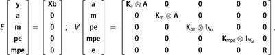
where Ka, Km, Kpe and Kmpe are (co)variance matrices between random regression coefficients for additive direct, additive maternal and animal and maternal permanent environmental effects, respectively, A is the relationship matrix, I is an identity matrix, N A is the number of animals for which records are available, N M is the number of dams with progeny records, ⊗ is the Kronecker product between matrices and R is a block diagonal matrix containing residual variances. Correlations between random regression coefficients for different effects were set to zero.
The B-spline function can be defined recursively (Meyer, Reference Meyer2005b), with basis functions of degree p = 0 assuming values of unity for all points in a given interval; otherwise, the value is zero. For the kth interval given by knots Tk and Tk < Tk + 1,

High-degree basis functions, Bk,p for p > 0, are then determined from the values of the lower degree basis functions, already evaluated, and the width of the adjoining intervals between knots (Meyer, Reference Meyer2005b). According to De Boor (Reference De Boor2001), the function can be described as

Linear (L), quadratic (Q) and cubic (C) polynomials were considered for each individual segment, with basis functions of degree p = 1, 2 and 3, respectively. Polynomials of the same degree were included in the model for all random effects. The m knots were chosen to divide the age at recording into m−1 equally spaced intervals and the external knots are located in classes 1 and 2889 for all models. Up to seven knots (six segments) were used for direct additive genetic and permanent environmental effects of the animal, with the same number of knots fitted for both effects. A single segment with two knots at the end points of the curve was used for maternal genetic and permanent environmental effects.
The number of random regression coefficients to model the trajectory of the linear, quadratic and cubic basis functions is given by m, m + 1 and m + 2, respectively. The nomenclature of the RRMs follows the pattern ‘BSX k a, k m, k pe, k mpe’, where X = L, Q or C, that is, the degree of the polynomial segment, and k a, k m, k pe and k mpe are the specific numbers of random regression coefficients for direct additive genetic, maternal genetic and animal and maternal permanent environmental effects, respectively. Thus, model BSL3232 consists of a linear B-spline function with three random regression coefficients for direct additive genetic and permanent environmental effects of the animal, and two random regression coefficients for maternal genetic and permanent environmental effects.
The covariance components and genetic parameters of the models were estimated by the restricted maximum likelihood method using the Wombat statistical program (Meyer, Reference Meyer2006). Direct additive genetic variances for weights at different ages  were obtained using

where fi′ is the vector of covariates corresponding to the B-spline function of age at recording in days, and Λ A is the matrix of direct additive genetic covariances between random regression coefficients. Maternal genetic, animal and maternal permanent environmental variances were obtained in a similar manner replacing Λ A by Λ M, Λ PE or Λ MPE, respectively. The Λ M, Λ PE and Λ MPE are the matrices of maternal genetic, animal and maternal permanent environmental covariances between random regression coefficients, respectively. The residual variances  were considered to change with age (described by five age classes). Thus, direct heritabilities of weights at different ages
 were calculated using the equation:

The same equation shown above was used to estimate maternal heritability  and animal
 and maternal
 permanent environmental variances as a proportion of total phenotypic variances, replacing the numerator of this equation by
 ,
 or
 , respectively (for details see Meyer, Reference Meyer2001; Mrode, Reference Mrode2005).
The models were compared using the Akaike information criterion (AIC) and the Schwarz–Bayesian information criterion (BIC; Schwarz, Reference Schwarz1978), and by the analysis of variances and correlations estimated for weights at the different ages considered. The AIC and BIC considered the lack of fit and the number of parameters estimated in the model. The AIC can be used to compare models including the same fixed effects but different variance structures. The judgment is the same in the case of the BIC, but this criterion attributes a higher penalty to models containing a larger number of parameters than the AIC. The information criteria are calculated as follows:
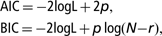
where p is the number of parameters in the model, N is the total number of observations, r is the rank of the incidence matrix of fixed effects in the model and logL is the logarithm of the likelihood function. Lower values for AIC and BIC indicate a better fit.
The results obtained with the B-spline functions were compared with those obtained using random regression on fourth- and sixth-order orthogonal Legendre polynomials for direct additive genetic and permanent environmental effects of the animal, respectively, and on third-order polynomials for maternal genetic and permanent environmental effects (Leg4363) as proposed by Boligon et al. (Reference Boligon, Mercadante, Forni, Lobo and Albuquerque2010). The same fixed effects were considered for all RRM.
A multi-trait analysis was also performed using a finite dimension model for weights at birth, weaning, yearling, 18 months of age and 2, 3, 4, 5 and 6 years of age. The model for all traits included direct additive and maternal genetic effects, maternal permanent environmental effects and residual effects as random effects. Contemporary group (farm, year and season of birth) and linear and quadratic effects of animal age at recording (except for weight at birth) and dam age at calving were included as fixed effects. The covariance between direct and maternal genetic effects was set to zero in line with the suggestion of Albuquerque and Meyer (Reference Albuquerque and Meyer2001) and Meyer (Reference Meyer2005b). Moreover, in Brazil this covariance is assumed to be zero in most of beef cattle evaluation programs. For more details, the multi-trait analysis applied was reported by Boligon et al. (Reference Boligon, Albuquerque, Mercadante and Lobo2009), using the same data set.
Results and discussion
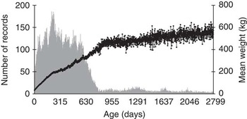
Weights increased with age, with a decrease in the growth rate after weaning, and a practically linear growth rate after 800 days of age (Figure 1). A marked decline in the number of animals was observed after 600 days of age, a finding suggesting that many farms only weigh females until they enter the first breeding season.
Number of records (bars) and mean weight (line) according to age.

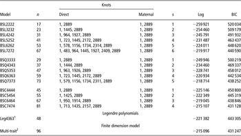
The two different information criteria to compare the models (AIC and BIC) indicated the same models, and thus only the BIC results were shown. Table 1 summarizes the results of the model comparisons using the logarithm of the likelihood function (logL), and BIC obtained for the models used. The number of parameters ranged from 17 to 81 in the models studied. The logarithm of the likelihood function (logL) improved as the number of parameters in the models increased, irrespective of the degree of the function. Similar results were reported by Meyer (Reference Meyer2005b) and Baldi et al. (Reference Baldi, Alencar and Albuquerque2010) using B-splines (linear, quadratic and cubic) to model the growth trajectory of Angus cattle from birth to 821 days of age and with Canchim females from birth to 8 years of age, respectively.
Models, number of parameters (n) in the model, position of knots, number of segments (s), likelihood function (log), and Schwarz–Bayesian information criterion (BIC) obtained for random regression models using B-splines and Legendre polynomials

1Legendre polynomials: 4, 3, 6 and 3 correspond to the order of the regression coefficients for direct additive and maternal genetic effects and animal and maternal permanent environmental effects, respectively.
2Weights at birth, weaning, yearling, 18 months of age and 2, 3, 4, 5 and 6 years of age.
None of the RRMs on B-splines as base functions with similar or lower number of parameters than the Leg4363 model had fitted better (Table 1). Therefore, applying RRMs on B-spline functions, a higher number of parameters were needed to reach a similar fit as Leg4363 model (Table 1). These results were in agreement with those reported by Meyer (Reference Meyer2005a), that even with relatively few knots RRMs on B-spline functions tend to involve a larger number of coefficients than models fitting Legendre polynomials.
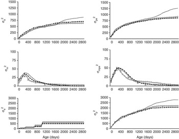
The logarithm of the likelihood function and the BIC results indicated that BSC7474 model, with 81 parameters, fitted the data best. However, this model presented implausible phenotypic variance estimates at extreme ages, compared with multi-trait and Leg4363 models (Figure 2). Alternatively, the model BSQ5353, with 47 parameters, showed variance component estimates similar to those from Leg4363 and multi-trait analysis. Increasing the number of knots or the polynomial order improved BIC; however, the variance estimates showed an unexpected behavior for later weights (not shown). Meyer (Reference Meyer2005b) also reported high and implausible residual and phenotypic variances at more advanced ages when weights were fitted using a cubic B-spline function. It should be emphasized that in the case of B-spline functions a good fit of the data depends, in addition to the order of the individual segments, on the data structure, with problems mainly being observed when the data are distributed irregularly.
Estimates of direct additive genetic  , maternal genetic
 , animal permanent environment
 , maternal permanent environment
 , residual
 and phenotypic
 variance components obtained with models BSC7474 (—), BSQ5353 (▪), Leg4363 (○) and by multi-trait analysis (
 ).

The direct additive genetic variances obtained by BSC7474, BSQ5353, Leg4363 and multi-trait models were similar until almost 5 years of age (Figure 2). However, after this point, the additive direct variance estimates obtained with the BSC7474 model were higher than those estimated with BSQ5353 with Leg4363 models. Similar results were reported by Baldi et al. (Reference Baldi, Alencar and Albuquerque2010) with weight records from birth to mature age in cows of Canchim breed. These authors reported that for weights measured after 6 years of age, RRMs on B-spline functions fitting cubic regression showed lower additive direct variance estimates than those obtained with B-spline functions fitting quadratic regression or Legendre polynomials.
Using weight records of Gelbvieh cattle from birth to 365 days of age, Iwaisaki et al. (Reference Iwaisaki, Tsuruta, Misztal and Bertrand2005) reported similar direct additive genetic variance estimates obtained by random regression on linear spline functions or by multi-trait analysis (weights at birth, weaning and 1 year of age). For ages with enough number of weight records, no important differences in variance component estimates are expected when random regression on B-spline or Legendre polynomials as base functions were applied (Meyer, Reference Meyer2005b).
Similar animal permanent environmental variance estimates were obtained for all RRMs until almost 5 years of age. After this age, the BSQ5353 showed lower animal permanent environmental variance estimates than those obtained with BSC7474 (Figure 2). Similar to the studies of Meyer (Reference Meyer2005b) and Baldi et al. (Reference Baldi, Alencar and Albuquerque2010), the use of quadratic B-spline functions permitted a better control of the variances of animal permanent environmental effects compared with fits obtained with cubic B-spline functions and Legendre polynomials.
The maternal genetic and permanent environmental variance estimates with BSC7474, BSQ5353 and using Legendre polynomials (Leg4363) or multi-trait analysis showed similar trend (Figure 2). For these models, higher variances were estimated for weights close to 240 days of age, followed by a decline after this age and variances of zero at older ages. Similar to this study, Albuquerque and Meyer (Reference Albuquerque and Meyer2001) observed that maternal genetic variance estimates increased until 150 days of age in Nellore cattle and remained practically constant until 240 days of age, followed by a decrease thereafter.
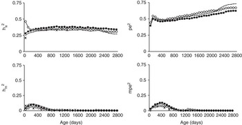
Except for the beginning of the study period (first 60 days), the heritability estimates for direct additive genetic effects obtained using the models BSC7474, BSQ5353 and Leg4363 and by multi-trait analysis showed the same trend (Figure 3). For all ages, direct heritability estimates obtained by BSC7474 model were slightly lower than those obtained with other models. Direct heritability estimates obtained by multi-trait analysis ranged from 0.23 (for weight at birth) to 0.35 (for weight at 5 and 6 years of age). In contrast, heritabilities obtained with model BSQ5353 presented an increase from birth (0.28) to yearling (0.38) and remained practically constant until 8 years of age (0.35). Using random regression on B-spline functions, Meyer (Reference Meyer2005b) reported higher direct heritabilities when compared with those obtained by single-trait analysis, especially for weights from weaning to 365 days of age. On the other hand, Iwaisaki et al. (Reference Iwaisaki, Tsuruta, Misztal and Bertrand2005) found higher direct heritability estimates by multi-trait analysis for weights at birth, weaning and 1 year of age (0.52, 0.36 and 0.59, respectively) compared with those obtained using linear spline functions (0.51, 0.28 and 0.48, respectively).
Estimates of direct (h a2) and maternal heritability (h m2) and estimates of animal (pe2) and maternal (mpe2) permanent environmental variance as a proportion of total phenotypic variance obtained with models BSC7474 (—), BSQ5353 (▪) and Leg4363 (○) and by multi-trait analysis ( ).

In Brazil, using random regression on B-spline functions for weights of Canchim females from birth to 8 years of age, Baldi et al. (Reference Baldi, Alencar and Albuquerque2010) observed an increase in the direct heritability estimates from birth to 450 days of age, followed by a small decline, remaining practically constant after 3 years of age.
Except at the end of the period studied, the estimates of animal permanent environmental variances as a proportion of total phenotypic variance were similar applying random regression on B-splines (BSC7474 and BSQ5353) or models fitting Legendre polynomials (Figure 3). For weights obtained after 5 years of age, the BSC7474 model showed a slight increase in animal permanent environmental variance as a proportion of phenotypic variance. Using the BSQ5353 model, the animal permanent environmental variances as a proportion of phenotypic variance increased from birth (0.39) to 120 days of age (0.50), presented a small decrease at about 300 days of age and then tended to increase slightly until the end of the study period. Similarly, Baldi et al. (Reference Baldi, Alencar and Albuquerque2010) reported an increase in animal permanent environmental variance as a proportion of phenotypic variance at the end of the study period. However, in contrast to this study, wider oscillations at the beginning of the study period were reported by these authors. According to Meyer (Reference Meyer2005b), B-spline functions are less susceptible to end-of-range problems, especially for animal permanent environmental effects, than orthogonal polynomials when modeling the growth curve of beef cattle.
For weight at birth, the maternal genetic heritabilities estimated by RRMs using B-spline functions or Legendre polynomials were lower than those obtained by multi-trait analysis (Figure 3). After birth, the maternal heritability estimates obtained by random regression on B-splines (BSC7474 and BSQ5353) increased until close to weaning (240 days of age) and decreased thereafter. Values of practically zero were observed after 365 days of age. In contrast to the present findings, Meyer (Reference Meyer2005b) and Iwaisaki et al. (Reference Iwaisaki, Tsuruta, Misztal and Bertrand2005) observed lower maternal genetic heritabilities when using spline functions compared with those obtained using a finite dimension model (single- or multi-trait analysis).
Maternal permanent environmental variances as a proportion of phenotypic variance estimated with the RRMs using B-spline functions followed the same trend as those obtained by multi-trait analysis (Figure 3). In contrast, the estimates obtained by random regression on Legendre polynomials were generally lower and close to zero. Meyer (Reference Meyer2005b) using RRMs on B-splines reported lower maternal permanent environmental variance estimates as proportions of phenotypic variances than those obtained with finite dimensional models.
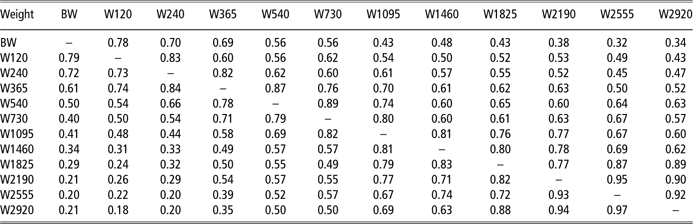
The direct and maternal genetic correlation estimates between weights from birth to adulthood obtained for both B-spline models were very similar. Thus, the genetic and maternal correlation obtained with model BSQ5353 are shown in Table 2. The genetic correlation estimates decreased with increasing distance between weights. The direct genetic correlations obtained were higher than 0.5 for most ages. These results suggest that selection for weights at any age should alter the adult weight of females in the same direction. Thus, adult weight would be subject to marked increases as a response to selection for higher weights at younger ages, such as weaning and yearling, traits that have received greater emphasis in selection indices used for beef cattle in Brazil.
Estimates of direct additive genetic (above the diagonal) and maternal (below the diagonal) correlations between weights from birth to adulthood obtained for model BSQ5353

BW: weight at birth.
W120, W240, W365, W540, W730, W1095, W1460, W1825, W2190, W2555 and W2920: weight at 120, 240, 365, 540, 730, 1095, 1460, 1825, 2190, 2555 and 2920 days of age, respectively.
Using Gelbvieh weight records from birth to 365 days of age, Iwaisaki et al. (Reference Iwaisaki, Tsuruta, Misztal and Bertrand2005) reported similar direct genetic correlations estimated by multi-trait analysis and random regression on spline functions. However, the estimated correlations between all weights were lower than those obtained in this study. In Brazil, Baldi et al. (Reference Baldi, Alencar and Albuquerque2010), using B-spline functions, also reported higher direct genetic correlations between adjacent weights and the estimated correlations between weights of females from birth to 8 years of age were generally similar to those observed in this study.
Using B-spline functions for weights from birth to 820 days of age, Meyer (Reference Meyer2005b) observed small oscillations in direct genetic and direct permanent environmental correlations at ages in which knots were inserted. Iwaisaki et al. (Reference Iwaisaki, Tsuruta, Misztal and Bertrand2005) stated that RRMs on linear spline functions allow to estimate genetic parameter with smoother trajectories as spline functions fitted the data better at ages with lower number of records.
The estimates of maternal genetic correlations between weights from birth to 365 days of age were high, ranging from 0.61 to 0.84. Similarly, correlation estimates between weights after 365 days of age until 8 years of age also presented a moderate-to-high magnitude (Table 2). These results suggest that maternal effects at early ages are controlled by the same genes. Also using B-spline functions, Baldi et al. (Reference Baldi, Alencar and Albuquerque2010) reported higher maternal genetic correlations, especially between weights obtained after weaning (0.99). On the other hand, Albuquerque and Meyer (Reference Albuquerque and Meyer2001), using RRM fitting Legendre polynomials, observed low maternal genetic correlations between weight at birth and weights from weaning to 550 days of age, but high correlations between the other standard ages (from 240 to 550 days).
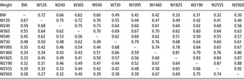
For both B-spline models, the correlations of animal permanent environmental effects decreased with increasing time interval between weights, with lower correlations being observed between weight at birth and weights after 730 days of age (Table 3). High animal permanent environmental correlation estimates were observed between weights from birth to 540 days of age and from 730 days of age until 8 years of age. Maternal permanent environmental correlation estimates between weight at birth and the other weights were of medium to high magnitude, and were higher between final ages. The maternal permanent environmental correlations estimated at the beginning of the study period differed from those reported by Baldi et al. (Reference Baldi, Alencar and Albuquerque2010), who observed negative correlations between weights from birth to 12 months of age, but close to unity between weights after 18 months of age.
Estimates of animal environment (above the diagonal) and maternal permanent environment (below the diagonal) correlations between weights from birth to adult age obtained for model BSQ5353.

BW = weight at birth.
W120, W240, W365, W540, W730, W1095, W1460, W1825, W2190, W2555 and W2920: weight at 120, 240, 365, 540, 730, 1095, 1460, 1825, 2190, 2555 and 2920 days of age, respectively.
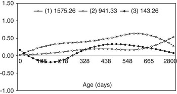
The three main eigenfunctions for direct additive genetic effect obtained with model BSQ5353 are shown in Figure 4. The three main eigenvalues of the coefficient matrix for direct additive genetic effects were responsible for 98.7% of the total direct additive genetic variation, with the first and second eigenvalue accounting for 59.2% of this variation. The first and second eigenfunctions for direct additive genetic effect were positive throughout the trajectory (Figure 4), indicating that selection based on these eigenfunctions will affect weights at all ages in the same direction. The third eigenfunction for direct additive genetic effect was negative from 60 to 300 days of age and positive during the remaining period. This sign change indicates that selection on this component will have opposite effects at the beginning and at the end of the trajectory. However, the possibility of genetic change because of selection on this eigenfunction is small as its eigenvalue was responsible for only 5.38% of additive genetic variance. Similar results have been reported by Baldi et al. (Reference Baldi, Alencar and Albuquerque2010) for weights of Canchim females from birth to 8 years of age.
Eigenfunctions (1, 2 and 3) estimated for direct additive genetic and their respective eigenvalues obtained for model BSQ5353 (order of fit of five for direct genetic and permanent environmental effects of the animal and of three for maternal genetic and permanent environmental effects, with five classes of residual variances).

Using weights of Angus females after 365 days of age, Meyer (Reference Meyer2005c) reported a wider fluctuation in the trajectory of the first two eigenfunctions for models with a larger number of segments or knots. According to Meyer (Reference Meyer2005b), eigenfunctions for direct additive genetic and direct permanent environmental effects obtained with RRMs using B-spline functions were more consistent or regular than those obtained with ordinary polynomials because of the better fit of B-splines.
RRMs using quadratic B-spline functions, as base functions, fitted the data similarly to Legendre polynomials, but higher number of parameters needed to be estimated with the former. However, the convergence was reached faster with B-spline functions than Legendre polynomials. According to Meyer (Reference Meyer2005b) and Misztal (Reference Misztal2006), applying spline functions the computational requirements are less than for corresponding analyses with the same number of coefficients, but using Legendre polynomial, because the matrices in the mixed model are sparser with spline functions.
In the data set studied, a model fitting quadratic B-splines, with four knots or three segments for direct genetic and animal permanent environmental effects and two knots for maternal genetic and permanent environmental effects, was a parsimonious model and was able to describe the covariance structure adequately.
Conclusions
A model fitting quadratic B-splines, with four knots or three segments for direct genetic and animal permanent environmental effects and two knots for maternal genetic and maternal permanent environmental effects, was the most adequate and parsimonious model to describe the covariance structure of the data. Despite the estimates of variance components and genetic parameter obtained by RRMs on Legendre polynomials, B-spline functions and multi-trait models were similar; RRMs on B-spline functions required less computational requirement and were time consuming. These aspects are very important to define an appropriate model for genetic evaluation in large scale.
Selection for higher weight, such as at young ages, should be performed taking into account an increase in mature cow weight. Particularly, this is important in most of Nellore beef cattle production systems, where the cow herd is maintained on range conditions. The likelihood to modify the growth curve in Nellore cattle in order to obtain animals with fast growth at young ages and moderate-to-low mature cow weight is restricted.
Acknowledgments
The authors thank the Fundação de Amparo à Pesquisa do Estado de São Paulo (FAPESP). We are indebted to the Associação Nacional de Criadores e Pesquisadores (ANCP) for the use of the data set.