The principle of hierarchy relies on the obedient compliance of agents at lower levels with the orders issued by their superiors. The problem of hierarchy arises because agents provide much of the information on which their superiors rely to monitor compliance and are able to exploit this information asymmetry in their own self-interest to seek a quiet life or skim off internal resources. This problem is magnified to the extent that the hierarchy in question does not fully control its external environment; this adds outside options to the agent's internal scope for disloyal behavior.
The Soviet command economy faced this problem in controlling the Soviet firm. Towards the end of the 1920s the Soviet state embarked on a mobilization drive that permanently altered the economy's microfoundations.1
Davies, “Changing Economic Systems.”
Controls on firm behavior arising from the market mechanism were replaced by administrative controls. The economy began to allocate a much higher proportion of the resources available to investment, and for some decades it also grew faster.
2 Bergson, Real National Income.
At the same time the Soviet firm did not suddenly become the obedient agent of centralized plans. Instead, the high-level ordering of resource allocation involved a running battle with the desire of agents at lower levels not to be mobilized but to pursue their own interests.
Economists have modeled these tendencies in a variety of ways. Researchers such as Joseph S. Berliner and Alec Nove quickly identified the information and incentive problems associated with administrative performance indicators.3
Berliner, Factory; and Nove, “Problem.”
Among these was the search for a “quiet life” that John Hicks had first associated with monopoly; Martin L. Weitzman developed this idea as a dynamic disincentive associated with the “ratchet” effect, and János Kornai generalized it as his famous “soft” budget constraint.
4 Hicks, “Annual Survey”; Weitzman, “Ratchet Principle”; and Kornai, Economics.
The interaction between the planned and market spheres also attracted attention. To some observers this naturally gave rise to the idea that the formal and informal sectors existed in a joint equilibrium.
5 Nuti, “Hidden and Repressed Inflation”; and Shleifer and Vishny, “Corruption.”
Others noted that, whereas corruption might grease the wheels of the command system in some respects, it could also undermine its legitimacy, implying that their joint equilibrium could only be temporary: eventually, one must drive out the other.
6 Grossman, “Second Economy,” “Notes,” and “Subverted Sovereignty.”
We begin our investigation from a historical, if stylized fact: the Soviet economy worked not unsuccessfully for a number of decades. This is not to say that it worked for the best, but it did provide full employment and, after a notably bad start in the thirties and forties, rising living standards. It did not harness the forces of self-interest particularly well, but it did harness them to some extent.
The literature does not provide a convincing explanation of how the planned economy made use of the self-interest of the producer. Existing models focus, as a rule, on the dysfunctions of the state-enterprise relationship and the incentives to inefficient or corrupt behavior. Such models are not wrong but they are incomplete in two senses. First, those that seek to capture the search for a quiet life and the toleration of inefficiency tend to downplay or exclude the pecuniary motivations that drove corruption and informal-economy behavior; symmetrically, those that focus one-sidedly on the preference for leisure do not account for preferences for money. Second, both classes of model are uninformative about the spurs to effort and improvement in the Soviet system, tending to view them as superimposed entirely from above. Such theoretical lacunae, moreover, limit our ability to understand the historical evolution of Soviet economic outcomes: what happened in the course of the 1970s, for example, that appears to have allowed the incentives that previously encouraged effort and productivity to slip increasingly out of alignment?
In this study we will provide a historically rooted model of the Soviet firm as an actor that pursued preferences for both leisure and liquidity, could exploit external opportunities for corruption, and also had to negotiate constraints imposed by the higher authority of the plan. In our model a plan-setter and an effort-setter fix the scale and uses of corrupt side payments simultaneously with effort, output, and prices. The firm, as effort-setter, exploits information asymmetries to invest in fake product innovations and cheat on price with the goal of obtaining a quiet life. The result is hidden inflation, with true real growth also being less than is claimed. The firm can additionally use corrupt revenues to siphon resources from consumer markets to make its life even easier. The plan-setter must find an optimal tautness. Increasing plan tension will make the firm try harder; there will be less private corruption because bribes will have to be recycled into meeting corporate goals. But corporate goals can be met as efficiently by pretending to satisfy the plan as by truly meeting it, and beyond a point there will be more pretense relative to production. On the other hand, if the plan is too lax, the firm simply takes the leisure and its employees pocket the bribes.
Our model is informed by the historical research that we and others have undertaken in the former Soviet archives since 1991. A new view of prices and monetary flows in the Soviet economy is at the core of this model. Standard models of Soviet pricing present the Soviet firm as a price-taker. The source of this stereotype is the official myth of the command system in which the center administered prices and imposed them on producers. Western economists had voiced longstanding empirical concerns about the stability of official prices, and especially how the enterprise might exploit product variations to free itself from price controls.7
These are surveyed by Harrison, “Soviet Industrial Production.”
This ought to have suggested that the idea of the Soviet firm as price-taker was oversimplified. But such concerns tended to be forgotten whenever economists were tempted to offer theoretical generalizations.
8 For example Ames, Soviet Economic Processes; Ericson, “Allocative Role” and “Second Economy”; Goldfeld and Quandt, “Budget Constraints” and “Output Targets”; Gregory and Stuart, Russian and Soviet Economic Structure; and Nove, “Problem.”
In contrast to these, we will start from the evidence-based proposition that the Soviet firm was a price maker: it held the initiative in the price-setting process through its control of the information that the center required to authorize pricing decisions, and exploited this advantage to set prices in a self-interested way.
The literature that we have already noted approached monetary flows in much the same spirit as it handled pricing. In theory, money was secondary. Firms' soft budget constraints were said to create seller's markets in which money was abundant and of low value; plans, rations, and the willingness to wait counted for more than money in determining resource entitlements.9
On the seller's market see Kornai, Economics.
The money stock itself was supposed to be strictly segregated into bank money for interfirm transactions and cash money for wage payments. The banks supplied money and credit to “follow” physical plans, and the planners monitored monetary flows mainly so as to practice “control by the ruble,” i.e., to detect departures from physical directives.
10 Gallik, Jesina, and Rapawy, Soviet Financial System; Garvy, Money; Nove, Soviet Economic System, pp. 243–44.
Given that firms could use money only for planned purposes, there would appear to have been little incentive for them to acquire additional holdings. In this view, money became an active influence on allocation only when it stimulated either entrepreneurship in the unofficial second economy, or corruption in the first, official one. In contrast we will show that Soviet managers displayed an active thirst for money and allocated considerable effort to getting it. When they got it they faced a choice: to pocket it or use it on the firm's behalf. With surprising frequency they allocated it to support the firm's objectives rather than their own.
In showing how this economy harnessed self-interest, we will draw a distinction between the agent's corruption and loyalty to her principal; we will show that corruption was not always driven by disloyal motives, and that managers made corrupt deals not only despite loyalty to the principal but because of it, in order to support loyal activity and enterprise. The phenomenon of the corrupt yet loyal manager is at the core of the mechanism that aligned self-interest with the plan.
Our findings address issues of interest to both economists and historians. For economists, we show that Soviet economic performance was affected not only by the level of corruption but also by its quality, that is, how corrupt incomes were used. This contributes to the literature on corruption and development. Corruption is said to flourish in conditions of authoritarian rule, which hinders accountability and promotes secrecy.11
Ehrlich and Lui, “Bureaucratic Corruption”; and Shleifer and Vishny, “Corruption.”
Corruption has been shown generally to reduce investment and growth.
12 However, the variation in growth rates across countries that are similarly corrupt and authoritarian is substantial and exceeds that among democracies.
13 Our model explains some of the heterogeneity: whether or not corruption is bad for growth depends on how corrupt incomes are used.
For historians we show how an instrument of policy, the level of plan “tension,” influenced the quality of Soviet corruption and thus Soviet economic performance. This contributes to the literature on the decay of the Soviet economy. Empirical studies have shown that the underlying trend in Soviet economic growth fell markedly during the 1970s; at the same time the scale of rent-seeking activities was increasing only modestly.14
On the trend in growth see Harrison, “Trends”; on rent-seeking see Kim, “Informal Economy Activities.”
This suggests that rising corruption was probably not the cause of the slowdown. Instead, we will suggest that the exogenous factor was a decline in plan tension that simultaneously determined the decline in growth and an adverse shift not in the
scale of corruption but in its
quality: namely, from loyal corruption to corruption that was disloyal.
The effects of “tension” in Soviet planning were first analyzed by Holland Hunter as a contribution to the theories of disequilibrium growth and development that were fashionable at that time.15
Hunter, “Optimal Tautness.”
The measurement of tension is a difficult problem. It cannot be approximated by reported plan failures, for example; we shall suggest that an increase in tension normally gave rise to an increase in cheating that concealed any shortfalls arising. For this reason evaluations of plan tension must rely principally on statements of belief and intention. A reduction of plan tension that, according to Gertrude Schroeder, apparently took place in the mid-1970s plays an important role in our story. It involved a moderate reduction in overall output growth and a near halving of investment growth; these were based, according to Schroeder, on “a determination to arrest the decline in the output/capital ratio, which had accelerated in industry in 1971–75; a conviction that lower growth targets, by easing the pressure on managers, would enable them to use resources more efficiently and to improve the quality of products; a belief that slower growth of investment would reduce plan tautness, slow accumulation of inventories, and substantially improve efficiency in the investment process.”
16 Gertrude Schroeder, “Slowdown,” p. 47.
Our investigation is organized as follows. We describe the historical limits on centralization of the Soviet command system. Specifically, Soviet managers exercised discretion over the accounting prices used in planning and prices and side payments that arose in decentralized contracting; they used this discretion to improve the ratio of reward to effort directly, and also to reduce effort indirectly by “siphoning” resources from the retail market. Then, we present a model of the Soviet firm in which there is no corruption and producers allocate effort subject to a plan target and a resource constraint. Following this, we look at the Soviet firm's use of corruption possibilities to relax its resource constraint through siphoning. At each point we consider the rationale for Soviet managers to engage in corruption and for planners to tolerate or restrain their behavior. Subsequently we test our model using historical data. Finally, we reconsider the historical scope for disloyal corruption.
THE LIMITS OF CENTRALIZATION
Standard models present the Soviet firm as a price-taker. According to Kornai, however, there were too many prices for the price-fixing authority to exercise this function effectively; instead, the authority “merely endorse[d] prices set by the producer” after a process of “vertical bureaucratic bargaining.”17
Kornai, Socialist System, p. 148.
If producers were free to set prices, how would they set them? Kornai neglected to go on to analyze the producer's pricing decision.
Addressing this gap in the literature, Andrei Shleifer and Robert W. Vishny proposed a model in which the socialist firm faces an incentive to cut both price and output relative to a market equilibrium in order to gain bribes. Given the price, the firm sets output to maximize corrupt side payments.18
Shleifer and Vishny, “Pervasive Shortages.”
This approach, which we will call the Shleifer-Vishny conjecture, sufficiently explains the phenomena of widespread shortages and corruption in socialist systems, yet does not sit well with the facts in other ways. First, Soviet firms worked continually for higher, not lower prices. Much detailed information is now available about how Soviet suppliers set industrial product prices; even a single example of a firm asking for a lower official price has yet to be found.
19 Harrison, “Prices”; and Harrison and Simonov, “Voenpriemka.”
Second, the Shleifer-Vishny conjecture is framed by an assumption that the planner could control prices perfectly if she wished, yet did not control quantities at all. The evidence that we will bring to bear indicates that planners controlled both prices and quantities, but imperfectly.
What was the significance of price-setting for the Soviet firm? According to the stereotype, the firm in the Soviet command system was managed by nonprice regulation of quantities. The Russian archives show us, however, that most targets that mattered in the Soviet economy were nominally defined. The most important control figures decided by the Politburo, the annual investment plan and the defense budget, including the plan for military procurements from industry, were fixed in rubles.20
Davies, “Making of Economic Policy,” pp. 64–66; Gregory, “Dictator's Orders,” pp. 17–18; and Harrison. “Prices” and “Providing for Defense,” pp. 99–100.
So were most supply quotas that were binding on production ministries and enterprises.
Centralized supply planning required a mechanism to prevent producers from satisfying ruble quotas by inflation rather than with real output. This mechanism was the system of plan prices. Supposedly the plan price of each product was fixed for the period of the plan. The anchor for each plan price was the “factory” price officially approved by the center in some past year, usually on the basis of reported actual direct costs plus an allowance for overheads. The motive for the producer to fulfill the plan then arose because her reward was formed by the degree of fulfillment based on reported real output multiplied by the plan price.
The authorities usually had enough information to prevent producers from adopting an openly inflated plan price for a given product, which would have broken explicit rules in observable ways. Producers could inflate the overall level of plan prices covertly, however, by exploiting gaps in planners' information about the product assortment and product quality.21
Harrison, “Prices” and “Soviet Industrial Production.”
Arbitrary variations in price/effort ratios across the assortment created one opportunity for this: by shifting the proportions of output towards products that were priced advantageously producers could push up the average level of plan prices although there was no change in any particular price. Another opportunity was represented by the modification of existing and introduction of new products. When products were upgraded the producer could claim a plan price increase that was supposedly based on the quality improvement, so that the price/quality ratio was kept stable. But the planners evaluated quality change on the basis of the producer's costs and the producer's justification, not the consumer's willingness to pay; the latter was meaningless anyway in a shortage economy. When new products were introduced subsequent to the base year for plan prices a benchmark plan price for that product had to be established from scratch, and planners based this on the actual unit costs that the producer now currently reported. Thus for both modified and new products the producer held the initiative in price-setting. In summary, producers used product change to exert upward pressure on the average level of plan prices; they inflated the nominal costs at which new and upgraded products were priced, and then they skewed the assortment towards these newer products. But the pressure was unseen and the inflation was hidden because it was always justified by quality claims.
Implicitly the inflationary pressure was not costless or limitless. To keep the pressure up producers had to play the game of product innovation. They had to modify their product lines continuously, whether the modifications were fundamental or phony, and whether or not they were truly useful to the purchaser; if not useful, Berliner called it “simulated” innovation.22
Berliner, Innovation Decision, pp. 375–80
They had to persuade the planners that the claimed modifications were useful regardless of the truth, bearing in mind that in the shortage economy the producers themselves could not know and the consumers might not care. The argumentation and the staging of innovation in support of it diverted company time and effort from production. From the firm's standpoint, however, an increase in the effort that concealed inflation lowered productive obligations on the firm by more than itself, and so yielded a net private gain up to a point. It is easy to think that the planners required disproportionately more argumentation to overlook each extra increment of hidden inflation, so that the concealment of inflation was characterized by diminishing returns.
Estimates of the scale of hidden inflation in Soviet industrial statistics vary with the methodologies used to evaluate quality and assortment. With regard to the early period of Soviet industrialization Harrison concluded that our best figure for hidden inflation in Soviet plan prices across industry from 1928 to 1955 lies between 150 and 200 percent; this includes a figure of 100 to 160 percent for machinery products in the period from 1937 to 1955.23
Harrison, “Soviet Industrial Production.”
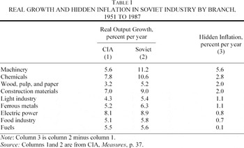
For the more recent period we can disaggregate hidden inflation across branches of industry from 1951 to 1987 as the excess of Soviet index numbers for the gross value of output at plan prices over CIA estimates that were designed specifically to strip the hidden inflation from the Soviet official figures. These are shown in
Table 1.
The CIA methodology has been exhaustively described in many publications.24
CIA, USSR, Measures, and Measuring Soviet GNP.
Although not above criticism it remains the best attempt at an extraordinarily difficult and complex task.
25 For example, Kontorovich, “Economists”; Kudrov, Sovetskaia ekonomika; and Maddison, “Measuring the Performance.”
According to the table, hidden inflation was highest in machinery at 5.6 percent annually, and almost nonexistent in fuels.
Soviet firms used their influence on price-setting not only to fool the planners but also to extract unplanned revenues from purchasers. The documentary evidence on this is plentiful and clear cut. Stalin's Politburo took the inflationary propensities of producers for granted; they determined and at times limited the annual investment plan, for example, believing that an ambitious plan fixed in rubles could be partly eroded in real terms by higher construction costs: the building industry would respond to a larger budget by raising costs above estimate prices.26
Davies, “Making of Economic Policy”; and Gregory, “Dictator's Orders.”
Records of bargains struck at lower levels provide further evidence that suppliers' preferences for product prices were always inflationary. In contrast to the firm portrayed by Shleifer and Vishny that gained from a lower price of output, it was typical for Soviet firms to try to push factory prices upward towards the market-clearing level.
The opportunity for inflation arose when suppliers and users negotiated the decentralized contracts that translated aggregate ministerial plans into firm-specific delivery obligations.27
On contracts see Belova, “Contract Enforcement”; Harrison and Simonov, “Voenpriemka”; and Kroll, “Decentralization.”
According to Eugenia Belova and Paul R. Gregory it suited planners and suppliers alike that centralized plans were issued in a highly aggregated form; this freed planners from responsibility for issuing specific assignments and gave suppliers freedom of action in deciding how to meet them.
28 Belova and Gregory, “Dictators.”
In the context of a seller's market the outcome was a ritual played out each year between ardent grooms (purchasers) and reluctant brides (suppliers) that became known as the annual “contracts campaign.”
Decentralized contracting allowed suppliers to use several stratagems to extract advantage from potential purchasers. As a result purchasers often paid for output above the rate set by officially established factory prices. In the defense industry, for example, Harrison and Simonov found unauthorized price increases in contracts for established products together with demands for contracts in which prices of new products were specified “provisionally” and subject to review in the light of actual costs, demands for illegal advance payments, and a variety of strategic actions that supported these demands: exaggeration of production costs, withholding of evidence concerning costs, refusal to permit the verification of costs, delaying coming to terms until well into the contract period, and refusal to come to an agreement at all unless concessions were made on the contract price.29
Harrison and Simonov, “Voenpriemka.”
Since Kornai much theorizing about command systems has started from the socialist firm's soft budget constraint.30
Its financial shortfalls would ultimately be made up from fiscal or quasi-fiscal sources. If so, why did firms invest so much effort in extracting liquidity from purchasers? The answer appears to be that managers set a high value on liquidity that was above the plan and, not having a planned use, could be used in a discretionary way.
What were the uses of discretionary cash? Managers behaved corruptly not just for private embezzlement as Shleifer and Vishny supposed, but also to help the enterprise fulfill its plan.31
Belova, “Economic Crime.”
With cash at their disposal they could finance side payments to their own workers and to unofficial
tolkachi (supply agents), and also “siphon” needed but unplanned resources away from the retail market. Here we focus on siphoning.
The idea of firms' siphoning from the retail market is not as strange as may appear at first sight. Of course the retail market did not supply firms with specialized producer goods such as metal-cutting machine tools, road or rail trucks, steel ingots, or nonferrous castings. But many general-purpose goods and services that were planned for consumer supply could also be used in production: transport services, fuel and power supplies, information and communication technology, light automobiles and parts, electrical components and fittings, building materials, furniture, and office supplies. These were the commodities over which firms competed with households in the retail market.
Siphoning plays an essential role in the theory of the soft budget constraint. Specifically it solves the riddle posed by Shleifer and Vishny: “In Kornai's model,” they wrote, “it is not so much that goods are underpriced, but that the income of the buyers is effectively infinite. This model may be appropriate for some intermediate goods. But households face hard budget constraints, and therefore the systematic shortages of many consumer goods remain a puzzle.”32
Shleifer and Vishny, “Pervasive Shortages.”
In fact a soft budget constraint for firms could result in shortages for consumers if firms' demand for inputs spilled over into retail outlets.
This idea had long been floated in the Sovietological literature.33
Birman, “Financial Crisis”; Kaser, ”Economy”; and Kornai, Economics.
However, the existence of siphoning remained conjectural, especially as it required firms to be able to mobilize unauthorized purchasing power. Even if siphoning occurred its scale and significance remained doubtful. If it was significant, it was unclear why the authorities tolerated it.
More recently Mathias Dewatripont, Eric Maskin, Yingyi Qian, and Kim provided the pieces necessary to solve this puzzle. Dewatripont and Maskin showed how centralization of credit leads to a soft budget constraint in the context of sunk costs and contract renegotiation.34
Dewatripont and Maskin, “Credit.”
Qian showed that when state-owned enterprises compete with households for goods that may be used in both consumption and production, prices below the clearing level may improve efficiency by allowing household consumption to crowd out some bad projects that would otherwise proceed.
35 Finally, Kim showed from postwar archival records that Soviet firms and budgetary organizations did engage in siphoning, that their demand spilled over into the retail market through unauthorized channels in addition to some that were officially sanctioned, and that siphoning made a substantial contribution to repressed inflation and a growing monetary overhang in the Soviet retail market.
36 Kim found that the siphoning of consumer goods was prevalent in the Soviet era. Enterprises' supposedly “passive” money was used to purchase consumer goods without official authorization. Archival data of the Soviet family budget surveys from 1969 to 1990 show that the consumer goods purchased using enterprises' “passive” money averaged 21.3 percent of total retail turnover of consumer goods. The scale of siphoning tended to rise over the period, from 16 percent of total retail turnover of consumer goods in 1969 to 23 percent and 26 percent in 1980 and 1989 respectively. However, this does not mean that siphoning was absent in earlier periods, and its most important statistical trace can be found in all periods of the history of the command system. This was the excess of household spending over income found whenever government statisticians computed the balance.37
Hanson, Consumer; Holzman, “Soviet Inflationary Pressures.”
The excess arose because unauthorized institutional purchases in the retail market were hidden in the totals for household consumption.
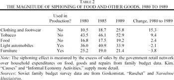
The pattern of siphoning was likely to reflect management objectives. When faced with ambitious plan targets the manager was less likely to convert discretionary cash into consumption and more likely to plough it back into production. When planning tension was slackened, however, consumer objectives could return to the fore. On this basis one might predict that a relaxation of plan tautness would increase the siphoning of food and consumer goods relative to that of goods that could also be used in production. Table 2 reports the extent of siphoning across types of commodities classified according to their potential for intermediate use, in 1980, 1985, and 1989; over these years plan tension fell, period by period. The table shows clearly that, whereas the siphoning of consumer goods increased, that of general purpose commodities such as furniture and light automobiles that could also be used in production stagnated or declined.
Cash was the instrument of siphoning, and siphoning should be considered an established fact, but the full range of mechanisms through which Soviet firms could mobilize cash or freely encash bank deposits is not completely clear. The Soviet financial system was designed to separate monetary flows between two distinct circuits, one for anonymous cash and one for traceable noncash bank credits.38
Gallik, Jesina, and Rapawy, Soviet Financial System; and Garvy, Money.
In theory budgetary and state-owned enterprises were allowed to use only noncash credits in transactions with other organizations; cash was restricted to a parallel circuit of household transactions.
From the start, the realities of the financial system departed from this design. Budget constraints were softened and credit conditions became chaotic.39
Gregory and Tikhonov, “Central Planning.”
It was widely believed that Soviet enterprises had more cash in aggregate than the plan had authorized.
40 Birman, “Financial Crisis”; and Grossman, “Inflationary, Political, and Social Implications.”
This suggests that enterprises gained the above-plan liquidity used for siphoning not only from each other in side payments but also from breaking the central bank's restrictions on cashing bank deposits.
The evidence on this is somewhat mixed.41
For competing views compare Gregory, Restructuring the Soviet Economic Bureaucracy; Gregory and Tikhonov, “Central Planning”; Granick, Job Rights; Holzman, “Soviet Inflationary Pressures”; Lushin, “Material'no-finansovaia sbalansirovannost”'; Treml and Alexeev, “Growth”; Woodruff, Money; and Gregory and Tikhonov, “Central Planning.”
In our own theorizing we assume that the firm cheated the planner through hidden inflation and extracted hidden revenues from the customer, and did not cheat the central bank. This assumption will not significantly affect our conclusions. A model of the macroeconomic equilibrium, however, would need to incorporate the government's budget constraint and the balance sheet of the central bank so as to account for overall liquidity growth.
PLAN-SETTING AND EFFORT-SETTING
In this section we develop a framework in which the firm cheats the planner and behaves opportunistically but not corruptly. At this point it may be asked why the firm did not try to corrupt the planner. The answer appears to be that Stalin and his successors deliberately separated planners from management responsibility and kept their numbers small to ensure their loyalty.42
Belova and Gregory, “Dictators”; and Gregory, Restructuring the Soviet Economic Bureaucracy.
In the Soviet command economy planners aimed to monitor real output for each firm in each period. The firm's target was its real gross output expressed in plan rubles; this was calculated as a quantity vector q* multiplied by a vector of official prices p−1 that applied in the previous base period. In practice, however, planners could not effectively compel firms to fulfill the plan at base-period prices. When products were changing, planners tried to limit changes in product-unit prices to those that left the level of prices per unit of characteristics unchanged. They could prohibit open inflation, but continuous alterations in the product assortment and product characteristics left planners unable to detect the hidden inflation associated with simulated product innovation. In short, we define hidden inflation in relation to planners, not consumers who knew what prices they faced. Inflation was concealed and the planners were fooled when the firm pushed up product-unit prices faster than the value to the user of the improvement in product characteristics, or when product-unit prices remained constant despite unreported worsening of product quality.
As a result the planners had to be satisfied ex post with any real output vector q that, combined with a new current price vector p set by firms and subject to planners' limited scrutiny of price alterations, matched the ruble total set by them ex ante. But it is simpler if we treat the firm's average price and quantity as scalars.
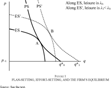
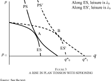
This equation is represented in Figure 1 by the unit-elastic PS or plan-setting curve, which required q = q* when p = p−1 and there was no hidden inflation: the vertical axis in the figure represents the true level of the official price, including the inflation that the planners failed to detect, and the PS curve shows the rate at which producers could trade hidden inflation for real output while continuing to satisfy the plan. Similarly, the horizontal axis measures not the output that was officially reported but true real output, corrected for the exaggerated claims that producers made for the quality of their products in order to fool the plan-setter.
FIGURE 1 PLAN-SETTING, EFFORT-SETTING, AND THE FIRM'S EQUILIBRIUM
We represent what happened when the planner increased tension by shifting the PS curve rightward shift from q*0 to q*1 and to PS′, requiring the firm to achieve some higher level of true real output for given concealed inflation so as to satisfy the plan.
From the firm's point of view output was costly, but so was the concealment of inflation, because both required the exertion of effort. Think of the firm's utility as based on its members' wage income w and leisure λ
where uw and uλ are the first derivatives of u with respect to w and λ respectively, uww and uλλ are the second derivatives of u with respect to w and λ respectively, uwλ is the cross-derivative of u with respect to w and λ and uλw is the cross-derivative of u with respect to λ and w; these definitions of first and second derivatives are retained in other equations below. The wage could assume two values: a fixed return w =
if the firm satisfied the planners' target and otherwise nothing, w = 0. This is the classical Soviet incentive scheme in a simplified form.
43 Berliner, “Informal Organization.”
We assume that leisure and income interact, so the firm required at least some of both. Berliner first noted the significance of a “quiet life” for the Soviet enterprise. In order to have any income at all the firm had first to satisfy the output target, and then it could also maximize leisure. The firm maximized leisure subject to a resource constraint that we shall treat initially as hard
where e is productive effort, i is the effort required to simulate innovation and so conceal inflation, and the firm's initial time endowment is normalized to 1.
Finally, there were two technologies, one for the production of output a and one for the concealment of inflation x. Production required effort to be combined with capital k, but for now we will treat capital as an exogenous resource. Inflation concealment required effort alone. In both activities, returns to effort diminished
Then, for any given level of overall effort that it chose to set, the firm faced a feasible set of combinations of real output and hidden inflation that was concave to the origin (proposition 1: for propositions, proofs, and a list of symbols see the Technical Appendix).
We call this the ES or effort-setting curve. For each firm and for every production and concealment technology there was a family of ES curves, one for each feasible level of effort. In Figure 1 the ES curve illustrates the combinations of real output and hidden inflation that were feasible given effort level 1 − λ0. As the firm set its effort level higher, say to 1 − λ1, the ES curve expanded in all directions, say to ES′ (proposition 2).
Facing a given plan the firm's problem was to allocate effort between production and inflation concealment so that the plan was fulfilled and effort was set at a minimum. In Figure 1 this point is found at A where the plan-setter's line PS is tangential to the lowest available effort-setter's line, ES corresponding with leisure, λ0, and it sets the equilibrium values of real output and hidden inflation simultaneously. The firm could also have satisfied the planner with more real output and less hidden inflation, or with less real output and more hidden inflation, but either of these would have required the firm to shift its effort curve outward and cost more effort, say 1 –λ1 for ES′.
The figure also shows what happens when the planner increased tension, right-shifting PS from q*0 to q*1. To continue to satisfy the plan the firm had to move to the higher ES′ curve defined by λ1. At the new equilibrium B there would be less leisure and more real output, but diminishing returns to productive effort made it inefficient for the firm to meet the higher plan only by increasing real output. Some of the extra effort would go into fooling the planners. In equilibrium real output rose by less than the change in q* and there was also more hidden inflation than before.
Simple extensions of the model suggest conditions under which the command system may break down. The system's directors had to steer a course between excessive liberalism and excessive harshness. First, suppose the plan was set at a level that could not be fulfilled with any combination of real output and hidden inflation given the firm's hard resource constraint. Producers would then prefer zero effort, reward, and utility to the welfare loss resulting from trying and failing to fulfill the plan; there would be no hidden inflation, but output would collapse to the origin. The turmoil induced by Stalin's Great Breakthrough and Mao's Great Leap Forward comes to mind. Second, if prices were fully liberalized within the command system producers would use their new freedom to climb the PS curve, raising prices without limit and cutting real output to a minimum. This time one thinks of the Soviet economic collapse at the end of the 1980s.44
LOYAL CORRUPTION
So far we have assumed that the enterprise was subject to a hard resource constraint. In fact, although resources for production and consumption were constrained in total for the economy as a whole, the resource constraint on the individual firm could be softened by collecting corrupt revenues and recycling them through siphoning, and so adding outside resources intended for consumption to the production inputs officially allocated to the enterprise. Our attempt to capture the outcome will resemble the Shleifer-Vishny story of the bribe in some respects, but in our initial model the bribe is collected in order to fulfill the plan, not to line pockets. The result is that, with plan-setting unchanged, real output rises while both hidden inflation and insider effort fall; the inflation experienced by consumers also rises, however.
Subsequently we will examine the implications of bribe-taking for personal enrichment, or embezzlement. However, unlike Vishny and Shleifer we do not regard embezzlement as the general case. We will draw a distinction between corruption and disloyalty. All managers were potentially corrupt, but only disloyal managers used the proceeds for personal enrichment; loyal managers used them to fulfill the plan. Such loyalty was rational. In the vertical administrative hierarchy managers were expected to invest in loyalty both upwards and downwards. Managers showed loyalty to their superiors for the sake of their careers: to be promoted, they needed a record of plan fulfillment. But this record also relied on meeting the needs of inferiors and maintaining their cooperation, so managers also had to show loyalty to the workforce. Consistent disloyalty in either direction, upward or downward, prejudiced career aspirations. Because these loyalties could come into conflict, successful management involved complex balancing. Of course, disloyal corruption that was for personal enrichment also brought a return, but the value of the return was less than might be thought as cash was often hard to spend on personal consumption; this was both because of the seller's market and also because of the need to avoid attracting attention.
Belova reports what she calls the “honest” manager's dilemma, but in this system no one was completely honest, so we will call it the dilemma of the loyal manager.45
Belova, “Contract Enforcement.”
To fulfill the plan, the manager had to compete for scarce supplies that the planners forgot, or promised but did not deliver. To compete, she had to pay. Payments went to sideline suppliers of deficit commodities, unofficial purchasing agents, and workers for the extra effort required to make bricks without straw. We will analyze siphoning: so as to augment their own productive stocks, firms entered the retail market as purchasers of commodities intended for sale to households for personal consumption. For this purpose the loyal manager had to acquire discretionary liquidity by creating revenues that were hidden from the planners. She got the liquidity from her own purchasers by securing an above-list price, or advance payment, or bribe, but, in distinction from the Shleifer-Vishny story, the bribe was credited to the firm's account.
First, rewrite the firm's production function from equation 4, adding Δk to represent the availability of an outside resource that substitutes perfectly for the firm's inside stocks of fixed and working capital:
In order to get hold of Δk the firm requires hidden revenue for discretionary use in the secondary market where commodities are traded that are of potential intermediate use. This hidden revenue must be over and above the liquidity officially allocated in the firm's financial plan. The firm extracts this hidden revenue in advance from consumers in its own product market: the hidden revenue gathered in the previous period is used to add to the firm's real resources in the current period. The coexistence of regulated and market-clearing prices in shortage economies is a well established historical fact, which can be rationalized in economic theory by reference to consumers' heterogeneous valuations of time versus money.46
Kim, “Soviet Household Saving Function.”
Suppose the firm can capture some proportion of the gap between the regulated and market-clearing price in the form of an advance payment, side payment, or mark-up over its officially listed product price without being detected; for simplicity we can set this proportion at 100 percent without affecting core results. The firm uses its hidden revenue as discretionary purchasing power in the secondary market. How will siphoning affect the ES curve? The result will be a new ES′ curve that is still concave (proposition 3) but right-shifted by comparison with the no-siphoning case (proposition 4). For a baseline illustration, consider how the structure of the firm's incentives is changed in what we will call the “single-transaction” case. The single transaction begins in period −1 when the firm sells a commodity in return for a side-payment and recycles it through siphoning to acquire Δk. The same transaction ends in period 0 when the firm uses Δk to satisfy the plan-setter and augment its utility, but the firm makes no provision for repeated siphoning of resources to be used in period 1. Thus the single transaction takes two periods to complete, but the only decision we analyze is the firm's optimization within the current period.
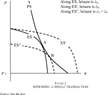
This case is illustrated in Figure 2. Initially the firm was subject to a hard resource constraint. Given plan-setting, the firm was in equilibrium with the solid effort-setting curve ES at point A; leisure is λ0, say. Softening its resource constraint through siphoning enabled the firm to produce more for given hidden inflation and given effort. The dashed ES′ curve illustrates the production-augmenting effect of siphoning with leisure held still at λ0. Because ES′ lay partly outside the firm's PS curve, it was not efficient for the firm to maintain effort at this level. As long as plan-setting remained unchanged, the firm would prefer to cut effort to a lower level, say 1 − λ1, yielding an ES″ line that, with augmented productive capital, was skewed downward and rightward from the no-siphoning ES curve and touched PS at B, a point showing more real output and less hidden inflation.
FIGURE 2 SIPHONING: A SINGLE TRANSACTION
In short, behaving corruptly to soften her resource constraint helped the loyal manager to fulfill the plan with less effort, less hidden inflation, and more true real output than would have been possible otherwise. This result suggests that not only the firm gained; there was also less fooling of the planners, for whom there was a clear rationale to turn a blind eye to the rule-breaking involved because, in the outcome, the plan was fulfilled more honestly.
The welfare implications are ambiguous, however. Consumers would have been better off in the current period in terms of real consumption because real output had increased. As long as production finished at the end of the current period we can assume that all goods produced currently were consumed. But it is not clear that this period's consumption would have risen by enough to compensate for the consumption lost in the last period by being recycled back into production. This depends on the efficiency with which the firm captured hidden revenues and converted them into additional inputs, and on the firm's initial endowment; a firm that started capital-poor would make more productive use of siphoning.
For consumers subject to a cash constraint, the effect of siphoning on prices must also be taken into account. Consumers would have paid less for supplies in the current period because of less hidden inflation, but in the previous period some of them would have paid more for supplies because of a combination of higher free market prices and covert side payments.
Next, we show that the rise in plan tension could have induced enterprises to use siphoned resources for higher output rather than effort reduction; thus, consumer welfare was more likely to improve when siphoning was combined with a rise in plan tension.
Figure 3 shows a possible outcome. The firm's capacity gain from siphoning, controlling for effort, is the shift from ES to ES′. The increase in plan tension is the shift from q*0 to q*1 and from PS to PS′. In the case of a corrupt but loyal manager, this increase would exactly capture the firm's additional resources, moving its equilibrium from A to B. At B, effort is the same as at A. Thus, the increase in plan tension has prevented the firm from using corrupt gains to augment its leisure. Real output has risen, though less than in proportion to the rise in plan tension, and there is also more hidden inflation.
FIGURE 3 A RISE IN PLAN TENSION WITH SIPHONING
REPEATED SIPHONING
The Shleifer-Vishny model prompts the question whether a corrupt supplier could gain by restricting output. To address this question we go beyond the case of a single transaction. In the single-transaction case the value of side payments was fixed beforehand. Effort was not optimized to supply the market in such a way as to secure further side payments as a basis for repeated siphoning. Side-payments depended on the gap between the market-clearing price and the official price. When siphoning is continuous this gap can be determined simultaneously with the effort-setting decision because market-clearing and official prices both decline, but at differing rates, as real output rises. The official price varies inversely with output along the PS curve, the latter being unit price-elastic. The market-clearing price varies inversely with output along the demand curve as the balance in the market shifts from seller to buyer. We assume a market demand curve as follows, linear for the sake of illustration
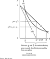
Consider how the firm's hidden revenues would have changed as real output increased. We observe that the firm's hidden revenues depended on the relative elasticities of the PS and market demand curves. The PS curve, which could also be termed the planner's demand curve, determined open revenues but was unit-elastic: the firm had to achieve a fixed total planned revenue, which in this context became a lump-sum tax. Assume for simplicity that the firm succeeded in extracting all the side payments that the market could bear; then, the market demand curve determined the firm's total revenue. Being downward-sloping and linear, its elasticity fell as output rose. Where the elasticity of the market demand curve equaled unity, the firm's total revenue was maximized and, because its planned revenues were a lump sum, its net hidden revenues were also maximized.
In Figure 4 the siphoning firm operates in the “shortage” region between
and
where the market-clearing price exceeds the official price; it is also a necessary condition that both prices exceed the baseline plan price p−1. In this region, assuming that the firm is able to extract the market price on its total output, the gap between the PS and D (market-demand) curves represents the firm's hidden revenue per unit of output. It maximizes its total hidden revenues midway between
and
, which is also the point where marginal revenue becomes zero and the marginal revenue curve, drawn with slope −1/2π, meets the quantity axis (drawn here at p = 0, not p = p−1). On either side of this point hidden revenues diminish, falling to zero at
and
.
How is the ES curve affected when side payments are endogenous? The result is a bubble on the ES curve in the region between
and
. In the single-transaction case (Figure 2) the whole ES curve was right-shifted in favor of higher real output. When siphoning is repeated the displacement of the ES surface is limited to the shortage region and is upward and variable, reaching its maximum extent at the level of output where hidden revenues are maximized. This drift is determined by the PS and D curves alone, and there is therefore a bubble on each member of the family of ES curves in the region between
and
.
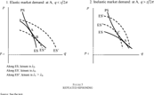
How does repeated siphoning influence the PS-ES equilibrium? For simplicity we assume that the relationship between hidden revenues and resources siphoned becomes linear with constant returns. Siphoning is maximized where hidden revenues are maximized. Thus, over the output range where the linear market demand curve is more elastic than the PS curve and hidden revenues are increasing, the siphoning bubble makes the ES′ curve flatter, and conversely. Under continuous siphoning, therefore, the downward slope of the ES′ curve varies directly with that of the market demand curve.
If ES′ was made flatter then the siphoning equilibrium tended to shift in favor of higher output; conversely, if steeper the siphoning equilibrium would have tended towards higher hidden inflation (proposition 5). The two cases are illustrated in Figure 5. In each panel point A marks the no-siphoning equilibrium. On the left, Panel 1 shows the case where, with a low value of π, the market demand curve was still elastic at the no-siphoning equilibrium; then for given output the ES′ curve would become flatter, and the siphoning equilibrium tended to shift towards higher output. Intuitively, the firm that faced elastic market demand lost hidden revenue by restricting output. Instead, up to a point dictated by diminishing returns to effort and liquidity the firm produced extra output, took the extra hidden revenue, and used it to buy extra inputs. For insider effort set at 1 − λ0 the ES curve expanded to ES′. This effort was above the efficient level, so the firm cut effort to the lower ES″ where effort was 1 − λ1 and λ1 > λ0. The outcome was an equilibrium at B with less hidden inflation and more real output.
FIGURE 5 REPEATED SIPHONING
The welfare implications of continuous siphoning for consumers in the case of a relatively flat market demand curve are again ambiguous. Consumers could enjoy higher consumption, as in the single transaction case, but only if the volume of true real output increased by enough to compensate for the loss of consumption due to continuous siphoning. As for the aggregate price level that consumers faced, this could go up or down depending upon three factors: the decrease in hidden inflation compared to the no-siphoning case, the excess of the market-clearing price over the official price, and the proportion of consumers paying the market-clearing price.
Panel 2, on the right of Figure 5, shows the converse case. With a higher value of π the market demand curve was already inelastic at the no-siphoning equilibrium; then for given output the ES′ curve would be made steeper, and the siphoning equilibrium tended towards higher concealed inflation. The firm facing inelastic demand could raise hidden revenue from side payments by restricting output. This case is more consonant with the stylized facts of a shortage economy proposed by Shleifer and Vishny. But in our case the firm, while restricting output to increase hidden revenues, still had to satisfy the planners. It did so by diverting the effort released by external resources siphoned from the secondary market to hiding inflation rather than producing output. The outcome at C was more hidden inflation and less real output.
Further, successive increases in plan tension would no longer necessarily shift the firm's equilibrium towards higher levels of real output. This is because the firm's point of maximum hidden revenues was fixed by the market demand curve. In Figure 5, other things being equal, a rise in plan tension shifted the firm's no-siphoning equilibrium to the right, and at the same time the probability rose that the no-siphoning equilibrium would drift to the right of the point where the firm's hidden revenues were maximized. At this point the firm might rationally prefer to curtail any further increase in real output that would drive down hidden revenues and reduce siphoned resources. This placed an ultimate limit on the ability of the planner to raise plan tension so as to maintain productive effort and raise real output when siphoning was repeated.
Finally, when market demand was inelastic the implications of continuous siphoning for consumer welfare were clearly negative: consumers became worse off in terms of both consumption and the price level. Resources siphoned away from consumption resulted in lower output; not only did the official price increase but, in addition, some consumers also had to pay the higher market-clearing price. This aspect of our model yields two testable predictions.
TWO TESTS
Prediction 1. Other things being equal, hidden inflation should have been inversely correlated with the price elasticity of market demand at the firm level. Specifically, we can rewrite equation 5 for the case of repeated siphoning in the form
where the dependent variable is the inflation concealed by the jth firm, ηj is the elasticity of market demand for the firm's product, and Xj is a vector of industry-level fixed effects that determine the firm's private effort costs of operating the concealment technology.
Prediction 2. Other things being equal, the change in hidden inflation associated with a given change in plan tension over time should have varied directly with the firm-level price elasticity of market demand. Specifically, we showed that the downward slope of the ES′ curve would vary directly with that of the market demand curve. The flatter was the ES′ bubble at the siphoning equilibrium, the more a given reduction in plan tension was likely to reduce hidden inflation.
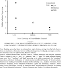
Here are three problems: to observe inflation that has been hidden, to identify the elasticity of the firm's market demand curve, and to control for fixed effects across industries. In Table 1 we measured hidden inflation across nine branches of industry over the period 1951 to 1987 as the excess of Soviet volume index numbers over CIA estimates that were designed to strip hidden inflation from the Soviet official figures. These are the figures used to measure hidden inflation along the vertical axis of Figure 6.
FIGURE 6 HIDDEN INFLATION, MARKET DEMAND ELASTICITY, AND INFLATION CONCEALMENT COST IN SOVIET INDUSTRY BY BRANCH, 1951 TO 1987
For the elasticity of demand and the effort cost of inflation concealment across industries we provide some informed guesswork. We set the effort cost of inflation concealment low in machinery where rapid product innovation was intrinsic to technological change throughout the economy, and in light industry where consumers placed a premium on novelty, high in electric power, ferrous metals, and fuels where standardization and product homogeneity were easily monitored and at a premium, and at an intermediate level in other branches (for further support see our note to Figure 6).
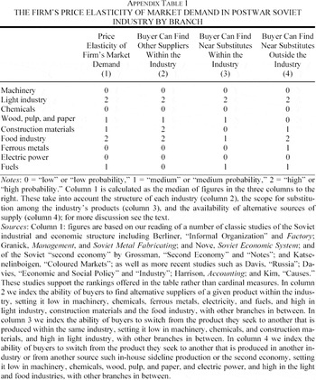
As for elasticities, we observe the factors underlying the firm's elasticity of demand in three different ways (for further support see the Data Appendix). First, the structure of each industry determined the buyer's ability to choose among alternative suppliers within the industry; the buyer could shop around among official and unofficial suppliers to a varying extent, and the opportunity for this arose in the contract stage of plan implementation that has already been described. Second, the buyer had more or less scope to substitute within each industry's range of products. Third, the frustrated buyer had varying choices among the substitutes for each industry's products available from other industries, unofficial markets in the “second” economy, or the buyer's own in-house sideline production. We take the median of the three resulting indexes to estimate the relative elasticity of the demand curve facing the individual firm in each industry; in Figure 6 we classify it as low, medium, or high along the horizontal axis. We conclude that price elasticity was high in the light and food industries, low in machinery, chemicals, and electric power, and medium in other branches.
Figure 6 shows that, taking the postwar period as a whole and controlling for concealment costs, hidden inflation did rise across industries as firm-level demand became more inelastic. This conforms to our first prediction.
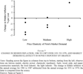
To capture the effects of a change in plan tension we measure the change in hidden inflation across industries comparing the low-tension 1980s with the higher-tension 1950s and 1960s. As Figure 7 would suggest, the annual rate of hidden inflation in industry as a whole fell over this period by 1 percentage point, a result that might surprise those who see Soviet postwar economic history in terms only of rising disorder, but is entirely consistent with our framework. A stronger test is the pattern of decline across industries. Figure 7 shows that the change in hidden inflation associated with the fall in plan tension did vary directly with the price elasticity of market demand. This conforms to our second prediction.
FIGURE 7 CHANGE IN HIDDEN INFLATION, 1980 TO 1987 OVER 1951 TO 1970, AND MARKET DEMAND ELASTICITY IN SOVIET INDUSTRY BY BRANCH
To summarize: an increase in plan tension would reduce the scope for both corruption and siphoning. This was evident from Figure 4: the firm may extract a net surplus of hidden revenues only when market demand exceeds planned revenues. An increase in the firm's planned output reduces the gap between the two and so limits the firm's corruption possibilities. When siphoning was repeated and firms responded to the resulting possibilities with adverse effects on real output, regardless of whether managers were loyal or disloyal, tautening the plan was a mechanism to limit corruption and corruption-oriented behavior. Conversely, reducing plan tension expanded the scope for both corruption and disloyalty.
DISLOYALTY
In this economy all managers were self-interested, and all managers were corruptible, but the manager we have described so far remained loyal. By accepting illegal side-payments and disbursing them via the siphoning mechanism, she fulfilled the plan while saving effort. This manager was therefore loyal simultaneously to superiors and to the workforce.
Not all managers were loyal, however. From our present knowledge we cannot easily work out what was the balance of loyal versus disloyal behavior at any given point. Even at the time, principals themselves could not easily distinguish the unofficial deals that agents made to fulfill the plan from those that lined their pockets. From the evidence of illegal dealing recorded by the courts and extra-judicial investigative organs of the Stalin era, Eugenia Belova has shown that, faced with the same facts of illegal dealing, officials could disagree over whether to see a criminal act or a loyal one.47
Belova, “Economic Crime.”
A recent study of the last Soviet-era anticorruption drive suggests that disloyal agents would always claim loyal motivation, and sometimes the investigators themselves did not want to know because they had a private or political agenda of their own.
48 Duhamel, “Last Campaign.”
Decades after the event we are unlikely to be able to determine whether loyal acts outweighed disloyal ones in some numerical way.
In our framework the absolute quality of Soviet corruption is not what matters. What is important is its relative quality: whether it tended to be more aligned to the aims of the Soviet state than would be normal in market economies, and whether the relaxation of Soviet plan discipline in the 1970s caused it to become less aligned.
Here we consider briefly the implications of disloyalty. A manager might choose to be either completely or partly disloyal. A completely disloyal manager embezzled all side payments for personal enrichment, so there would have been no siphoning and the firm's resource constraint would remain hard. The fact of widespread siphoning implies that complete disloyalty was not typical. We suggest that in practice the scope for managerial disloyalty was limited by workers' and planners' responses.
To support this we specify the distribution of information about disloyal behavior by managers as follows. Suppose that information about particular disloyal acts was only available to other agents within the firm. Above the firm, there was information only about the general incidence of corruption possibilities. If the manager was disloyal, the workers knew, but the planners could only suspect.
With respect to the workforce the manager with a disloyal propensity faced the following problem. She could sufficiently maintain her reputation upward by fulfilling the plan. But to fulfill the plan the manager needed the cooperation of the workers, who would have knowledge of her disloyalty. The workers might threaten to withhold effort, or alternatively to disclose her wrong-doing, to induce her to share the gains from corruption. In principle this sharing might be done in two ways. First, the corrupt manager might distribute part of the bribe income directly to the workforce in cash, but on our understanding of the context and evidence this was detectable, therefore dangerous, and seldom done. Instead, managers bought cooperation by transforming cash rents into additional resources through siphoning and sharing the gain with the workers in the form of leisure. As a result, for a given plan, insiders' effort fell. In this form rent-sharing was less visible to higher-level audit or even looked “good.” In short, complete disloyalty was not feasible: self-interested managers were always at least partly loyal.
Consider the problem of the same disloyal manager in relation to plan-setters. Plan-setters did not know firms' intrinsic capacity, or the extent of disloyalty, or the extent to which bribes were recycled into siphoning. They knew there was corruption, that siphoning might occur as a result, that siphoning enlarged firms' capacity, and that even disloyal managers would rationally choose to recycle some bribes into siphoning. They knew therefore that when siphoning arose the effort level and the utilization of capacity would tend to fall with an unchanged plan. Thus they would rationally respond to information about increased corruption possibilities by tautening the plan.
The disloyal manager wished to pocket the gain herself. But she still had to conserve her reputation with plan-setters by fulfilling the plan. Because the planners' knowledge of corruption possibilities led them to set a higher plan, the disloyal manager now had to get the workers to work harder. For this she needed the workers' cooperation, and this forced her to share the proceeds of corruption with the workers by engaging in siphoning to enlarge capacity and limit effort. In short, when managers were corrupt, raising plan tension was a mechanism to limit disloyalty. But the converse was also the case: reducing plan tension could promote embezzlement by corrupt managers. This result establishes a clear mechanism that links the spread of disloyal corruption through the Soviet economy in the 1970s with the simultaneous reduction of growth targets.49
On corruption see again Grossman, “Second Economy” and “Notes”; on growth targets, Schroeder, “Slowdown.”
CONCLUSIONS
We have analyzed the Soviet firm as a price-setter that interacted with a plan-setter and an external market to determine real output, hidden inflation, corruption, and siphoning simultaneously. In the case of a single siphoning transaction, we have found a clear rationale for Soviet planners to tolerate corruption and siphoning. Managers allocated resources that were gained corruptly to produce more real output with less hidden inflation and fulfill the plan more honestly as a result. Self-interested managers, however corrupt, always remained at least partly loyal to the goals of planners and workers. Moreover, by increasing plan tension, planners could induce disloyal managers to recycle more hidden revenues into production. Thus, tautening the plan limited managerial disloyalty. The implications for the welfare of Soviet consumers are ambiguous, however.
We have qualified these results for the case of siphoning repeated in continuous time. In this case higher real output was not the invariable consequence. When siphoning was continuous, the consequences for the welfare of consumers were less likely to be positive. But raising plan tension appears to have remained an effective mechanism for limiting the scope for corruption and adverse corruption-oriented behavior.
Our findings also reflect on the relationship between Soviet corruption and shortage. On the basis of the evidence we reject the Shleifer-Vishny conjecture that the shortage economy was organized with the intention of distributing bribes to individuals. Rather, the shortage economy had a by-product, corruption, that planners tolerated for their own purposes. Corruption did create scope for disloyal agents to line their pockets, but it could also help to align the objectives of suppliers with those of planners. Planners could influence the scope for both corruption and disloyalty by manipulating the degree of plan tension; it seems likely that reductions in Soviet plan tension in the 1970s contributed to the privatization of corruption rents in the economy.
We suggest that historians may find the same relationship that we have analyzed between corruption and growth in other cases. Wherever developmental states have imposed partial centralization, firms have pursued multiple objectives. When this has happened they have been subjected to regulation. Regulated enterprises can then choose to allocate resources between adding value, augmenting leisure, seeking bribes, and influencing the regulator. When the economy was only partly centralized they could attract external resources by means that would qualify as corrupt. These additional resources could in turn be applied to the purposes of personal enrichment or to those of the enterprise itself. Our reasoning implies that, controlling for the level of corruption, economic performance depended on how corrupt incomes were used. An authoritarian regime that tolerated corruption conditionally upon economic performance could reduce the scope for private enrichment and maintain growth by encouraging the siphoning of resources back into production. This may explain why some countries have experienced rapid economic growth under regimes that are both authoritarian and corrupt.
Technical Appendix. The Effort-Setting Curve
SYMBOLS
- a production technology
- b firm's hidden revenue
- e effort in production
- i effort in concealment of inflation
- k capital
- λ leisure
- p official price
- market-clearing price
- π (absolute) slope of the market demand curve for output
- q real output
- r share of output sold at the market-clearing price
- t plan target
- x inflation concealment technology
PLAN-SETTING AND EFFORT-SETTING
Consider a firm that operates subject to two constraints. The first constraint is the PS or plan-setting line: its real output at official prices must match its target in rubles at plan prices, p−1 · q*, deflated by the current official price level
Second is a resource constraint, where the firm's time endowment is normalized to 1
The firm has two activities. Production requires capital and effort. To begin with only effort is variable; effort is also subject to diminishing returns
The concealment of inflation in the price at which the firm's plan target is to be fulfilled requires only effort, again subject to diminishing returns
where p is concealed from the plan-setter.
For reasons given in the text the firm's problem, given the plan-setter's line, is reduced to allocating effort between production and inflation concealment so as to fulfill the plan with minimum overall effort. This point is found where PS, the plan-setting line (equation A1), is tangential to the lowest effort-setting line or ES (from A2, A3, and A4)
Proposition 1. The tangential line of the ES curve is negative. In addition, the ES curve is strictly concave: the marginal rate of substitution decreases as p increases.
Proof:
The partial derivative of q with respect to p is less than zero
Moreover, the second derivative of q with respect to p is also negative
where 0 < α < 1 and 0 < β < 1. Thus
, suggesting that the ES curve is strictly concave to the origin.
Proposition 2. A reduction in leisure expands the ES curve; the new curve lies outside the old curve at all points.
Proof:
This proposition is investigated through the effects on the p- and q-intercepts of the ES curve arising from a decline in the value of λ. The p-intercept is found by setting q = 0 in equation A5
Similarly the q-intercept is found from equation A5 by setting p = p−1
Other things being equal, when λ declines, both the p- and q-intercepts increase: the ES curve expands in all directions.
Let the firm siphon capital-augmenting resources Δk from the retail market so its production function becomes
The ES curve with siphoning (the ES′ curve) becomes
EFFORT-SETTING AND SIPHONING: A SINGLE TRANSACTION
Proposition 3. The ES' curve is concave to the origin: the marginal rate of substitution decreases as p increases.
Proof:
Because Δk is predetermined, its influence on equation A9 compared with equation A5 is purely scalar. Therefore, the proof suggested for proposition 1 is also applicable to this proposition. In other words, the signs of the first and second derivatives of q with respect to p for the ES′ curve are the same as those for the ES curve.
Proposition 4. Siphoning shifts the ES curve toward real output.
Proof:
Because Δk is predetermined, its influence on equation A9 compared with equation A5 is identical to that of capital accumulation or a technological improvement, i.e., an increase in a · k1−α. Therefore, the proof suggested for proposition 3 is also applicable to this proposition, writing
for
in equation A7.
REPEATED SIPHONING
Proposition 5. Compared with the no-siphoning equilibrium, the continuous siphoning equilibrium will shift in favor of higher concealed inflation when the market demand curve is steeply sloping downward, and in favor of higher output in the converse case.
Proof:
Let the firm siphon capital-augmenting resources Δk from the retail market so its production function becomes
The ES curve with siphoning (the ES′ curve) becomes
The firm's hidden revenues in repeated siphoning are given as
where
Combine equations A11, A12, and A13
Equation A14 suggests that hidden revenues increase real output; however, real output is negatively associated with π, the slope of the market demand curve. When the market demand curve becomes steeper, real output decreases. Given the same nominal output target, i.e. the PS curve is the same, concealed inflation should therefore increase. The same logic applies when the market demand curve becomes flatter: the result is higher real output but less concealed inflation.
Data Appendix. Demand Elasticities
We thank Eugenia Belova, Michael Ellman, Paul R. Gregory, Hyun Song Shin, and the referees for comments. We are responsible for errors that remain.