1 Introduction
1.1 Active yaw control: what remains unsolved?
In a wind farm, when the wind direction is aligned with the direction along which wind turbines are installed, significant power losses as high as 40 % are observed, due to the unfavourable wake interaction between wind turbines (Barthelmie et al. Reference Barthelmie, Pryor, Frandsen, Hansen, Schepers, Rados, Schlez, Neubert, Jensen and Neckelmann2010). This wake interaction can be partially alleviated by the active yaw control (AYC) technique (Medici Reference Medici2005). In this technique, the upwind wind turbines in a wind farm are deliberately yawed to deflect the trajectories of their wakes away from the downwind turbines, with an aim of improving the overall power production. Since this technique does not require any additional hardware installation (unlike tilt control) and has a relatively small impact on the blade bending moments when compared to ambient turbulence (Fleming et al. Reference Fleming, Gebraad, Lee, van Wingerden, Johnson, Churchfield, Michalakes, Spalart and Moriarty2014; Damiani et al. Reference Damiani, Dana, Annoni, Fleming, Roadman, van Dam and Dykes2018), extensive studies have been conducted in the past ten years to investigate the feasibility of AYC, based on numerical methods (Park & Law Reference Park and Law2015; Dar et al. Reference Dar, Kar, Sahni and Chow2016), wind tunnel experiments (Adaramola & Krogstad Reference Adaramola and Krogstad2011; Bastankhah & Porté-Agel Reference Bastankhah and Porté-Agel2019) and field tests (Fleming et al. Reference Fleming, Annoni, Shah, Wang, Ananthan, Zhang, Hutchings, Wang, Chen and Chen2017, Reference Fleming, King, Dykes, Simley, Roadman, Scholbrock, Murphy, Lundquist, Moriarty and Fleming2019; Howland, Lele & Dabiri Reference Howland, Lele and Dabiri2019). As a general conclusion of these studies, AYC can potentially improve the power production in aligned conditions by approximately 7 %–13 % while significantly reducing the power variability of downwind wind turbines.
Despite the appealing results described above, how to accurately predict the optimal yaw angle distribution for a given wind farm to produce the most power remains an issue. Mathematically, this is a nonlinear programming problem with multiple constraints and predominantly one objective (maximize power) (Park & Law Reference Park and Law2015). When the number of independent variables (i.e. turbines) is small, the optimum can be sought by directly sweeping the feasible region with a finite number of yaw angle combinations. This direct sweeping method, although brute, has been applied to the studies of Adaramola & Krogstad (Reference Adaramola and Krogstad2011), Bay et al. (Reference Bay, King, Fleming, Mudafort and Martinez2019) and Bastankhah & Porté-Agel (Reference Bastankhah and Porté-Agel2019) where a row of less than five wind turbines is investigated and the optimal yaw angle distribution proves to be a decreasing trend ( $30^{\circ }\rightarrow 0^{\circ }$) while moving downstream. For a modern wind farm consisting of dozens of wind turbines, the brute-force optimization method becomes infeasible. Therefore, advanced optimization algorithms (e.g. gradient descent methods, genetic algorithms, simulated annealing) should be deployed to search for the optimum, which demands an accurate yet economical representation of the total power production (i.e. objective function). The basis for such a representation is a reduced-order model of yawed wind turbine wakes, preferably including the effect of wind shear/veer, turbulence level and thermal instability.
1.2 Analytical models of yawed wind turbine wakes: a short review
The physics of yawed wind turbine wakes mainly include three aspects: wake expansion due to turbulent diffusion, wake deflection caused by transverse transportation and wake deformation associated with vortex induction. One of the most representative wake expansion models is the top-hat wake model proposed by Jensen (Reference Jensen1983). In this model, the streamwise variation of the wake velocity deficit is essentially derived under the assumption of constant mass flux, which is debatable as the entrainment of surrounding fluids inevitably leads to an increase of the mass flux in the wake. Recently, Bastankhah & Porté-Agel (Reference Bastankhah and Porté-Agel2014) proposed a Gaussian wake expansion model, where the wake profile is assumed to be a self-similar Gaussian function, and the integral form of the streamwise momentum equation is employed to derive the peak wake velocity deficit at each streamwise location. Since more physics are incorporated, it is not surprising that the Gaussian wake model outperforms the Jensen wake model significantly in terms of wind farm power prediction (Niayifar & Porté-Agel Reference Niayifar and Porté-Agel2016; Stevens & Meneveau Reference Stevens and Meneveau2017).
The lateral deflection of yawed wind turbine wakes, which has long been noticed in experimental studies (Medici Reference Medici2005; Medici & Alfredsson Reference Medici and Alfredsson2006), is rooted in the non-zero lateral component of the thrust force. Jiménez, Crespo & Migoya (Reference Jiménez, Crespo and Migoya2010) started from the simplified momentum equations in the streamwise and lateral directions, and derived an explicit expression of the angle (slope) of the wake centre trajectory. This expression was initially verified by the large-eddy simulation (LES) results in their study (Jiménez et al. Reference Jiménez, Crespo and Migoya2010), but later proved to overestimate the wake deflections obtained in experiments (Bastankhah & Porté-Agel Reference Bastankhah and Porté-Agel2016; Howland et al. Reference Howland, Bossuyt, Martínez-Tossas, Meyers and Meneveau2016), largely due to the oversimplified assumption of small axial induction factors in the near wake. Bastankhah & Porté-Agel (Reference Bastankhah and Porté-Agel2016) followed a similar momentum conservation approach and separately treated the scenarios of near-wake and far-wake deflection. As a result, the proposed model is able to satisfyingly reproduce the wake deflection measured in their experiments. In Shapiro, Gayme & Meneveau (Reference Shapiro, Gayme and Meneveau2018), the yawed rotor disk is treated as a lifting body, and the Prandtl lifting line approach (instead of the momentum approach) is used to correlate the transverse velocity induced by the vortex system with the lateral thrust force. The ratio of this transverse velocity to the free-stream velocity further defines the slope of wake centre trajectory.
In contrast with the widely studied topics of wake expansion and wake deflection, the physics of wake deformation associated with vortex induction are still not well understood. Both Howland et al. (Reference Howland, Bossuyt, Martínez-Tossas, Meyers and Meneveau2016) and Bastankhah & Porté-Agel (Reference Bastankhah and Porté-Agel2016) have identified the important roles of the counter-rotating vortex pair (CVP) and the hub vortex in the formation of kidney-shaped wakes (also referred to as curled wakes by Howland et al. (Reference Howland, Bossuyt, Martínez-Tossas, Meyers and Meneveau2016)). Nevertheless, it is still unclear whether the CVP created by a yawed drag disk is identical to that formed behind a yawed wind turbine. If the CVP formation mechanisms are identical in the above two cases, where does the vorticity originate from and what are the roles of hub vortex and blade tip vortices during wake deformation? Without answering these questions, we will not be able to accurately reproduce the top–down asymmetric kidney-shaped wake of a yawed wind turbine using a reduced-order model.
1.3 Current research: wake deformation physics and reduced-order model
The objective of this study is twofold: first, to fill our knowledge gaps in the wake deformation physics, and, second, to derive a high-fidelity reduced-order model for yawed wind turbine wakes. Pivoting around these goals, detailed stereo particle imaging velocimetry (PIV) measurements are first executed in cross-stream planes at multiple streamwise locations behind a yawed miniature wind turbine, to interpret the formation mechanisms of the CVP and kidney-shaped wake. All the equipment, including the wind tunnel, miniature wind turbine model and PIV system, is described in § 2, together with a preliminary presentation of the experimental data. Subsequently, the momentum equations for wind turbine wake flow are simplified in § 3 based on experimental observations, serving as the basis for our later model derivation. In § 4, the physics of wake deformation are revealed by experimental analyses and theoretical derivations, and a point vortex transportation model is proposed to reproduce the top–down asymmetric kidney-shaped wake. Section 5 concludes this study with a short summary.
2 Experimental set-up and results
The present experiments are carried out in the boundary layer wind tunnel at the WIRE Lab, EPFL. This wind tunnel is a closed-loop low-speed wind tunnel (peak velocity:  $30~\text{m}~\text{s}^{-1}$), with a contraction ratio of 5 and a typical free-stream turbulence level of 0.5 %. The width and height of the contraction outlet are 2.6 m and 2 m, respectively. A 28 m long test section is smoothly connected to the contraction part, to develop a thick turbulent boundary layer (TBL) on the bottom wall, under approximately zero pressure gradient. A miniature wind turbine designed by Bastankhah & Porté-Agel (Reference Bastankhah and Porté-Agel2017a) (WIRE-01, rotor diameter:
 $D=0.15~\text{m}$, hub height:
 $z_{h}=0.125~\text{m}$) is mounted on the bottom wall of the test section, at 20 m downstream from the contraction outlet. The nacelle is essentially a direct-current motor manufactured by Maxon company (DCX10L, diameter: 10 mm, length: 25 mm). The blades are 3D-printed with resin and sweep in the counter-clockwise direction, when viewed from upstream. The free-stream velocity in the test section is fixed to be
 $U_{\infty }=5.7~\text{m}~\text{s}^{-1}$, corresponding to a time-averaged velocity of
 $U_{h}=4.8~\text{m}~\text{s}^{-1}$ at the wind turbine hub height. The rotation speed of the wind turbine is adjusted to be
 $\unicode[STIX]{x1D6FA}=-2200$ r.p.m. (minus sign for counter-clockwise rotation). At this rotation speed, the power coefficient
 $C_{p}$ reaches a peak value of 0.35, and the corresponding thrust coefficient at zero yaw (denoted as
 $C_{t}$) is 0.82 (Bastankhah & Porté-Agel Reference Bastankhah and Porté-Agel2016). These values are close to those of utility-scale wind turbines. By convention, a coordinate system is established at the centre of the tower base, with the
 $x$-,
 $y$- and
 $z$-axes along the streamwise, spanwise and wall-normal directions, respectively. Positive yaw is interpreted as a counter-clockwise rotation of the rotor disk when viewing from the positive
 $z$-direction.
Planar and stereo PIV measurements are executed consecutively to characterize the undisturbed TBL without wind turbine and the complex wake structure within the TBL. The PIV system consists of a double-pulse Nd:YAG laser (Litron Lasers, Nano TRL 425-10), two cameras (LaVision-sCMOS, sensor size:  $2560\times 2160$ pixels) and a programmable timing unit (LaVision, PTU-v9). Olive oil droplets of several microns in diameter created by an atomizer array are released from a slot near the test section entrance, serving as tracing particles. The Stokes number determined from the ratio of the particle response time to the characteristic time of the flow is less than 0.1, leading to a negligible particle tracing error. During TBL characterization, the circular laser beam emitted from the laser head is delivered from downstream of the test section and shaped into a thin sheet (thickness: 3 mm) illuminating the symmetry plane (i.e.
 $y/D=0$). Only one camera fitted with an objective of 50 mm in focal length is deployed, to image a field of view (FOV) of
 $3D\times 2.5D$. During the image post-processing, the size and overlapping ratio of the interrogation window in the final pass are set as
 $16\times 16$ and 75 % respectively, corresponding to a spatial resolution of 1.4 vectors/mm. The maximum particle displacement is adjusted to be 15 pixels, to limit the velocity measurement error caused by peak fitting (uncertainty level: 0.1 pixel) below 0.6 % (Raffel et al. Reference Raffel, Willert, Scarano, Kähler, Wereley and Kompenhans2018).
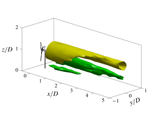
(a) Wall-normal variations of the time-averaged wind velocity  $U_{in}$, and the incoming turbulence intensity
 $I_{u}$. The symbols and the shaded rectangle indicate the hub location and the vertical range of the rotor, respectively. (b) Spatial evolution of the streamwise velocity contour in
 $yz$-planes, at
 $\unicode[STIX]{x1D6FD}=30^{\circ }$. Ticks on the
 $x$-axis correspond to the streamwise stations where stereo-PIV measurements are executed. (c) Isosurfaces of the wake velocity deficit
 $U_{w}$ and the streamwise vorticity
 $\unicode[STIX]{x1D714}_{x}$ at
 $\unicode[STIX]{x1D6FD}=30^{\circ }$. The outline of WIRE-01 turbine is indicated by black lines.

Figure 1(a) shows the wall-normal distributions of the mean streamwise velocity  $U_{in}$ and the streamwise turbulence intensity
 $I_{u}$, computed from 1000 samples of instantaneous velocity fields. Following the procedure described in Sciacchitano & Wieneke (Reference Sciacchitano and Wieneke2016), the relative measurement uncertainties of
 $U_{in}$ and
 $I_{u}$ caused by the finite sample size are estimated to be 0.2 % and 2 %, respectively. The boundary layer thickness determined from 99 % of the free-stream velocity is
 $\unicode[STIX]{x1D6FF}_{99}=0.3~\text{m}$, and the incoming turbulence intensity at hub level is 5.5 %, a relatively low value typically encountered by offshore wind farms (Türk & Emeis Reference Türk and Emeis2010). The Reynolds number based on the free-stream velocity and the boundary layer thickness reaches
 $Re_{\unicode[STIX]{x1D6FF}}=1.1\times 10^{5}$. Additionally, by fitting the measured velocity profile with a logarithmic law (Pope Reference Pope2000), the viscous velocity scale, length scale and aerodynamic roughness height are estimated to be
 $0.22~\text{m}~\text{s}^{-1}$, 0.068 mm and 0.7 mm, respectively.
In the case of turbine wake measurements, laser sheets are created in the cross-stream plane (i.e.  $yz$-plane) and thickened to 10 mm to reduce the particle pair losses caused by out-of-plane motion. Two cameras are viewing from the downstream of the wind turbine in an angle of approximately 40 degrees, and the two FOVs are overlapped by
 $3D\times 2.2D$. All the laser optics and the cameras are mounted on a high-precision motorized traversing system (ZABER X-LRT, range: 1500 mm), which allows automated wake measurements in the range of
 $0D<x\leqslant 10D$. For the purpose of subsequent model validation, five cases with different yaw angles (
 $\unicode[STIX]{x1D6FD}=-30^{\circ },-20^{\circ },-10^{\circ },0^{\circ },30^{\circ }$) are tested. In each case, 26 streamwise stations are selected to execute stereo PIV measurements, most of which are located within
 $0.2D\leqslant x\leqslant 5D$ where rapid wake deformation due to the vortices are expected to happen (Howland et al. Reference Howland, Bossuyt, Martínez-Tossas, Meyers and Meneveau2016). At each streamwise station, 1000 instantaneous velocity fields are sampled at a repetition rate of 10 Hz.
A representative spatial evolution of the streamwise velocity contour at  $\unicode[STIX]{x1D6FD}=30^{\circ }$ is shown in figure 1(b). Immediately downstream of the wind turbine, a large velocity deficit is observed in the shadow of tower and hub. Nevertheless, this localized high velocity deficit is quickly smeared out during downstream propagation, largely due to turbulent diffusion and wake rotation. Further downstream, the wake shifts preferentially towards the negative
 $y$-direction, departing from being elliptical in shape and curled strongly inside at above the hub level, which creates a top–down asymmetric kidney-shaped wake reported extensively in literature (Bastankhah & Porté-Agel Reference Bastankhah and Porté-Agel2016; Howland et al. Reference Howland, Bossuyt, Martínez-Tossas, Meyers and Meneveau2016; Vollmer et al. Reference Vollmer, Steinfeld, Heinemann and Kühn2016; Martínez-Tossas et al. Reference Martínez-Tossas, Annoni, Fleming and Churchfield2019). This three-dimensional wake deformation can be better visualized by the isosurface of the wake velocity deficit (
 $U_{w}$, computed as
 $U_{in}-U$) plotted in the left of figure 1(c) and is believed to be caused by vortex induction.
In the right plot of figure 1(c), two isosurfaces of the streamwise vorticity with opposite signs are shown. As evidenced, a CVP is created at  $x/D>3$. The upper leg of this CVP can be traced back to the negative streamwise vorticity shed from the rotor disk, while the lower leg seems to be rooted in the hub vortex. The positive vorticity shed at the bottom part of the rotor disk dissipates rapidly during downstream propagation. To further interpret how the streamwise vortices evolve into a CVP and the relationship between vortex evolution and wake deformation, theoretical analyses on the momentum equations of the wind turbine wake flow are needed (§ 3).
3 Momentum equations for wind turbine wake flow
Prior to the theoretical derivation, it is necessary to make a convention on the symbol usage:  $U$,
 $V$ and
 $W$ are the time-averaged velocity components in the
 $x$-,
 $y$- and
 $z$-directions, respectively; their lowercase counterparts, i.e.
 $u$,
 $v$ and
 $w$, represent the three instantaneous velocity components;
 $\langle \cdot \rangle$ is used to denote the ensemble averaging operation;
 $p$ and
 $\unicode[STIX]{x1D70C}$ are the air pressure and density, respectively;
 $\unicode[STIX]{x1D708}_{\unicode[STIX]{x1D706}}$ and
 $\unicode[STIX]{x1D708}_{T}$ represent the molecular viscosity and the eddy viscosity, respectively;
 $R$ and
 $a$ denote the rotor radius and the axial induction factor of wind turbine, respectively.
Without yaw, the axial induction factor is given by  $a=(1-\sqrt{1-C_{t}})/2$. With yaw, the detailed expression of the axial induction factor can be derived from the following two relations:
 $$\begin{eqnarray}\displaystyle C_{t}=\frac{T}{0.5\unicode[STIX]{x1D70C}U_{h}^{2}\unicode[STIX]{x03C0}R^{2}}, & & \displaystyle\end{eqnarray}$$
 $$\begin{eqnarray}\displaystyle T=\unicode[STIX]{x1D70C}U_{d}A_{ref}\unicode[STIX]{x0394}U, & & \displaystyle\end{eqnarray}$$
where the first equation is the canonical definition of the thrust coefficient, with  $T$ representing the streamwise force acting on the wind turbine, i.e. the thrust. The second equation is the integral form of the streamwise momentum equation, with
 $U_{d}$ and
 $\unicode[STIX]{x0394}U$ denoting respectively the averaged streamwise velocity at the rotor disk, and the streamwise velocity difference between inflow and outflow. Depending on the choice of the cross-section reference area (
 $A_{ref}$) and the definition of the axial induction factor in yaw, several expressions have been proposed in the literature (Burton, Sharpe & Jenkins Reference Burton, Sharpe and Jenkins2001; Bastankhah & Porté-Agel Reference Bastankhah and Porté-Agel2016). In the present study, the axial induction factor is defined as
 $a=1-U_{d}/U_{h}$, thus representing solely the induced velocity variation in the streamwise direction (instead of the disk-normal direction), leading to a simple expression of
 $\unicode[STIX]{x0394}U=2aU_{h}$. Moreover, if the stream tube containing the yawed rotor disk is selected as the control volume to apply the streamwise momentum equation, the cross-section area would be
 $A_{ref}=\unicode[STIX]{x03C0}R^{2}\cos (\unicode[STIX]{x1D6FD})$. Substituting these relations into equations (3.1)–(3.2), the axial induction factor of a yawed wind turbine can be obtained,
 $a=(1-\sqrt{1-C_{t}/\text{cos}(\unicode[STIX]{x1D6FD})})/2$.
In the present study, force measurements are not executed, and the data published in Bastankhah & Porté-Agel (Reference Bastankhah and Porté-Agel2016) are used to fit the thrust coefficient as a function of the yaw angle, i.e.  $C_{t}=0.82\cos (\unicode[STIX]{x1D6FD})^{1.6}$. Consequently, we have
 $$\begin{eqnarray}a=\left.\left(1-\sqrt{1-0.82\cos (\unicode[STIX]{x1D6FD})^{0.6}}\right)\right/2.\end{eqnarray}$$
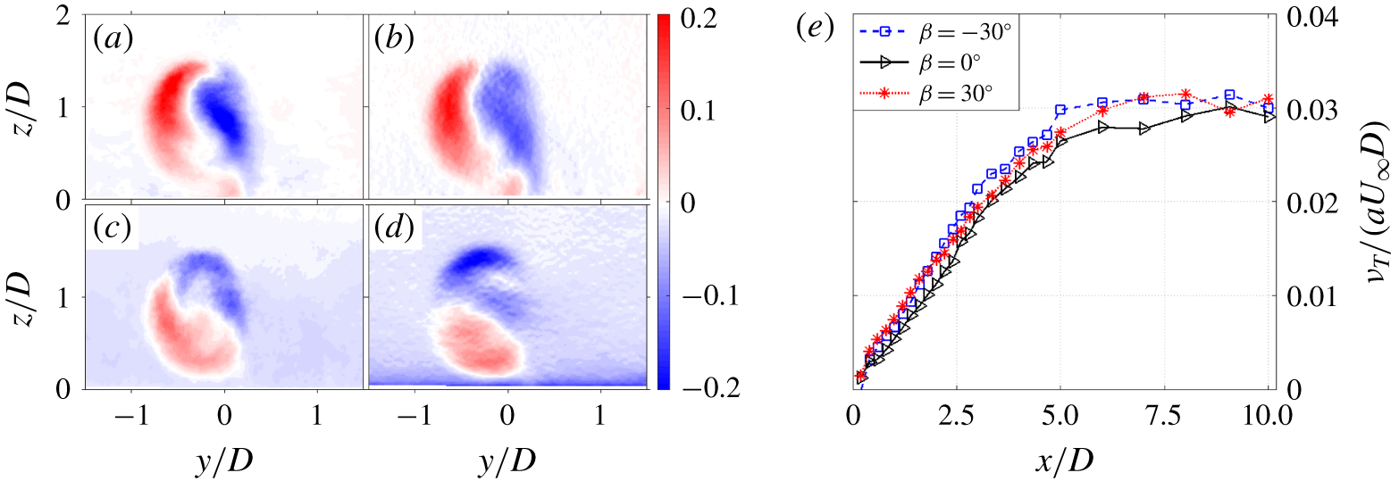
(a–d) Contours of  $\langle uv\rangle$,
 $-\unicode[STIX]{x1D708}_{T}\unicode[STIX]{x2202}U/\unicode[STIX]{x2202}y$,
 $\langle uw\rangle$ and
 $-\unicode[STIX]{x1D708}_{T}\unicode[STIX]{x2202}U/\unicode[STIX]{x2202}z$ at a yaw angle of
 $\unicode[STIX]{x1D6FD}=30^{\circ }$ and a streamwise location of
 $x/D=3$. (e) Streamwise variations of the normalized eddy viscosity for three representative yaw angles.

3.1 Simplification of the streamwise momentum equation
The complete form of the Reynolds-averaged momentum equation in  $x$-direction for incompressible wake flow is
 $$\begin{eqnarray}U\frac{\unicode[STIX]{x2202}U}{\unicode[STIX]{x2202}x}+V\frac{\unicode[STIX]{x2202}U}{\unicode[STIX]{x2202}y}+W\frac{\unicode[STIX]{x2202}U}{\unicode[STIX]{x2202}z}=\frac{1}{\unicode[STIX]{x1D70C}}\frac{\unicode[STIX]{x2202}p}{\unicode[STIX]{x2202}x}+\unicode[STIX]{x1D708}_{\unicode[STIX]{x1D706}}\unicode[STIX]{x1D6FB}^{2}U-\frac{\unicode[STIX]{x2202}\langle uu\rangle }{\unicode[STIX]{x2202}x}-\frac{\unicode[STIX]{x2202}\langle uv\rangle }{\unicode[STIX]{x2202}y}-\frac{\unicode[STIX]{x2202}\langle uw\rangle }{\unicode[STIX]{x2202}z}.\end{eqnarray}$$
This equation can be simplified based on the following considerations. Firstly, the diffusion term due to molecular viscosity, namely  $\unicode[STIX]{x1D708}_{\unicode[STIX]{x1D706}}\unicode[STIX]{x1D6FB}^{2}U$, can be readily ignored everywhere except for the near-wall viscous sublayer, since the Reynolds number for a utility-scale wind turbine is of the order of
 $10^{6}$–
 $10^{7}$. Secondly, the streamwise pressure gradient term
 $\unicode[STIX]{x2202}p/\unicode[STIX]{x2202}x$ becomes insignificant at
 $x/D\geqslant 2$ and thus can be omitted, considering our prime concern is the power yield prediction at an inter-turbine spacing of more than three rotor diameters. Finally, for simple shear flows like wakes, the gradient of Reynolds stresses in the streamwise direction is typically one order of magnitude less than that in the spanwise and wall-normal directions, resulting in a negligible contribution of
 $\unicode[STIX]{x2202}\langle uu\rangle /\unicode[STIX]{x2202}x$ to turbulent diffusion. After these simplifications, the streamwise momentum equation now reads
 $$\begin{eqnarray}U\frac{\unicode[STIX]{x2202}U}{\unicode[STIX]{x2202}x}+V\frac{\unicode[STIX]{x2202}U}{\unicode[STIX]{x2202}y}+W\frac{\unicode[STIX]{x2202}U}{\unicode[STIX]{x2202}z}\approx -\frac{\unicode[STIX]{x2202}\langle uv\rangle }{\unicode[STIX]{x2202}y}-\frac{\unicode[STIX]{x2202}\langle uw\rangle }{\unicode[STIX]{x2202}z}.\end{eqnarray}$$
To further eliminate the Reynolds stress terms, eddy viscosity assumptions are applied to equation (3.5), namely  $-\langle uv\rangle =\unicode[STIX]{x1D708}_{T}\unicode[STIX]{x2202}U/\unicode[STIX]{x2202}y$, and
 $-\langle uw\rangle =\unicode[STIX]{x1D708}_{T}\unicode[STIX]{x2202}U/\unicode[STIX]{x2202}z$ (Pope Reference Pope2000). Similar to other types of shear flows (e.g. plane wake, shear layer), the eddy viscosity
 $\unicode[STIX]{x1D708}_{T}$ is assumed to be uniform in the cross-stream plane, dependent only on the
 $x$-coordinate. The exact value of
 $\unicode[STIX]{x1D708}_{T}(x)$ can be computed by performing a linear regression between the Reynolds shear stress vector (
 $\langle uv\rangle$,
 $\langle uw\rangle$) and the velocity gradient vector (
 $\unicode[STIX]{x2202}U/\unicode[STIX]{x2202}y$,
 $\unicode[STIX]{x2202}U/\unicode[STIX]{x2202}z$) at each streamwise location. Figure 2(a–d) shows several representative spatial distributions of the Reynolds shear stresses obtained from experiments and eddy viscosity modelling at a streamwise location of
 $x/D=3$, in the case of
 $\unicode[STIX]{x1D6FD}=30^{\circ }$. As evidenced, for wind turbine wake flows, the eddy viscosity assumption can reasonably reproduce the spatial distributions of Reynolds shear stresses, and the domain-averaged covariance coefficient between experimental and modelled values is higher than 0.8.
Figure 2(e) plots the streamwise variations of the eddy viscosity in three different cases. The peak velocity difference across the wake,  $2aU_{\infty }$, and half of the initial wake width,
 $0.5D$, are selected as the reference velocity and length scales for normalization, resulting in a dimensionless eddy viscosity coefficient
 $\hat{\unicode[STIX]{x1D708}}_{T}=\unicode[STIX]{x1D708}_{T}/(aU_{\infty }D)$. This coefficient increases linearly at
 $x/D<5$ and remains unchanged afterwards, being independent of the yaw angle. The initial linear increase of
 $\unicode[STIX]{x1D708}_{T}$ can be interpreted from the perspective of the wake shear layer. Specifically, right behind the rotor disk, a circular shear layer emanates from the rotor edge and expands monotonically during its downstream propagation before reaching the wake centre at approximately
 $x=4D$ (not shown). This leads to an increasing characteristic length scale and consequently an increasing eddy viscosity. In the far wake, the increasing trend of eddy viscosity caused by wake width expansion is largely counteracted by the decreasing velocity difference across the wake, resulting in a plateau at
 $x/D>5$. Based on these observations, equation (3.6) is proposed to model eddy viscosity. Note that, under no circumstances are the constants in equation (3.6) universal. Further investigations are needed to incorporate the effects of turbulence intensity and thermal instability.
 $$\begin{eqnarray}\unicode[STIX]{x1D708}_{T}=\text{min}\{0.03,0.006x/D\}\times aU_{\infty }D.\end{eqnarray}$$
Additionally, the wind turbine in this study is submerged within a turbulent boundary layer. Taking the incoming wind profile  $U_{in}(z)$ as the reference velocity, the wake velocity deficit
 $U_{w}$ can be defined as
 $U_{w}(x,y,z)=U_{in}(z)-U(x,y,z)$. Substituting this relationship together with the eddy viscosity assumptions into equation (3.5), the following relation can be derived,
 $$\begin{eqnarray}(U_{in}-U_{w})\frac{\unicode[STIX]{x2202}U_{w}}{\unicode[STIX]{x2202}x}+V\frac{\unicode[STIX]{x2202}U_{w}}{\unicode[STIX]{x2202}y}+W\frac{\unicode[STIX]{x2202}U_{w}}{\unicode[STIX]{x2202}z}\approx W\frac{\unicode[STIX]{x2202}U_{in}}{\unicode[STIX]{x2202}z}+\unicode[STIX]{x1D708}_{T}\frac{\unicode[STIX]{x2202}^{2}U_{w}}{\unicode[STIX]{x2202}^{2}y}+\unicode[STIX]{x1D708}_{T}\frac{\unicode[STIX]{x2202}^{2}U_{w}}{\unicode[STIX]{x2202}^{2}z}.\end{eqnarray}$$
Strictly speaking, there should be another diffusion term on the right side of the above equation caused by the non-uniform boundary layer velocity profile, i.e.  $\unicode[STIX]{x1D708}_{T}\unicode[STIX]{x2202}^{2}U/\unicode[STIX]{x2202}^{2}z$. This term tends to flatten the incoming velocity profile even in the situation of no wake interference (i.e.
 $U_{w},V,W=0$) and thus has to be balanced by a streamwise pressure gradient to guarantee
 $U_{in}$ is independent of
 $x$, as in the case of channel flow. Since the pressure gradient term has already been omitted in the previous analysis,
 $\unicode[STIX]{x1D708}_{T}\unicode[STIX]{x2202}^{2}U/\unicode[STIX]{x2202}^{2}z$ is also discarded in equation (3.7). Otherwise, the original logarithmic velocity profile would be brought into a uniform velocity profile. Equation (3.7) is similar to the equation (4) derived in Martínez-Tossas et al. (Reference Martínez-Tossas, Annoni, Fleming and Churchfield2019) based on small disturbance assumptions. It is essentially a nonlinear transportation–diffusion equation of the wake velocity deficit, with an additional term
 $W\unicode[STIX]{x2202}U_{in}/\unicode[STIX]{x2202}z$ on the right side. Under the condition of uniform inflow, this additional term vanishes. In contrast, in a turbulent boundary layer,
 $W\unicode[STIX]{x2202}U_{in}/\unicode[STIX]{x2202}z$ can be either a production term of the wake deficit momentum (upwash,
 $W>0$), or a destruction term (downwash,
 $W<0$).
3.2 Simplification of the cross-stream momentum equations
Our prime concern is the three-dimensional wake evolution in yawed conditions. If, by some means, the cross-stream velocity fields are known everywhere a priori (e.g. cases of no wake rotation and zero yaw:  $V,W=0$), equation (3.7) can be solved numerically by implementing a downstream marching scheme in the
 $x$-direction. Following this roadmap, efforts will be made in the current section to decouple the cross-stream momentum equations from the streamwise one, so that an approximate solution of
 $V$ and
 $W$ can be obtained in the whole wake domain in advance.
The Reynolds-averaged momentum equations in the spanwise and wall-normal directions for wind turbine wake flow can be written as follows:
 $$\begin{eqnarray}\displaystyle & \displaystyle U\frac{\unicode[STIX]{x2202}V}{\unicode[STIX]{x2202}x}+V\frac{\unicode[STIX]{x2202}V}{\unicode[STIX]{x2202}y}+W\frac{\unicode[STIX]{x2202}V}{\unicode[STIX]{x2202}z}\approx -\frac{1}{\unicode[STIX]{x1D70C}}\frac{\unicode[STIX]{x2202}P}{\unicode[STIX]{x2202}y}-\frac{\unicode[STIX]{x2202}\langle vv\rangle }{\unicode[STIX]{x2202}y}-\frac{\unicode[STIX]{x2202}\langle vw\rangle }{\unicode[STIX]{x2202}z}, & \displaystyle\end{eqnarray}$$
 $$\begin{eqnarray}\displaystyle & \displaystyle U\frac{\unicode[STIX]{x2202}W}{\unicode[STIX]{x2202}x}+V\frac{\unicode[STIX]{x2202}W}{\unicode[STIX]{x2202}y}+W\frac{\unicode[STIX]{x2202}W}{\unicode[STIX]{x2202}z}\approx -\frac{1}{\unicode[STIX]{x1D70C}}\frac{\unicode[STIX]{x2202}P}{\unicode[STIX]{x2202}z}-\frac{\unicode[STIX]{x2202}\langle vw\rangle }{\unicode[STIX]{x2202}y}-\frac{\unicode[STIX]{x2202}\langle ww\rangle }{\unicode[STIX]{x2202}z}, & \displaystyle\end{eqnarray}$$
where the streamwise gradients of the Reynolds shear stresses (i.e.  $\unicode[STIX]{x2202}\langle uv\rangle /\unicode[STIX]{x2202}x$ and
 $\unicode[STIX]{x2202}\langle uw\rangle /\unicode[STIX]{x2202}x$) are neglected.
Assuming that the incoming flow is uniform and the wake velocity deficit is small, negligible errors will be incurred if  $U(x,y,z)$ in the first term of equations (3.8)–(3.9) is replaced by the averaged wake convection velocity in the cross-stream plane
 $U_{m}(x)$. Further, if a dummy convection time variable
 $t$ (not the physical time) is defined differentially from
 $\text{d}t=\text{d}x/U_{m}$, the original cross-stream momentum equations can be reformulated into a stand-alone two-dimensional momentum equation set, by virtue of the chain rule, as follows:
 $$\begin{eqnarray}\displaystyle & \displaystyle \frac{\unicode[STIX]{x2202}V}{\unicode[STIX]{x2202}t}+V\frac{\unicode[STIX]{x2202}V}{\unicode[STIX]{x2202}y}+W\frac{\unicode[STIX]{x2202}V}{\unicode[STIX]{x2202}z}\approx -\frac{1}{\unicode[STIX]{x1D70C}}\frac{\unicode[STIX]{x2202}P}{\unicode[STIX]{x2202}y}-\frac{\unicode[STIX]{x2202}\langle vv\rangle }{\unicode[STIX]{x2202}y}-\frac{\unicode[STIX]{x2202}\langle vw\rangle }{\unicode[STIX]{x2202}z}, & \displaystyle\end{eqnarray}$$
 $$\begin{eqnarray}\displaystyle & \displaystyle \frac{\unicode[STIX]{x2202}W}{\unicode[STIX]{x2202}t}+V\frac{\unicode[STIX]{x2202}W}{\unicode[STIX]{x2202}y}+W\frac{\unicode[STIX]{x2202}W}{\unicode[STIX]{x2202}z}\approx -\frac{1}{\unicode[STIX]{x1D70C}}\frac{\unicode[STIX]{x2202}P}{\unicode[STIX]{x2202}z}-\frac{\unicode[STIX]{x2202}\langle vw\rangle }{\unicode[STIX]{x2202}y}-\frac{\unicode[STIX]{x2202}\langle ww\rangle }{\unicode[STIX]{x2202}z}. & \displaystyle\end{eqnarray}$$
In this equation set, the streamwise coordinate (i.e.  $x$) no longer exists, and the dummy convection time variable becomes one of the independent variables, indicating that if one follows the mean convection of the wake, the streamwise evolution of the cross-stream velocity field can be viewed approximately as a temporal evolution. With the initial condition specified, equations (3.10)–(3.11) can be solved numerically, e.g. using the semi-implicit method for pressure linked equations (Anderson et al. Reference Anderson, Degrez, Dick and Grundmann2013). Nevertheless, this numerical approach is computationally expensive, and an alternative vortex method is sought in the next section to work out the cross-stream velocities required by equation (3.7). The configuration of the vortex system is detailed in § 4.1. The time evolution of the vortices due to mutual induction is simulated in § 4.2. In §§ 4.3–4.4, the wake deformation process and the integral parameters relevant to yawed wind turbines (i.e. wake deflection, available power) are analysed, respectively.
4 Point vortex transportation model
4.1 Initialization of the cross-stream velocity field with point vortices
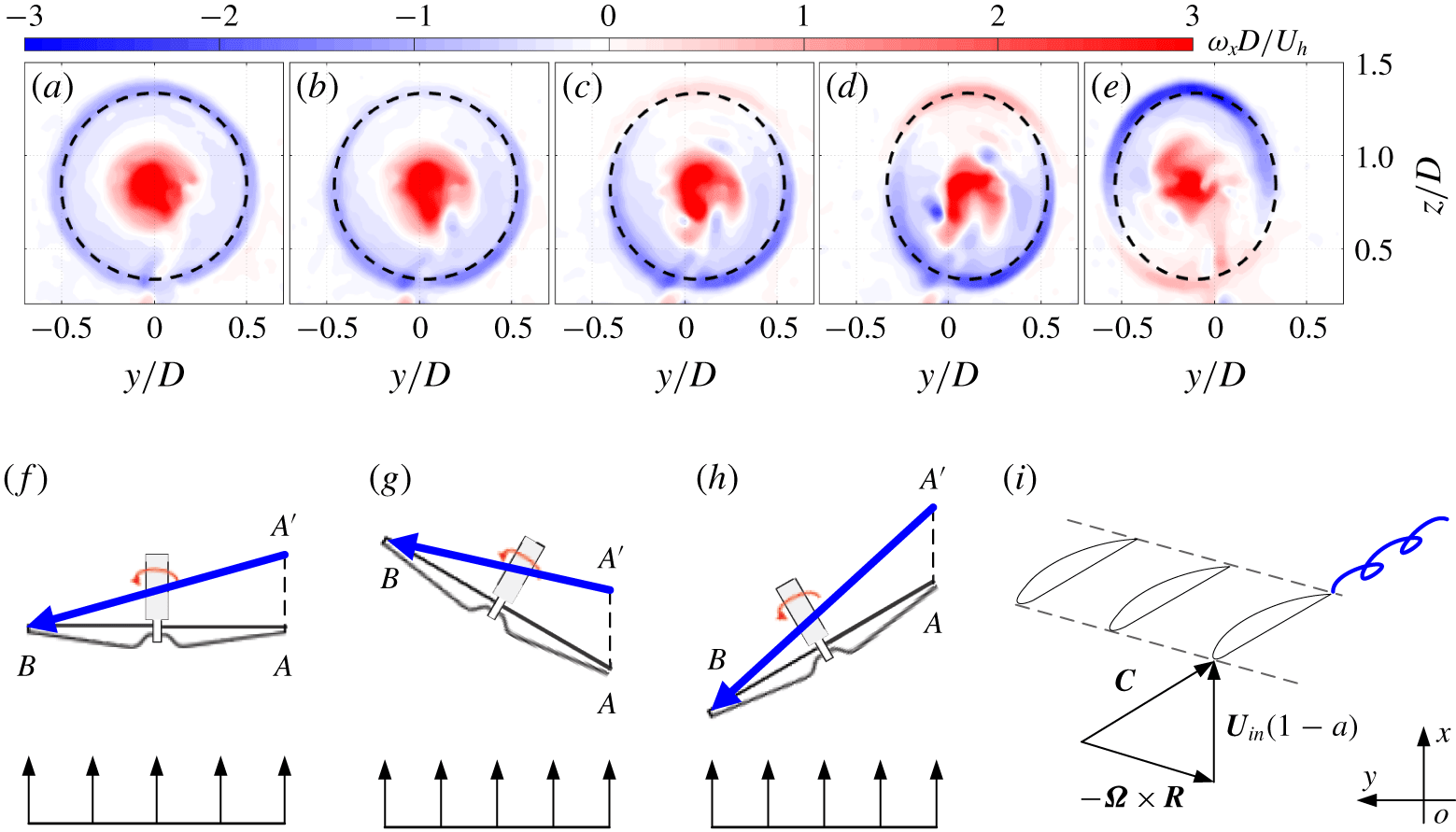
(a–e) Streamwise vorticity contours at  $x/D=0.4$ for five different yaw angles. From left to right:
 $\unicode[STIX]{x1D6FD}=0^{\circ },-10^{\circ },-20^{\circ },-30^{\circ },30^{\circ }$. Dashed lines indicate the streamwise projection of the rotor disk. (f–h) Sketches of the tip vortex trajectories at
 $\unicode[STIX]{x1D6FD}=0^{\circ }$ (f),
 $\unicode[STIX]{x1D6FD}=-30^{\circ }$ (g) and
 $30^{\circ }$ (h), when the rotor blades are sweeping from point
 $A$ to point
 $B$. The orientation of each vortex is indicated by a thick blue arrow. (i) Sketch of the velocity triangle at the blade tip under yawed conditions.

For all of the five yaw angles tested, the spatial distribution of the streamwise vorticity (denoted as  $\unicode[STIX]{x1D714}_{x}$) just behind the rotor disk at
 $x/D=0.4$ is shown in figure 3(a–e). The time-averaged hub velocity
 $U_{h}$ and the rotor diameter
 $D$ are used as the reference velocity and length scales to non-dimensionalize
 $\unicode[STIX]{x1D714}_{x}$. Without yaw, positive vorticity is concentrated in the rotor centre corresponding to the hub vortex, and negative vorticity is distributed uniformly along the rotor edge, pertaining to the streamwise component of the tip vortices shed at the rotor disk periphery. Such a vorticity distribution is similar to that created in Taylor–Couette flow when the outer cylinder is non-rotating (Davey Reference Davey1962). Consequently, wake rotation is effectively confined inside the negative vorticity ring. When the wind turbine is yawed negatively (figure 3b–d), the negative vorticity shed from the bottom half of the rotor disk is enhanced noticeably, whereas that emanating from the upper half is first reduced (
 $\unicode[STIX]{x1D6FD}=-10^{\circ }$) and then transformed into positive vorticity at
 $\unicode[STIX]{x1D6FD}\leqslant -20^{\circ }$. In the case of positive yaw (figure 3e), the negative vorticity switches its sign in the bottom half of the rotor disk and agglomerates in the top half.
By integrating the streamwise vorticity across the entire measurement domain, it is found out that the net circulation induced by the hub vortex and the tip vortices amounts approximately to zero, regardless of the streamwise location and the yaw angle. This finding should not be surprising and can be interpreted from the theory of vortex dynamics. According to Saffman (Reference Saffman1992), the vorticity in the incompressible flow can only be created either by non-conservative body forces within a control volume or by near-wall pressure gradients working against the viscous forces on a solid boundary. In the current situation, non-conservative body forces such as the electromagnetic force are absent. If the control volume is selected large enough to contain the rotor disk yet away from the wall, the net vorticity flux at the outflow plane should be balanced out by that at the inflow plane. As the mean streamwise vorticity carried by the inflow turbulent boundary layer is zero, it is largely expected that at each of the downstream planes the net circulation should remain zero. In Bastankhah & Porté-Agel (Reference Bastankhah and Porté-Agel2016) and Martínez-Tossas et al. (Reference Martínez-Tossas, Annoni, Fleming and Churchfield2019), the cross-stream velocity field is simulated by a combination of a counter-rotating vortex pair and a hub vortex, which is unphysical due to the violation of the zero-net circulation rule.
To further reveal the physics of vorticity sign switch at large yaw angles, the trajectory of a tip vortex created by blades sweeping from right to left is indicated in figure 3(f–h) (top view, wind blows from the bottom). As depicted, a tip vortex segment is initially shed from the rotor blade at point  $A$ and subsequently starts convecting downstream at a mean speed of
 $(1-a)U_{\infty }$. Half a cycle later, the head of this vortex segment is propagated to point
 $A^{\prime }$, while its tail is still attached at the blade tip swept to point
 $B$. Without yaw (figure 3f), point
 $A^{\prime }$ is always located downstream of point
 $B$, resulting in an upstream-oriented tip vortex segment (
 $\overrightarrow{A^{\prime }B}$) which can be projected into the
 $x$-direction as a negative streamwise vortex. However, if the rotor disk is yawed negatively so much that point
 $A^{\prime }$ is lagged behind point
 $B$ (figure 3g), the tip vortex segment
 $\overrightarrow{A^{\prime }B}$ will point slightly downstream and give rise to positive streamwise vorticity in the top half of the rotor, which is consistent with figure 3(d). On the contrary, positive yaw angles will result in a tip vortex segment inclined severely upstream (figure 3h), which creates a high level of negative streamwise vorticity in the top half of the rotor. The transition yaw angle (
 $\unicode[STIX]{x1D6FD}_{T}$) beyond which the streamwise vorticity shed from the rotor disk starts to change signs locally, can be derived from the relation of
 $|AA^{\prime }|=|AB|\text{cos}(\unicode[STIX]{x1D6FD})$, as follows:
 $$\begin{eqnarray}\unicode[STIX]{x1D6FD}_{T}=\pm \text{asin}\left(\frac{1-a}{\unicode[STIX]{x1D706}_{t}}\right),\end{eqnarray}$$
where  $\unicode[STIX]{x1D706}_{t}$ denotes the tip speed ratio determined by
 $|\unicode[STIX]{x1D6FA}|R/U_{h}$. In this study, the transition yaw angle is computed to be
 $\pm 11.5^{\circ }$, in agreement with figure 3(b–c).
As a generalization of the above findings, the strength of the streamwise vorticity at a certain circumferential location depends on both the local trajectory and the total strength of the blade tip vortices. Figure 3(i) sketches the velocity triangle at the blade tip in yawed conditions. The compound velocity seen by the airfoil defines the local tip vortex trajectory and is given by  $\boldsymbol{C}=\boldsymbol{U}_{in}(1-a)-\unicode[STIX]{x1D734}\times \boldsymbol{R}$. Note that the tangential velocity vector
 $\unicode[STIX]{x1D734}\times \boldsymbol{R}$ is dependent on both the yaw angle and the blade phase angle (denoted as
 $\unicode[STIX]{x1D719}$);
 $\unicode[STIX]{x1D719}$ is referenced as zero when the blade or its projection in the cross-stream plane is oriented in the positive
 $y$-direction, thus increasing in the counter-clockwise direction when viewing from downstream. Bearing this in mind, it is just a matter of coordinate transformation to derive the following expression of the compound velocity:
 $$\begin{eqnarray}\boldsymbol{C}=\left[\begin{array}{@{}c@{}}U_{in}(1-a)-\unicode[STIX]{x1D6FA}R\sin (\unicode[STIX]{x1D719})\sin (\unicode[STIX]{x1D6FD})\\ -\unicode[STIX]{x1D6FA}R\sin (\unicode[STIX]{x1D719})\cos (\unicode[STIX]{x1D6FD})\\ \unicode[STIX]{x1D6FA}R\cos (\unicode[STIX]{x1D719})\end{array}\right].\end{eqnarray}$$
The total circulation of the streamwise vorticity shed from the blade tips ( $\unicode[STIX]{x1D6E4}$) is available from the vortex cylinder theory of wind turbine wakes (Burton et al. Reference Burton, Sharpe and Jenkins2001; Branlard & Gaunaa Reference Branlard and Gaunaa2015), as a function of the wind velocity, angular velocity and thrust coefficient
 $$\begin{eqnarray}\unicode[STIX]{x1D6E4}_{0}=k\unicode[STIX]{x03C0}U_{h}^{2}C_{t}/\unicode[STIX]{x1D6FA}(1+a^{\prime }),\end{eqnarray}$$
where  $a^{\prime }$ is the tangential induction factor at the blade tip and can be ignored in the case of large tip speed ratio;
 $k$ is a factor added artificially to account for the overprediction of total circulation caused by the assumptions made during the derivation of equation (4.3), as will be dealt in a later stage. For now, we will continue the analysis without correction, i.e.
 $k=1$. A simple case of uniform inflow is first considered, where the strength of a tip vortex is unrelated to its circumferential location. If the whole rotor disk is divided evenly into
 $N$ arc segments, the circulation pertaining to the
 $i$th segment (denoted as
 $\unicode[STIX]{x1D6E4}_{i}$) would be proportional to the streamwise projection of the normalized local compound velocity vector
 $\boldsymbol{C}_{i}/|\boldsymbol{C}_{i}|$. As such, equation (4.4) can be used to distribute the total circulation among all the arc segments, where
 $\boldsymbol{e}_{x}$ denotes the unit vector along the
 $x$-direction,
 $$\begin{eqnarray}\unicode[STIX]{x1D6E4}_{i}=\unicode[STIX]{x1D6E4}_{0}\boldsymbol{\cdot }\frac{\boldsymbol{e}_{x}\boldsymbol{\cdot }\boldsymbol{C}_{i}/|\boldsymbol{C}_{i}|}{\displaystyle \mathop{\sum }_{i=1}^{i=N}\boldsymbol{e}_{x}\boldsymbol{\cdot }\boldsymbol{C}_{i}/|\boldsymbol{C}_{i}|}.\end{eqnarray}$$
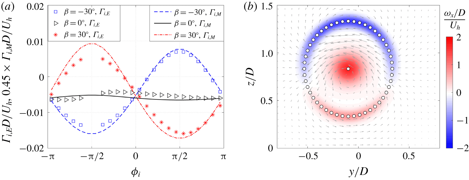
(a) Comparison of the circulation obtained from experiments ( $\unicode[STIX]{x1D6E4}_{i,E}$) and equation (4.4) (
 $\unicode[STIX]{x1D6E4}_{i,M}$) at three different yaw angles. Note that in the vertical axis
 $\unicode[STIX]{x1D6E4}_{i,M}$ is multiplied by a factor of 0.45. (b) The initial cross-stream velocity and vorticity fields reconstructed from the proposed point vortex system, at
 $\unicode[STIX]{x1D6FD}=30^{\circ }$. The spatial locations of the point vortices are indicated by circles. Note that the mirror vortices in the negative
 $z$ side are not shown.

To validate the accuracy of equation (4.4), experimental data of  $\unicode[STIX]{x1D6E4}_{i}$ at
 $\unicode[STIX]{x1D6FD}=-30^{\circ },0^{\circ },30^{\circ }$ are extracted from figure 3. Specifically, the ring area of
 $0.4D\leqslant \sqrt{y^{2}+z^{2}}\leqslant 0.6D$ is divided evenly into 24 arc segments, and the streamwise vorticity inside each arc segment is integrated to obtain the local circulation. Figure 4(a) compares the circumferential variations of the circulation obtained from experiments and model (differentiated by the subscriptions,
 $\unicode[STIX]{x1D6E4}_{i,E}$ and
 $\unicode[STIX]{x1D6E4}_{i,M}$). The rotor diameter
 $D$ and the mean hub velocity
 $U_{h}$ are used for non-dimensionalization. Qualitatively, the trend given by the model agrees well with that from the experiments. Nevertheless, quantitatively, equation (4.4) largely overestimates the strength of the streamwise vortices, and the experimental circulation values are only 45 % of the modelled values. This over-prediction can be ascribed to the assumptions of zero drag and constant circulation distribution along the blade span during the derivation of equation (4.3) (Burton et al. Reference Burton, Sharpe and Jenkins2001; Branlard & Gaunaa Reference Branlard and Gaunaa2015).
Specifically, when drag is non-negligible, only part of the thrust can be linked to the creation of circulation, and the thrust coefficient  $C_{t}$ in equation (4.3) has to be reduced to yield a correct prediction of
 $\unicode[STIX]{x1D6E4}_{0}$. For the case of non-uniform circulation distribution along the blade span, part of the vorticity is shed in the blade middle instead of the blade tip, leading to the total circulation of the tip vortices less than
 $\unicode[STIX]{x1D6E4}_{0}$ (Anderson Reference Anderson2010). These factors can be taken into account by the blade element momentum theory, which, however, requires detailed information of the blade geometry. To avoid further complicating the calculation of total circulation, the factor
 $k$ in equation (4.3) is set as 0.45 to counteract the model overestimation.
With the efforts made above, it becomes feasible to reconstruct the initial cross-stream velocity field with a cloud of point vortices. The proposed vortex system consists of a hub vortex located in the centre of the rotor disk whose circulation is  $-\unicode[STIX]{x1D6E4}_{0}$, and
 $N$ point vortices distributed evenly along the rotor disk edge with circulation
 $\unicode[STIX]{x1D6E4}_{i}$ given by equation (4.4). To further mimic the ground effect, these
 $N+1$ point vortices are mirrored against
 $z=0$ to ensure the no-penetration condition. In this vortex configuration, the zero-net total circulation criterion is automatically satisfied. For each of the point vortices centred at
 $(y_{c}^{i},z_{c}^{i})$ (
 $i=1,2,\ldots ,2N+1$), its induced velocity field
 $(V_{i},W_{i})$ is given by the Lamb–Oseen viscous vortex model (Wu, Ma & Zhou Reference Wu, Ma and Zhou2007) as follows:
 $$\begin{eqnarray}\displaystyle & \displaystyle V_{i}(x,y,t)=\frac{-\unicode[STIX]{x1D6E4}_{i}(z-z_{c}^{i})}{2\unicode[STIX]{x03C0}[(y-y_{c}^{i})^{2}+(z-z_{c}^{i})^{2}]}\left[1-\text{exp}\left(-\frac{(y-y_{c}^{i})^{2}+(z-z_{c}^{i})^{2}}{4\unicode[STIX]{x1D708}_{E}t+R_{i}^{2}}\right)\right], & \displaystyle\end{eqnarray}$$
 $$\begin{eqnarray}\displaystyle & \displaystyle W_{i}(x,y,t)=\frac{-\unicode[STIX]{x1D6E4}_{i}(y-y_{c}^{i})}{2\unicode[STIX]{x03C0}[(y-y_{c}^{i})^{2}+(z-z_{c}^{i})^{2}]}\left[1-\text{exp}\left(-\frac{(y-y_{c}^{i})^{2}+(z-z_{c}^{i})^{2}}{4\unicode[STIX]{x1D708}_{E}t+R_{i}^{2}}\right)\right], & \displaystyle\end{eqnarray}$$
where  $R_{i}$ is the initial radius of the point vortex, set as
 $0.15D$ for the hub vortex and
 $0.05D$ for the rest according to experimental observations;
 $\unicode[STIX]{x1D708}_{E}$ denotes the eddy viscosity in the cross-stream plane, defined from the Reynolds stresses and mean strain rates (Pope Reference Pope2000). In this study, the following expression is used,
 $\unicode[STIX]{x1D708}_{E}=0.03\unicode[STIX]{x1D6E4}_{0}/2\unicode[STIX]{x03C0}=0.005\unicode[STIX]{x1D6E4}_{0}$. Namely, the maximum vortex-induced velocity
 $\unicode[STIX]{x1D6E4}_{0}/2\unicode[STIX]{x03C0}R_{i}$ and the corresponding vortex radius
 $R_{i}$ are selected as the reference velocity and length scales for eddy viscosity estimation, and a factor of 0.03 is multiplied for scaling, analogous to equation (3.6).
Figure 4(b) shows the initial cross-stream velocity field ( $t=0$) reconstructed from a cloud of 101 point vortices at yaw angle of
 $\unicode[STIX]{x1D6FD}=30^{\circ }$. As evidenced from the comparison with figure 3, the non-uniform vorticity distribution in the periphery of the rotor disk is reproduced accurately. At this initial state, the vortex cloud induces a strong negative transverse velocity in the upper half of the rotor disk yet a rather weak transverse velocity in the bottom half. It can be imagined that, driven by such a cross-stream velocity pattern, the initial elliptical wake profile will lean slightly to the negative
 $y$-axis and lose its top–down symmetry.
4.2 Evolution of cross-stream velocity field under mutual induction
During the evolution of streamwise vortices, two effects are prominent. One is the diffusion of vorticity due to the eddy viscosity which has already been incorporated in the Lamb–Oseen vortex model, and the other is the transportation of vorticity because of mutual induction. Assuming the induced velocity of point vortices can be superimposed linearly, the time evolution of the  $j$th vortex centre (
 $y_{c}^{j},z_{c}^{j}$) can be written in the following differential form:
 $$\begin{eqnarray}\displaystyle & \displaystyle \frac{\text{d}y_{c}^{j}}{\text{d}t}=\mathop{\sum }_{i=1}^{i=N+1}V_{i}(x_{c}^{j},y_{c}^{j},t)(1-\unicode[STIX]{x1D6FF}_{i,j}), & \displaystyle\end{eqnarray}$$
 $$\begin{eqnarray}\displaystyle & \displaystyle \frac{\text{d}z_{c}^{j}}{\text{d}t}=\mathop{\sum }_{i=1}^{i=N+1}W_{i}(x_{c}^{j},y_{c}^{j},t)(1-\unicode[STIX]{x1D6FF}_{i,j}), & \displaystyle\end{eqnarray}$$
where  $\unicode[STIX]{x1D6FF}_{i,j}$ is the Dirichlet function, equalling 1 if
 $i=j$ and 0 otherwise.
These two equations, together with equations (4.2)–(4.6) in § 4.1, constitute a closed equation set which can be used to simulate the evolution of cross-stream velocity field under any operation condition, as long as the geometrical and operational parameters of the wind turbine ( $R$,
 $U_{in}$,
 $\unicode[STIX]{x1D6FA}$,
 $C_{t}$) are available. In this study, an explicit time-marching scheme is adopted to solve this ordinary equation set, and the time step is selected in such a way that the maximum convection distance of the vortex centre is less than one fifth of the minimum distance between any two point vortices. After each time update, if the distance between two neighbouring vortices becomes less than the initial vortex radius, vortex merging is invoked and these two neighbouring point vortices are combined into one. For a typical setting of
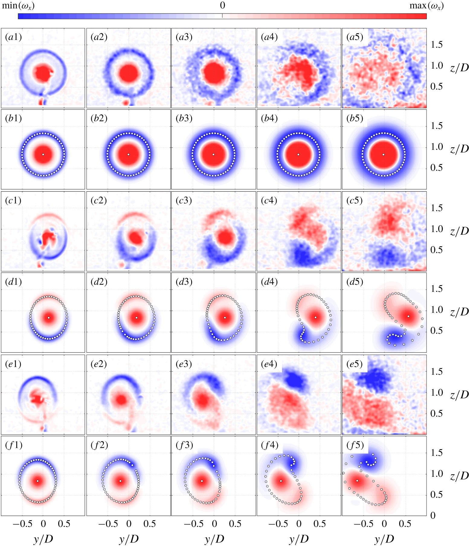
 $N=50$, only 0.1 second is needed to compute the complete evolution of the proposed point vortex system. In the appendix, some guidance on how to select the model parameters is provided. Figure 5 shows the streamwise vorticity contours obtained from both the point vortex system and the experiments, at
 $\unicode[STIX]{x1D6FD}=0^{\circ },-30^{\circ }$ and
 $30^{\circ }$. Note that, to facilitate comparison, the dummy convection time
 $t$ in model simulation is converted to the convection distance
 $x$ using
 $t=\int _{0}^{x}U_{m}(x)^{-1}\,\text{d}x$, as has been mentioned earlier in § 3.2. For the cross-stream vorticity evolution at other yaw angles, please refer to supplementary movies 1–5 available online at https://doi.org/10.1017/jfm.2020.123.
Comparison of the streamwise vorticity evolution measured in experiments (odd rows) and simulated by the point vortex model (even rows) at three yaw angles: (a1–b5)  $\unicode[STIX]{x1D6FD}=0^{\circ }$; (c1–d5)
 $\unicode[STIX]{x1D6FD}=-30^{\circ }$; (e1–f5)
 $\unicode[STIX]{x1D6FD}=30^{\circ }$. Note that these contours are plotted in their own range of the streamwise vorticity. For each row, from left to right, the corresponding streamwise coordinates/convection distances are
 $x/D=0.4$, 1, 2, 4 and 8, respectively. The spatial locations of the point vortices in the model are indicated by circles.

Without yaw, the point vortices residing initially near the rotor disk edge orbit around the hub vortex under mutual induction and maintain a stable circular pattern (see row (b) of figure 5). Experimental observations are consistent with the model predictions, illustrating a process governed by vorticity diffusion. Additionally, although no wake deflection is expected in this case, the streamwise vorticity in figure 5(a3,a4) exhibits an asymmetric distribution with respect to the  $z$-axis, which is ascribed to the vortex stretching/compression in three-dimensional space. Specifically, streamwise vortices on the right side are transported upwards by the hub vortex, experiencing a positive convective acceleration in the
 $x$-direction, i.e. vortex stretching. This vortex stretching leads to an increase of the vorticity and a shrinkage of the vortex diameter (Wu et al. Reference Wu, Ma and Zhou2007). In contrast, the streamwise vortices on the left side are compressed due to the negative convective acceleration and have to expand in diameter and decrease in vorticity. Since the point vortex model proposed in this paper is two-dimensional, this asymmetric vorticity distribution is not present in figure 5(b3,b4).
In the case of  $\unicode[STIX]{x1D6FD}=-30^{\circ }$, the vortices located in the top half of the wake share the same sign with the hub vortex (see rows (c,d) of figure 5). As a general rule in vortex dynamics, vortices sharing the same sign tend to orbit each other and organize themselves into a roughly circular shape (Wu et al. Reference Wu, Ma and Zhou2007; Saffman Reference Saffman1992). Considering this rule in the current situation, the vortices in the top half of the wake gradually get closer to each other during the initial evolution and subsequently merge with the hub vortex, creating a patch of positive vorticity at
 $x/D\leqslant 4$. Meanwhile, the negative vortices distributed in the bottom half of the wake are transported towards the bottom left corner by the hub vortex and curved into a negative vorticity patch under self-induction. These two patches with opposite signs of streamwise vorticity induce a positive transverse velocity in between and essentially constitute the CVP observed widely in studies of yawed wind turbines. Contrary to the interpretations in previous studies (Bastankhah & Porté-Agel Reference Bastankhah and Porté-Agel2016; Martínez-Tossas et al. Reference Martínez-Tossas, Annoni, Fleming and Churchfield2019), the hub vortex is not a third vortex independent from the CVP. Rather, it merges with part of the streamwise vorticity shed from the blade tips and forms one leg of the CVP.
The situation of  $\unicode[STIX]{x1D6FD}=30$ can be analysed in a similar fashion. Specifically, the positive vorticity distributed in the bottom half of the rotor disk agglomerates towards the bottom-right corner and merges with the hub vortex to form a patch of positive vorticity below the hub. In the meantime, the negative vorticity streak initially in a half-circle shape curls into a concentrated negative vorticity patch at the top-right corner of the rotor disk. Under mutual induction, these two patches of opposite vorticity will shift gradually to the negative
 $y$-direction afterwards. Actually, the top–down asymmetric kidney-shaped wake profile this study aims to reproduce is already manifested by the envelope of point vortices in figure 5(d5,f5). This is largely expected. Since the two-dimensional vorticity transportation equation in itself is a scalar transportation equation (Saffman Reference Saffman1992), the evolution of an initial elliptical vortex envelope should somehow resemble the actual wake deformation.
As evidenced from the above observations, the CVP formed behind a yawed wind turbine is fundamentally different from that created behind a drag disk. For a yawed drag disk, the hub vortex is absent, and both of the two legs of the CVP originate from the streamwise vorticity shed from the disk edge (Howland et al. Reference Howland, Bossuyt, Martínez-Tossas, Meyers and Meneveau2016; Shapiro et al. Reference Shapiro, Gayme and Meneveau2018), resulting in a top–down symmetric velocity field under uniform inflow conditions. In contrast, for the case of yawed wind turbines, since one leg of the CVP is rooted in the hub vortex, the induced transverse velocity is top–down asymmetric, and thus the wake of yawed wind turbines will always be top–down asymmetric even under uniform inflow conditions.
Additionally, the role of the hub vortex in wind turbine wake dynamics is not limited to wake deformation. The LES results from Kang, Yang & Sotiropoulos (Reference Kang, Yang and Sotiropoulos2014) and Foti et al. (Reference Foti, Yang, Campagnolo, Maniaci and Sotiropoulos2018) indicate that for non-yawed wind turbines, the unstable hub vortex can energize the wake meandering process and increase the turbulence level in the far-wake region. In the present point vortex model, the wake meandering phenomenon and the spiral instability of the hub vortex are not accounted for. Thus, it is not surprising to notice from the last column of figure 5 that even at a streamwise distance of  $x/D=8$, the model-predicted hub vortex is still well defined, dominating the spatial evolution of the positive vorticity patch. As a comparison, experimental results indicate that the concentrated hub vortex starts to break down into small-scale vortices at
 $x/D=4$ and subsequently merges with the adjacent part of positive vorticity. Since small-scale vortices dissipate faster than the large-scale vortex, the total circulation of the vortex system decreases noticeably in the far wake, as evidenced by figure 5(a5). In the present vortex model, the strength of the point vortices is assumed to be invariant, which will inevitably lead to an over-prediction of the transverse velocity and the resultant wake deflection at
 $x/D\leqslant 8$, as will be shown in § 4.4.
Evolution of the wake velocity deficit contours obtained from experiments (a–c) and the PVT model (d–f) at  $\unicode[STIX]{x1D6FD}=30^{\circ }$. In each row, from left to right, the corresponding streamwise coordinates are
 $x/D=3$, 6 and 10, respectively. In each panel, the in-plane velocity vector (
 $\boldsymbol{V}$,
 $\boldsymbol{W}$) is indicated by arrows, and the wake profile is indicated by the contour line of
 $U_{w}/U_{h}=0.1$.

4.3 Deformation of wake velocity deficit contour due to vortex transportation
With the cross-stream velocity fields computed in § 4.2 at hand, equation (3.7) can be solved numerically in the full wake domain. Since equation (3.7) exhibits mixed behaviours of both parabolic and hyperbolic equations, MacCormack method is deployed to march the solution in the  $x$-direction, and all the spatial derivatives are discretized using second-order central difference schemes (Anderson et al. Reference Anderson, Degrez, Dick and Grundmann2013). The spatial step
 $\unicode[STIX]{x0394}x$ is determined dynamically by the stability criteria of both elliptical and hyperbolic equations as follows:
 $$\begin{eqnarray}\unicode[STIX]{x0394}x=\unicode[STIX]{x0394}y\min \left\{\frac{\unicode[STIX]{x0394}yU_{m}}{2\unicode[STIX]{x1D708}_{T}},\frac{U_{m}}{V_{max}}\right\},\end{eqnarray}$$
where  $V_{max}$ denotes the maximum transverse velocity, and
 $\unicode[STIX]{x0394}y$ is the grid spacing in cross-stream planes. To determine the mean wake convection velocity (
 $U_{m}(x)$), a proper definition of the cross-stream wake boundary is needed. In the present study, this boundary is chosen as the contour line of
 $0.1\max (U_{w})$, i.e. 10 % of the maximum wake velocity deficit. The authors have also tested other threshold values (5 % and 20 % of
 $\max (U_{w})$), and the impact on the wake deflection and downstream available power is negligible. For a typical setting of
 $\unicode[STIX]{x0394}y=D/30$, it is the first term in equation (4.9) that limits the selection of
 $\unicode[STIX]{x0394}x$.
To launch the simulation, the initial condition of equation (3.7) is specified as a top-hat distribution of the wake velocity deficit
 $$\begin{eqnarray}U_{w}|_{x=0}=\left\{\begin{array}{@{}ll@{}}2aU_{h}, & \sqrt{(y+l_{n}\sin (\unicode[STIX]{x1D6FD}))^{2}/\cos ^{2}(\unicode[STIX]{x1D6FD})+(z-z_{h})^{2}}\leqslant R,\\[2.0pt] 0, & \text{otherwise},\end{array}\right.\end{eqnarray}$$
where  $l_{n}$ is the spacing between the tower and the rotor (0.03 m for WIRE01), accounting for the physical shift of the rotor disk centre caused by yaw. The effect of the tower-induced drag is included by adding an extra wake velocity deficit in the tower shadow region, analogous to the body force parametrization in Wu & Porté-Agel (Reference Wu and Porté-Agel2011). Depending on the size of the computational domain (e.g.
 $-2D\leqslant y\leqslant 2D,0\leqslant z\leqslant 3D$), approximately 2 seconds are needed to simulate the wake evolution between
 $x=0$ and
 $x=10D$, comparable to the computational cost of the curled wake model proposed by Martínez-Tossas et al. (Reference Martínez-Tossas, Annoni, Fleming and Churchfield2019).
Figure 6 compares the wake velocity deficit profiles obtained from the proposed model and the experiments at  $\unicode[STIX]{x1D6FD}=30^{\circ }$. The model prediction results agree well with the experimental data, both demonstrating that the evolution of wake velocity deficit is governed by turbulent diffusion and cross-stream vortex transportation. Turbulent diffusion controls how fast the wake boundary expands and the peak wake velocity deficit decreases, while cross-stream vortex transportation redistributes the wake velocity deficit and determines the overall wake shape. For all the plots shown in figure 6, the CVP is located in the upper half of rotor disk, and the induced negative transverse velocity reaches a maximum at a height of approximately
 $z/D=1.1$. As a result of this high transverse velocity at above the hub height, the initial elliptical wake profile leans quickly to the left side and curls severely at the top. In contrast, beneath the hub height, the induced transverse velocity is positive, and the wake velocity deficit is transported towards the positive
 $y$-direction, resulting in a top–down asymmetric kidney-shaped wake profile at
 $x/D=10$. The wake deformation at
 $\unicode[STIX]{x1D6FD}=-30^{\circ }$ is similar to that of
 $\unicode[STIX]{x1D6FD}=30^{\circ }$ and thus not analysed here.
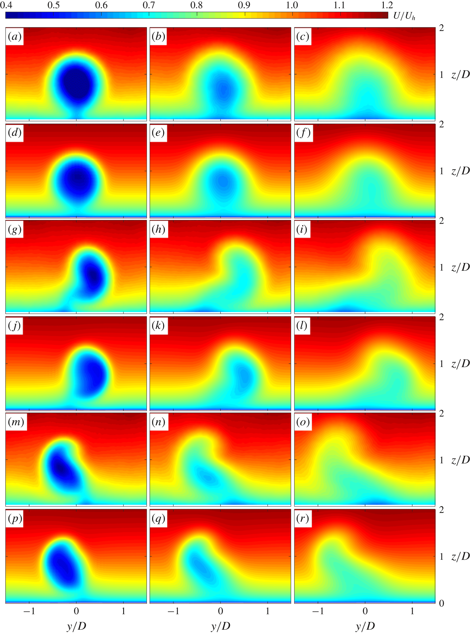
Comparison of the wake velocity contours obtained from experiments (odd rows) and the PVT model (even rows) at three yaw angles: (a–f)  $\unicode[STIX]{x1D6FD}=0^{\circ }$; (g–l)
 $\unicode[STIX]{x1D6FD}=-30^{\circ }$; (m–r)
 $\unicode[STIX]{x1D6FD}=30^{\circ }$. In each row, from left to right, the corresponding streamwise coordinates are
 $x/D=3D$,
 $6D$ and
 $10D$, respectively.

The sum of wake velocity deficit  $U_{w}$ and inflow velocity
 $U_{in}$ gives the wake velocity
 $U$. Comparisons of the wake velocity are further made in figure 7 at three different streamwise locations, ranging from the near wake (
 $x/D=3$) to the far wake (
 $x/D=10$). For all of the cases shown, the velocity contours predicted by the present model (even rows) are remarkably similar to those measured in experiments (odd rows), demonstrating that the simple point vortex transportation model proposed in this study is sufficiently accurate to reproduce the complex wake shape behind yawed wind turbines.
4.4 Validation of available power and wake centre trajectory
Based on the wake velocity shown in figure 7, the non-dimensional available power of a hypothetical wind turbine placed at ( $x_{T}$,
 $y_{T}$, 0) can be computed by equation (4.11) (Vollmer et al. Reference Vollmer, Steinfeld, Heinemann and Kühn2016). Essentially, the available power in the turbulent boundary layer without wake interference is chosen as the reference for power normalization.
 $$\begin{eqnarray}\left.\begin{array}{@{}c@{}}\displaystyle f_{AP}(x_{T},y_{T})=\left.\iint _{G}U(x_{T},y,z)^{3}\,\text{d}y\,\text{d}z\right/\!\!\iint _{G}U_{in}(z)^{3}\,\text{d}y\,\text{d}z,\\ G:(y-y_{T})^{2}+(z-z_{h})^{2}\leqslant R^{2}.\end{array}\right\}\end{eqnarray}$$
The spanwise variations of  $f_{AP}$ for three different yaw angles are shown in figure 8(a,b). At
 $x/D=3$, significant losses are observed, and the minimum available power in the wake of a non-yawed wind turbine is only 20 % of that in undisturbed flow. Yawing the wind turbine has two effects: one to shift the wake centre away from the centreline (i.e.
 $y=0$), and the other to reduce the initial wake velocity deficit by degrading the thrust coefficient by a cosine factor of approximately 1.6 (Bastankhah & Porté-Agel Reference Bastankhah and Porté-Agel2017b) and imposing less obstruction to the incoming flow. Consequently, the non-dimensional available power in the centreline is boosted from less than 0.2 to approximately 0.5. The present model slightly overestimates the available power at
 $\unicode[STIX]{x1D6FD}=0$, which can be ascribed to the ignorance of streamwise pressure gradient in near wake. Further downstream of the wind turbine at
 $x/D=10$, similar profiles of the available power are observed, and the minimum value of
 $f_{AP}$ at
 $\unicode[STIX]{x1D6FD}=0$ increases to 0.5 due to wake recovery.
(a,b) Spanwise distributions of the non-dimensional available power at (a)  $x/D=3$ and (b)
 $x/D=10$ for three different yaw angles:
 $\unicode[STIX]{x1D6FD}=-30^{\circ },0^{\circ },30^{\circ }$. (c,d) Streamwise variations of (c) the wake deflection
 $y_{d}$ and (d) the non-dimensional available power in the centreline
 $f_{AP}|_{y=0}$. The wake deflections at
 $\unicode[STIX]{x1D6FD}=30^{\circ }$ calculated from the analytical models proposed by Jiménez et al. (Reference Jiménez, Crespo and Migoya2010), Bastankhah & Porté-Agel (Reference Bastankhah and Porté-Agel2016) and Shapiro et al. (Reference Shapiro, Gayme and Meneveau2018) are plotted as thick green lines for comparison.

From the profiles shown in figure 8(a,b), the point at which  $f_{AP}$ reaches minimum can be picked. The distance from this point to the centreline (i.e.
 $y=0$), after subtracting the physical shift of the rotor centre due to yaw (i.e.
 $l_{n}\sin (\unicode[STIX]{x1D6FD})$), defines the wake deflection in this study (denoted as
 $y_{d}$). This definition of the wake deflection is directly connected to the power production and can be more robust than those determined from the middle-hub wake velocity profile (Vollmer et al. Reference Vollmer, Steinfeld, Heinemann and Kühn2016; Fleming et al. Reference Fleming, Gebraad, Lee, van Wingerden, Johnson, Churchfield, Michalakes, Spalart and Moriarty2014). The streamwise variations of the wake deflection at three yaw angles are compared in figure 8(c). The overall trends of
 $y_{d}$ are well reproduced by the PVT model, with maximum wake deflections at
 $x/D=10$ reaching approximately
 $0.4D$ for
 $\unicode[STIX]{x1D6FD}=-30^{\circ }$ and
 $30^{\circ }$. At
 $x/D\geqslant 8$, the PVT model slightly overestimates the magnitude of wake deflection, which is ascribed to the assumption of invariant vortex circulation. As explained in the last paragraph of § 4.2, due to vortex breakdown and turbulent dissipation, the total circulation of the vortex system has to decrease with downstream distance. Without taking into account this phenomenon, the transverse velocity in the far-wake region as well as the growth rate of the wake deflection will inevitably be over-predicted.
Additionally, the wake trajectories calculated from the analytical models proposed by Jiménez et al. (Reference Jiménez, Crespo and Migoya2010), Bastankhah & Porté-Agel (Reference Bastankhah and Porté-Agel2016) and Shapiro et al. (Reference Shapiro, Gayme and Meneveau2018) are also plotted in figure 8(c) for comparison. As evidenced, except for the apparent overestimation exhibited by the analytical model in Jiménez et al. (Reference Jiménez, Crespo and Migoya2010), the other two analytical models deliver satisfactory wake predictions until  $x/D\leqslant 6$. This is consistent with the results shown in Porté-Agel, Bastankhah & Shamsoddin (Reference Porté-Agel, Bastankhah and Shamsoddin2020) and to some extent expected, as the analytical models in Bastankhah & Porté-Agel (Reference Bastankhah and Porté-Agel2014) and Shapiro et al. (Reference Shapiro, Gayme and Meneveau2018) are derived, respectively, from the momentum equations and the Prandtl lifting line theory with minimal assumptions, and the major parameters are calibrated from an experimental dataset acquired in a similar condition as the current study. In contrast, during the model derivation of Jiménez et al. (Reference Jiménez, Crespo and Migoya2010), the axial induced velocity is assumed to be negligible, which can lead to large errors in the near wake.
Under the non-yawed condition, the experimental data in figure 8(c) show no evidence of wake deflection even at a distance of  $x/D=10$, which is consistent with the LES results in a neutral boundary layer presented by Vollmer et al. (Reference Vollmer, Steinfeld, Heinemann and Kühn2016). As a comparison, a non-zero wake deflection of
 $0.05D$ at
 $x/D=7$ is predicted by the PVT model. To reconcile these seemingly contradictory observations, the effects of the production/destruction term in equation (3.7), i.e.
 $W\unicode[STIX]{x2202}U_{in}/\unicode[STIX]{x2202}z$, and the top–down asymmetric distribution of the streamwise vorticity are placed under scrutiny. On the one hand, because of the counter-clockwise rotation of the wake,
 $W\unicode[STIX]{x2202}U_{in}/\unicode[STIX]{x2202}z$ is positive in the right half of the wake cylinder and negative in the left half, which helps shifting the wake centre towards the positive
 $y$-direction. On the other hand, due to wind shear and three-dimensional vortex stretching, the negative streamwise vorticity is stronger in the top-right corner of the rotor disk than that in the left-bottom corner (see figure 5a4), which, in combination with the hub vortex, induces a small negative transverse velocity in the upper half of the wake and transport the wake centre towards the negative
 $y$-direction. The net wake deflection depends on the competition of these two effects. Experimental data demonstrate that none of them wins out, whereas the proposed PVT model suggests a relatively stronger effect of the production term of the wake velocity deficit, largely because the three-dimensional vortex stretching effect is ignored and the strength of tip vortices is assumed to be independent of the phase angle, even with wind shear.
Figure 8(d) shows the streamwise variation of the non-dimensional available power along the centreline (i.e.  $y=0$). Regardless of the yaw angle, the available power exhibits an initial drop at
 $x/D\leqslant 2$ as a result of the adverse streamwise pressure gradient, followed by a gradual recovery due to turbulent diffusion. Although the present model fails to track the trend of experimental data in the near wake, accurate predictions of the available power are obtained at
 $x/D\geqslant 3$ with a mean error of less than
 $0.03$.
5 Summary
In this study, stereo particle imaging velocimetry measurements are performed in cross-stream planes at multiple streamwise locations behind a yawed miniature wind turbine (WIRE-01, diameter: 0.15 m) to reveal the physics of wake deformation and counter-rotating vortex formation. Based on these physics, a point vortex transportation model, which consists of a nonlinear transportation–diffusion equation of the wake velocity deficit and a point vortex representation of the cross-stream velocity, is derived from the momentum equations to reproduce the top–down asymmetric kidney-shaped wake of yawed wind turbines.
Both the deformation and deflection of wind turbine wakes are driven by vortex transportation. The relevant vortices include the hub vortex emanating from the rotor disk centre, and the blade tip vortices shed from the rotor disk edge. Without yaw, the streamwise vorticity shed from the rotor disk is unexceptionally negative, opposite to that originating from the hub vortex, and the net total circulation in cross-stream planes amounts approximately to zero. As a comparison, when the yaw angle exceeds a critical value, a small part of the streamwise vorticity shed from the rotor disk switches its sign as a result of the local trajectory of the blade tip vortex changing its orientation from downstream to upstream. Under mutual induction, this small part of vorticity is absorbed by the hub vortex, creating a patch of positive vorticity; meanwhile, the residual vorticity distributed along the rotor edge curls and evolves into another patch of negative vorticity. These two patches of streamwise vorticity essentially constitute the CVP and induce a top–down asymmetric cross-stream velocity field, characterized by high transverse velocity in one half of the rotor disk and low transverse velocity in the other half. Driven by this non-uniform cross-stream velocity, the initial elliptical wake is transported to one side (wake deflection) and sheared into a top–down asymmetric kidney shape (wake deformation).
The key to reproduce the kidney-shaped wake is an accurate modelling of the top–down asymmetric cross-stream velocity fields induced by streamwise vortices. Since the CVP formation of yawed wind turbines involves the hub vortex, and thus is fundamentally different from that created by a drag disk, a symmetric cross-stream velocity field derived from two counter-rotating vortices located at the top and bottom of the wake respectively becomes inadequate to reproduce the kidney-shaped wakes. In our PVT model, the cross-stream velocity field right behind the rotor disk is initialized by a cloud of point vortices with varying strength distributed along the rotor periphery, and a hub vortex located in the rotor centre. The cross-stream velocity fields at other downstream locations are obtained by simulating the time evolution of the point vortex system under mutual induction. With this model, the CVP as well as the top–down asymmetric kidney-shaped wake of yawed wind turbines can be reproduced in detail, and the available power along the centreline (i.e.  $y=0$) can be predicted with a mean error of less than 0.03.
Compared to conventional analytical models of yawed wind turbines, the PVT model proposed in this study not only captures the asymmetric wake deformation physics, but also requires no additional wake superposition laws for wind farm power prediction, largely because of its capability to model the three-dimensional flow field of an entire wind farm. Additionally, wind shear effects are already incorporated by the current version of the PVT model, and wind veer effects can be further included by superimposing a crosswind profile on the initial vortex-induced cross-stream velocity field. In future steps, the near-wake performance of the PVT model shall be enhanced by taking into account the streamwise pressure gradient.
Acknowledgements
This research was funded by the Swiss National Science Foundation (grant no. 200021 $\_$172538) and the Swiss Federal Office of Energy. In addition, this project was carried out within the frame of the Swiss Centre for Competence in Energy Research on the Future Swiss Electrical Infrastructure (SCCER-FURIES) with the financial support of the Swiss Innovation Agency (Innosuisse–SCCER programme, contract number: 1155002544).
Declaration of interests
The authors report no conflict of interest.
Supplementary movies
Supplementary movies are available at https://doi.org/10.1017/jfm.2020.123.
Appendix. Comments on the model parameters
There are four tuneable parameters in the PVT model, including the non-dimensional eddy viscosity ( $\hat{\unicode[STIX]{x1D708}}$), circulation correction factor (
 $k$), number of vortices (
 $N$) and initial vortex radius (
 $R_{i}$). Except for the number of vortices, which is an artificial numerical parameter, the other three parameters are all physics-based parameters necessary to represent the impact of ambient turbulence intensity and blade design on the wake deformation. Sensitivity analysis shows that, as long as more than 20 point vortices are used to represent the circumferential vorticity distribution, the computed wake deflection and available power differ marginally (see figure 9). For the initial radius of the tip and hub vortices, the values observed in the present experiments (
 $0.05D$ and
 $0.15D$) are recommended.
The selection of the non-dimensional eddy viscosity and the circulation correction factor desires more attention. As can be expected, when the ambient turbulence level increases, the momentum exchange rate between the wake and the free stream goes up, leading to a large value of  $\hat{\unicode[STIX]{x1D708}}$. In Niayifar & Porté-Agel (Reference Niayifar and Porté-Agel2016), LES data are used to fit a linear relationship between the turbulence intensity and the wake recovery rate. This idea can be pursued similarly in future studies, to derive an explicit expression for the non-dimensional eddy viscosity. The circulation correction factor mainly results from the fact that part of the thrust force is induced by airfoil drag and does not contribute to the generation of circulation. As such, when a different turbine is concerned, the blade element momentum theory should be employed to break down the total thrust into two parts: a lift-induced part and a drag-induced part, and the ratio of the lift-induced thrust to the total thrust can be readily used to estimate the circulation correction factor.
Variation of (a) the wake deflection  $y_{d}$ and (b) the non-dimensional available power
 $f_{AP}|_{y=0}$ with increasing number of vortices (
 $N$), at a representative yaw angle of
 $\unicode[STIX]{x1D6FD}=-30^{\circ }$.