

LINGUISTIC VARIATION AND THE INDIVIDUAL
The operating assumption of variationist sociolinguistics is that linguistic observations vary in ways that are both systematic and random. Generally, the systematic component of the observations is attributed to linguistic environments, gender, age, social class, speaking style, or other observable linguistic or social attributes of an individual. These patterns are interpreted in terms of historical processes of language change, social processes of accommodation or divergence, and so on. When observations take the form of categories, such as symbols in a phonetic transcription, we typically classify these into alternatives and analyze their distribution using logistic regression. Whereas logistic regression is common in many fields, and a standard feature of many statistical packages, variationist linguistic practice predates this, and it is more common to find linguists employing versions of Varbrul (such as Goldvarb Lion [Sankoff, Tagliamonte, & Smith, Reference Sankoff, Tagliamonte and Smith2012], the latest in the nearly 40-year lineage of Varbrul programs) for their analyses.
A criticism of variationist analysis, repeated even in its earliest days, is that it tends to elide the contributions of individuals' idiosyncrasy to the observed variation. Individuals are not treated as having distinctive contributions to variation apart from that of the groups in which they belong. A direct response to this criticism is that of Guy (Reference Guy and Labov1980), in which individual Varbrul models for individual speakers were estimated. These were painstakingly compared using a post hoc procedure to determine if individuals belonging to a common group shared the group pattern. Guy is one of a small number of researchers who continued to develop this approach in subsequent research (cf. Guy, Reference Guy1991; Guy & Boyd, Reference Guy and Boyd1990; Guy & Cutler, Reference Guy and Cutler2011; Van de Velde & Van Hout, Reference Van de Velde, van Hout., Paradis, Vincent, Deshaies and Laforest1998).Footnote 1 Current variationist practice is split. Many follow in the earlier tradition of not treating (or reporting) individual variation, implicitly treating individual variation as unimportant, whereas others see a strong role for individual variation on interpretive grounds (Bucholtz & Hall, Reference Bucholtz and Hall2004, Reference Bucholtz and Hall2005; Chambers, Reference Chambers2009; Eckert & McConnell-Ginet, Reference Eckert and McConnell-Ginet1999).
Recently, the question of individual variation has re-emerged; this time it is presented as a statistical issue wherein a different model, involving random effects for individual speaker, is presented as a more appropriate alternative (Clark, Reference Clark1973; Jaeger, Reference Jaeger2008; Johnson, Reference Johnson2009; Tagliamonte & Baayen, Reference Tagliamonte and Baayen2012). For variationist linguistics, this is the mixed-effects logistic regression model, in which a component of individual variation is estimated that is distinct from the gender, age, social class, or other group memberships of an individual. Mixed-effects models, also called random-effects models, multilevel models, and hierarchical models (Gelman & Hill, Reference Gelman and Hill2007), have been used for some time in other fields. They are related to split-plot designs for analysis of variance models, and linear regression versions are commonly used in sociology, psychology, and education, among others, to address questions for which individual variation is a concern. Logistic regression mixed-effects models are more recent, and their application is still somewhat exotic. Varbrul and its variants only estimate a fixed-effects logistic regression model; individual speaker coding is cumbersome and many analyses are run without it. Therefore, it is argued, variationist analysis using Varbrul cannot adequately address idiosyncratic individual contributions to variation, and researchers need to replace their out-of-date practice of estimating fixed-effects models in Varbrul (e.g., Goldvarb X) with a more modern one of estimating mixed-effects models using alternative software such as the lme4 package (Bates & Maechler, Reference Bates and Maechler2009) in R (Johnson, Reference Johnson2009; Tagliamonte & Baayen, Reference Tagliamonte and Baayen2012).
The criticism is a substantive one, but it makes an unfortunate three-way equation among research practice, statistical model, and software. Though we might accept the need to make some account of individual variation distinct from that of the group, it does not necessarily follow that software used in the earlier analysis is entirely inappropriate for the task. Moreover, it is not true that speaker effects must be handled as random effects, and in some research designs, it may be more appropriate to handle them as fixed effects. In this paper, I wish to show that one can model individual variation using Varbrul, in which speaker effects are treated as fixed by design. In so doing, we are able to illuminate key issues for relating statistical models to research design, which in turn argue against uniformly recommending random effects for modeling individual speaker variation as suggested by Johnson (Reference Johnson2009) and Tagliamonte and Baayen (Reference Tagliamonte and Baayen2012).
This argument is presented in two major sections. In the following section, the mathematical side of the argument is presented, in which a general model statement allows us to relate the mixed-effects model to the individual-level models of Guy (Reference Guy and Labov1980, Reference Guy1991, etc.) and the traditional type of Varbrul model, without individual effects. A fourth type of model, the speaker fixed-effects model is presented as an alternative. The subsequent section presents a worked example involving was/were variation data in York English (Tagliamonte, Reference Tagliamonte1998; cf. Tagliamonte & Baayen, Reference Tagliamonte and Baayen2012), in which different but related models are estimated from identical data, to highlight the different consequences of different starting assumptions. This is followed by a discussion underscoring the relationship of these different assumptions to different research designs. Hence, the conclusions we draw regarding individual variation are related directly to the assumptions we make in our analysis, which in turn need to be dictated by the specification of the research design. This conclusion is methodological, rather than substantive, and so applies broadly to linguistic variation research, indicating a need to clarify research designs and starting assumptions―in particular those about sampling and the nature of speaker-specific variation as well as more technical ones such as optimal model search criteria―when presenting statistical models of variation.
MODELING VARIATION
The model behind the Varbrul family of programs is the logistic regression model, which may be stated as in Eq. (1), in which the logit (log-odds) of a probability is predicted as an additive combination of a number of terms: an overall rate of variation a (input in Varbrul parlance), one or more terms b nx n representing the product of a predictor variable (factor) x n and its associated effect parameter b n, (or factor weight) and an error term for individual observations e (Paolillo, Reference Paolillo2002; Sankoff, Reference Sankoff1978).
 $$\ln \lpar p/\lsqb 1 - p\rsqb \rpar = a + b_1 x_1 + b_2 x_2 \ldots + e \eqno \lpar 1\rpar$$
Equation (1) is used as follows. We begin with a set of observations of the rate of use p of some linguistic variable, classified according to the different values of the contextual variables x 1, x 2, and so on. The estimation program (e.g., Goldvarb) searches for suitable values for b 1, b 2, and so on, that give a good fit to the observations when Eq. (1) is used to predict them. The criterion of fit is the log-likelihood of the model, computed by comparing observed and expected counts in each cell (i.e., each unique combination of factors), and summing over all cells; the log-likelihood is also used to compute G 2, a chi-squared distributed statistic, for significance tests.Footnote 2 Most versions of Varbrul use a variant of iterative proportional fitting ([IPF] Bishop, Fienberg, & Holland, Reference Bishop, Fienberg and Holland1975) for estimating the b n values.Footnote 3
An assumption implicit in the model in Eq. (1) is that all of the effects b n are “fixed” by design. Effectively, this means that the researcher has chosen speakers, for example, to use because of the factors x n they exhibit, and that the observations are not correlated by any unanalyzed factor, such as individual speaker. The research goal is finding the appropriate set of factors x n to use in describing the variation observed, and stepwise selection of predictors (step-up/step-down analysis) is commonly used to eliminate nonsignificant factors—those that fall below a significance threshold in their effect on the rate of linguistic variable use. Alongside this, speakers are usually treated only in aggregate according to their demographic characteristics and are not treated as having potentially different individual patterns of variation.
The problem, however, is that observations from the same individual are actually correlated and can be expected to be more like each other than they are to those of another individual. Correlated observations tend to give the appearance of smaller variance within the group categories than should actually be there, and consequently, group effects are more likely to appear significant. To address this problem, a different type of model is used, known as a mixed-effects model. This model has a variety of different possible statements, one of which is Eq. (2) (see Kreft & de Leeuw, Reference Kreft and De Leeuw1998:22, for a similar statement of mixed-effects linear models).
 $$\ln \lpar p\lsqb 1 - p\rsqb \rpar = a + b_f x_f + c_s + d_{fs} x_{fs} \ldots + e \eqno \lpar 2\rpar$$
This model statement adds two extra terms to the one in Eq. (1) to address the question of speaker effects. As before, a represents the intercept, whereas b fx f represents a linguistic or social factor (fixed) effect (as before, there may be other b nx n terms representing different relevant factors). The term c s represents an overall rate for each individual speaker; essentially, each speaker has her/his own intercept, expressed in terms of how it is different from the overall intercept (cf. Drager & Hay, Reference Drager and Hay2012). Similarly the d fsx fs term represents each speaker's own factor effect, that is, how that speaker's factor effect differs from the one for the sample as a whole. Because our goal is to make inferences about what typical people would do, we regard the individuals as if they were sampled from the larger population; hence, speaker is treated as a random variable, and the parameters representing speakers' properties vary like random variables. For this reason, the parameters c s are often called random intercepts and d fs are called random slopes. As random variables, we expect them to be normally distributed, allowing c s and d fs to be characterized using their standard deviations. This results in a simple model with only one parameter for each random effect, instead of one per speaker for each. The model in Eq. (2) is harder to estimate than that in Eq. (1) is; various R (R Core Development Team, 2010) packages are typically recommended for such models, such as nlme or lme4 (Bates & Maechler, Reference Bates and Maechler2009; Pinheiro, Bates, DebRoy, Sarkar, & the R Core Team, Reference Pinheiro, Bates, DebRoy and Sarkar2009). Stepwise regression, though a built-in feature of Goldvarb, is deprecated in the mixed-effects modeling context (Gelman & Hill, Reference Gelman and Hill2007); instead, all significance tests are based on the full model—the one with the maximal set of factors in place—giving a stricter test. Speaker-level effects are not subject to significance testing, as they are characterized by an independent population model.
The complaint against variationist analysis using Goldvarb thus boils down to this: The model employed by Goldvarb is a fixed-effects only model, which does not partition the variation into components representing individual-level variation (random intercepts) and group-individual differences (random slopes). Because the observations made are correlated within individuals, our estimates of group effects are inflated and, hence, significance tests in Goldvarb (or other fixed-effects approaches) are inflated. We will, in other words, find group effects where there are none to be found, and all of the variation observed should be accounted for at the individual level.
The logistic regression model in Eq. (1) is actually a fairly simplistic application, which does not assume interaction effects. One type of interaction leads to models called hierarchical models, in which certain factors are “nested” within other factors. Hierarchical models have a close relationship to mixed-effects models. We will consider here a hierarchical, speaker fixed-effect model, wherein speakers are nested within groups. This arrangement expresses exclusive group membership (e.g., speakers belong to only one gender);Footnote 4 significant differences between groups are identified when speaker variation within groups is more homogeneous than across groups. Careful handling of significance testing and model reporting permits the model to compare closely to mixed-effects models. This approach provides rich and interesting information regarding language variation, where inflated significance tests have been appropriately guarded against.
Consider again the model of Eq. (2), which has the terms a, b fx f, c s, and d fsx fs. Using a different notation, we can write these terms as main and interaction effects in a logistic regression model. We use dot notation, in which all parameters have two indices, for group and speaker, respectively, and a subscript dot (•) means that that particular parameter value is the same for all values of the respective index. The model is now expressed as in Eq. (3). We also invoke explicitly different variables x s for subject and x f for linguistic or group factor; these have only one index each.
 $$\ln \lpar p\lsqb 1 - p\rsqb \rpar = a_{ \bullet \bullet } + b_{\bullet s} x_s + b_{f \bullet} x_f + b_{fs} x_f x_s \ldots + e \eqno \lpar 3\rpar$$
In this model statement, the parameter a •• is equivalent to the intercept parameter a in Eq. (1); it expresses an overall rate of variation, and the same value is used for all speakers and groups. The parameter b •s applies to all levels of factor f but varies specifically according to each speaker; this parameter expresses the way the intercepts of individual speakers differ from a ••, just as c s expresses speaker differences from a in Eq. (2). Formally, this is a main effect parameter, because it has only one nondotted index. The variable x s in this term represents explicitly a speaker factor identifying each speaker in the pool. The parameter b f• in the term b f•x f varies by factor, but it applies to all speakers; it represents the main effect for group independent of speakers' idiosyncratic variation and corresponds to b fx f in Eq. (2). Finally, the parameter b fs in the term b fsx fx s varies by both speaker and group; it corresponds to d fsx fs in Eq. (2) and is formally a factor-individual interaction parameter. Both speaker and factor variables are involved in this term. By labeling all of the parameters in Eq. (3) as b and providing the appropriate indexes, we make explicit their relationship to the model in Eq. (1), while the subscript indices indicate how the variables and parameters need to be composed to obtain a model with term-for-term parallels to that of Eq. (2). Note that if x f is a linguistic factor, so that it appears for all individuals, the number of parameter values in b fs equals the number of factor levels times the number of individuals. Conversely, if it is a group factor in which speakers belong to one and only one group, then the term b fsx fx s will have no meaning, because all of its values will be zero. (Values of b fs where individual is paired with a nonmatching group will be zero, because speakers can only be in one group. Values of b fs where speaker matches its group will also be zero, because they are redundant with b •s.)
Models with interaction terms like those in Eq. (3) are commonly used in logistic regression, and Goldvarb provides facilities for specifying them via recoding conditions files. Goldvarb (and other variants of IPF) reliably estimate such models as long as they follow the hierarchy principle (Bishop et al., Reference Bishop, Fienberg and Holland1975:67), which prohibits a higher-order parameter (e.g., b fsx fx s) from being included in a model unless a corresponding lower-order parameter (e.g., b sx s) is also included; in this arrangement, the higher-order effect is said to be “nested” within the lower-order effect. In fact, this is exactly the circumstance indicated in Eq. (3), and it is from this hierarchy principle that mixed-effects modeling gets the alternate name hierarchical modeling. Accounting for nested, hierarchical effects in a research design is an important role of mixed-effects modeling, especially in social science research (Kreft & De Leeuw, Reference Kreft and De Leeuw1998:3–8); the fixed-effects version employing interactions is thus a competing but closely related account.
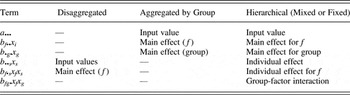
Table 1 summarizes the correspondences between terms in three types of models: disaggregated by individual (e.g., cf. Guy, Reference Guy and Labov1980); aggregated by group (i.e., as in Eq. (1)); and hierarchically nested speakers within groups, as in Eq. (3). For completeness, we include one group factor x g and one linguistic factor x f, meaning that parameters will have three subscripts for linguistic factor, group, and individual, respectively. Most realistic models have multiple linguistic factors and multiple group factors (possibly involving other levels of nesting), and the number of subscripts would have to be increased to fully represent such models in this notation.Footnote 5 The full set of terms for this relatively simple model—including intercept; main effects; one-, two-, and three-way interactions—is listed in the first column of Table 1. Cells in which a dash is present indicate that that term is missing from the model (i.e., the corresponding b is set to zero).
Corresponding terms in three models: Disaggregated by individual, aggregated by group, and hierarchically nested (individuals within groups)

In Guy's practice of disaggregating by speaker (e.g., Guy, Reference Guy and Labov1980), there are input values (intercepts) and main effects for each individual speaker. There are no overall input values or main effects, however, because the speaker models are estimated independently. Moreover, questions regarding the relation of the individual to the group, or the group and the linguistic factor, have to be handled by post hoc interpretation, as there are no model terms representing these effects. The input values and (linguistic) main effects of the individual models are thus more complex terms, because they are conditioned on the individual. The practice of aggregating by group lacks any terms for individual effect, for the same reason.Footnote 6
In contrast, the hierarchical model includes terms corresponding to those of both the other types of models; its main effects are interpreted as the main effects of the aggregated model would be, but without the hazard that the individual effects have been ignored. The individual effects are interpreted as the main effects of the disaggregated models would be, but without requiring a post hoc procedure for interpreting group main effects. The model also potentially includes interaction effects, corresponding to observations such as the differing weighting of final consonant and word boundary as (t/d)-deletion environments among speakers of Philadelphia and NYC English (Guy, Reference Guy and Labov1980). Furthermore, group and individual effects appear together in the same model, raising the possibility that both can be tested for significance.
It is in this respect that the models in Eqs. (2) and (3) differ most. There is no probability model in Eq. (3) that applies to the speaker-varying parameters as it does in Eq. (2) and no one-parameter representation of the random effects. At the same time, the probability model over b s values posited for Eq. (2) prohibits significance testing of the individual effects. Individual effects are simply assumed and characterized by their observed empirical distribution. If the sample of individuals is nonrandom, this characterization would be in error. In contrast, speaker effects in Eq. (3) have the same status as all the other model parameters and can be individually or collectively tested for significance. Doing so implies different assumptions about the nature of interspeaker variation from those of the random-effects model. Most importantly, individual speakers are treated as fixed by design, and their parameter values are not regarded as being necessarily representative of variation across speakers generally. Interspeaker variation is thus treated as an open hypothesis, with the same status as variation at the group level.
Furthermore, the search for an optimal model can be adapted toward practices of mixed-effects modeling, for example, by adopting the stricter practice of conducting significance tests beginning with the full model. For this approach, all of the necessary tests are found in the stepping-down phase of Goldvarb's stepwise analysis, so software itself is not an obstacle, merely the interpretation of the output. Admittedly, many tests unnecessary for this comparison are run in both the stepping-up and stepping-down phases, but a manual procedure can also accomplish the same thing. One can also manually estimate a probability model post hoc over the b •s and b fs parameters. This is similar to what is done in a mixed-effects model and a close approximation of hierarchical modeling practice before special software became available (Kreft & De Leeuw, Reference Kreft and De Leeuw1998). Hence, the model in Eq. (3) is at least a good starting point to better understand the issues involved in modeling individual variation and comparing it to more traditional modes of variationist analysis.
A SPEAKER-LEVEL ANALYSIS OF WAS/WERE VARIATION IN YORK ENGLISH
We now turn to a concrete example of analyzing individual variation using a hierarchical speaker-effects model based on data provided by Tagliamonte from her study of was/were variation in York English (Tagliamonte, Reference Tagliamonte1998); a related but nonidentical corpus is used in a restudy using a mixed-effects model in Taglaimonte and Baayen (Reference Tagliamonte and Baayen2012). Standard English requires was with first- and third-person singular subjects and were with second-person and/or plural subjects, although nonstandard was with second-person or plural subjects, as well as were with first- and third-person singular subjects, are commonly observed in many varieties of English. In the 1998 study in York, England, speakers were classified according to age and gender, for which it was argued that women had greater frequencies of nonstandard variants than men did, and older and younger age groups also had a greater frequency of nonstandard uses than the middle-age group did. Linguistically, negative contexts (e.g., wasn't, weren't) appear to show greater nonstandard usage than affirmative ones do.
Because many different individual speakers may be involved in a given variationist study, there will typically be large numbers of codes in the speaker variable and consequently in any speaker-group interaction. Disaggregating data by speaker also places special requirements on data balance across speakers and linguistic contexts (cf. Guy, Reference Guy and Labov1980). Essentially, we partition the dataset into individual speakers and run similar analyses on each speaker, with group-level results coming from a comparison across speakers. For that to work, we need enough data from each speaker to support a full variable linguistic analysis. The number of tokens required depends on the number of parameters being estimated and the number of linguistic contexts the data are broken into, but generally, 100 tokens per speaker is a minimum to ensure reliable estimates. Overpartitioning the data is a potential concern (Long, Reference Long1997; Paolillo, Reference Paolillo2002:135), and care must also be taken to prevent poorly considered variables from leading to problems with convergence.
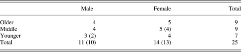
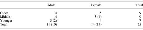
In the data available for restudy, there were 46 speakers, with a total of 6809 tokens of was/were (5150 was, 1659 were), but 21 of these had fewer than 100 tokens of the was/were variable and could not be included. Of the remaining 25 speakers, 14 are women and 11 are men; 9 are in the older age group (over 65 years old), 9 are in the middle age group (35 to 65 years), and 7 are in the younger age group (under 35 years); and speakers are relatively balanced by the age and gender categories, at least given these numbers of overall speakers (see Table 2). The analyzed portion of the corpus contains 5801 total tokens, 4595 of which are instances of was, and 1206 of which are instances of were. Two speakers, one younger man whose was/were use was categorically standard, and one middle age-group woman whose was/were had categorical was in standard was contexts, had to be excluded from the variable linguistic analysis because of knockouts.
Distribution of speakers in the analyzed portion of the York corpus, by age and gender
The corpus was originally coded for a number of linguistic features, including sentence polarity (affirmative versus negative); standard was versus standard were contexts (i.e., first- and third-person singular versus second-person and/or plural subjects); copula versus auxiliary function of was/were; contracted versus full form; noun phrase (NP) complement (or object) type (12 categories); lexical noun type (62 categories); determiner type (strong, weak, and other); syntactic configuration (10 categories); syntactic configuration of the object/complement NP (12 categories); syntactic proximity of the closest NP to the verb (8 levels); number of proximate subject or nonsubject NP (4 categories); and occurrence of a nonexistential, postposed NP (2 categories).
Though each of these factors represents a reasonable hypothesis about the distribution of was/were (in terms of having support in the research literature), they did not show strong effects for the York corpus in earlier research (Tagliamonte, Reference Tagliamonte1998). Inclusion of them in the current research would complicate the design, by compounding the data partitioning problem. Had the full complement of variables been considered, none of the speakers would have had sufficient data to justify an analysis. Here we focus on a subset of the coded features that make the strongest methodological demonstration. We will come to see that the data do not strongly determine the results of the statistical analysis and that certain assumptions, the selection of which should be guided by the research design, are every bit as important.
The present example focuses only on two speaker group variables—gender (2 categories) and age (3 categories)—and two linguistic context variables—standard and nonstandard environments (2 categories) and positive and negative sentences (2 categories). This leaves a relatively modest number of parameters to be estimated for each speaker (intercept + context + polarity = 3), and an adequate number of cells (4) and observations (from 110 to 485 per speaker) to compute them. For 25 speakers, we have a total of 75 parameters. The individual speakers are distributed across 3 ages and 2 genders, or another 6 cells, from which we hope to estimate 4 additional parameters for age, gender, and overall rate (i.e., the intercept) effects. Without other interaction effects, this means that the model we are seeking has potentially as many as 79 parameters, with observations in 100 cells, leaving 21 residual degrees of freedom.Footnote 7 This is a large number of parameters, probably larger than that found in most variationist applications of logistic regression, but, at the same time, the model is not overspecified, and, with the right kind of care, we should be able to estimate it and test each of the factor groups for significance. Note that a mixed-effects model has a similar complexity (Baayen, Davidson, & Bates, Reference Baayen, Davidson and Bates2008). Although fewer parameters are used, the values of the random speaker variables have to be estimated so their true cost in degrees of freedom is similar.
RECODING FOR HIERARCHICAL MODELING
Recoding a dataset to use a hierarchical speaker-effect model in Goldvarb requires use of the conditions file syntax, a LISP-based sublanguage in Varbrul programs (Rand & Sankoff, Reference Rand and Sankoff1988). This feature is somewhat richer than is strictly necessary for the operations involved. In other software (e.g., SPSS or R), equivalent operations can be done either by specifying appropriate interaction terms in a model or by using other recoding facilities. Details of these operations will vary considerably, so the example here addresses only what needs to be done when using Goldvarb. For example, in R and SPSS, to obtain the correct model parameterization, one would need to specify contrast functions for the appropriate variables, because default contrasts result in reference-cell parameterizations (see Paolillo, Reference Paolillo2002:166–169), resulting in unhelpful significance tests and complicating interpretation (contra Tagliamonte & Baayen, Reference Tagliamonte and Baayen2012:149). Goldvarb only uses difference-between-means parameterizations, and it is unnecessary to invoke a special command or function to achieve the desired result.
The conditions file for a hierarchical speaker-effects model needs to keep the individual speakers distinct while assigning them to appropriate groups. At the same time, it must distinguish the linguistic environments for variation within each speaker. Employing a speaker variable with a distinct code for each speaker, so that the speaker who produced each observed token is known (as recommended in Tagliamonte, Reference Tagliamonte2006:123) is enough to obtain a speaker fixed-effect model that corresponds closely to the random-intercept model for speakers, although one can also code speakers into specific groups using the exclusion operator, written with the slash character ‘/’. Using this strategy, we can code speakers into six groups (younger, middle, and older women; younger, middle, and older men), where in each group, the three to six speaker identities are kept separate and all other speakers are excluded from the group. The difference-between-means parameterization computed by Goldvarb centers parameter weights on the mean for the group, but they are weighted according to the quantity of data for each individual. When a group-effect is present in the model, it is centered on the mean for all the groups; such an effect will be significant only if differences between group means overwhelm the speaker-specific variation within each group. Splitting the speaker-specific variation by group also has the practical benefit of making it easier to recognize which speakers are which in a model that has many speaker-specific effects.
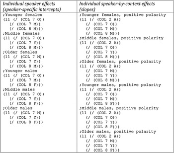
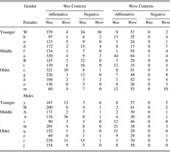
As implied by Eq. (3), individual effects for linguistic factors are incorporated using interaction coding techniques, where each linguistic context is represented as an interaction effect with speaker. This ensures that speaker-specific effects will always be taken into account when estimating linguistic factor effects. As before, we can test within-group variation for significance more conveniently when speakers in each of the different groups are coded separately. In other words, just as with the group effects, we need an aggregate context effect and individual context effects for each speaker. The only difference in this case is that individual speakers are not “assigned to” one and only one linguistic context, as they are in the case of social group variables. The context variables, in other words, cross the speaker variable, rather than partition it. This recoding can also be accomplished using the exclusion operator to delete tokens corresponding to the appropriate context. The full set of operations is illustrated in Figure 1, and the resulting frequencies of was and were for each of the factor combinations are given in Table 3.
Recoding subject into individual and interaction effects, gathered into six groups, for the York English corpus. The exclusion operator (/) is used to drop tokens corresponding excluded factor values. Remaining tokens are coded and aggregated according to the values in group 11, which represents individual speakers in this example.

Cross-tabulation of was and were instances by individual speaker, in affirmative and negative sentences, standard was and were contexts

Note: Men and women are separated; within each gender, three different age brackets are indicated.
By using the recoded variables together in an analysis, we obtain estimates for individual speaker effects (the b •sx s of Eq. (3), corresponding to the “random intercepts” of Eq. (2)) alongside the group main effect parameters (the b g•x g of Eq. (3)). When the group main effect is tested for significance, it is done in the context of a collection of individual effects that are independently estimated. It is also possible to test the individual effects for significance this way, something that cannot be done in the mixed-effects framework. Note that because different groups are specified separately, we do not need to assume that male and female intercepts have a common variance; for example, it would be possible for (some) men, but none of the women, to test as significantly different from their group. This means that a rich range of interaction structures can be considered using this single coding. Comparable analyses could not be run as mixed-effects models without additional steps.
Significance testing of the effects in a hierarchical speaker-effects Goldvarb model is handled using the likelihood ratio chi-squared (or G 2) test (Agresti, Reference Agresti1996; Bishop et al., Reference Bishop, Fienberg and Holland1975), which is a comparison of the likelihood of two models. This is the same criterion implemented in the step-up/step-down procedure of Goldvarb, so all required significance tests can be done automatically. Whether this is practical or not depends on the number of factor groups, because many tests are conducted that will simply not be used (i.e., all of the stepping-up tests). The runs that are relevant depend on what assumptions the researcher employs. For exploratory analysis assumptions, as in usual Varbrul practice, the step-up/step-down procedure is interpreted as it normally is, that is, the “best” models from both stepping-up and stepping-down are compared and the best-fitting one is interpreted (in the ideal case, the two are identical). For mixed-effects model assumptions, which dictate that any potential sources of variation in the data be retained in the final model (Gelman & Hill, Reference Gelman and Hill2007:271), all of the significance tests can be found in the first stepping-down level, starting from the full model (this corresponds to backward elimination stepwise regression in many other regression programs).
RESULTS OF THE HIERARCHICAL ANALYSIS
Two analyses were run using the coding described herein. In the first analysis, the full model was used to obtain parameter estimates for each of the individual, group, and contextual factors in the model. Significance tests were conducted by excluding factor groups one at a time: one separate run for each factor group for a model corresponding to the full model minus that specific factor group. The model log-likelihoods were compared to the full model using the likelihood ratio test to arrive at a p value for each factor group. Speaker-specific effects were treated as though they were coded in a single factor group; that is, in each model either all speaker intercepts were included or none, either all speaker-context effects were included or none, and so on. This way, an analysis that comports with the assumptions of mixed-effects modeling was conducted, with the remaining differences being the treatment of the speaker effects as fixed. The second analysis was conducted in the usual way, using Goldvarb's step-up/step-down procedure. This analysis was meant to compare the results of the usual exploratory analysis procedure of variationist analysis with those of the hierarchical analysis.
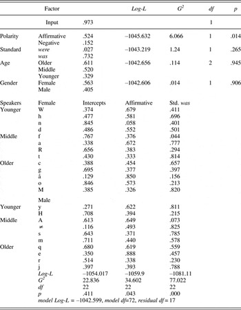
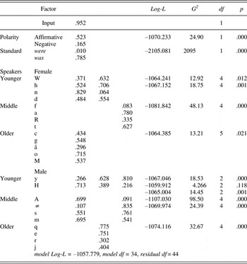
The first analysis is presented in Table 4, where for each factor group, there are factor weights representing each factor, and a log-likelihood (Log-L), G 2, degrees of freedom (df), and p value for the group as a whole. The speaker-specific effects are presented in three columns (intercepts, affirmative, and standard was), with the factor group summary statistics at the bottom of the corresponding columns. Using p ≤ 0.05 as the significance criterion, the following factor groups are significant: a main effect for polarity, and specific speaker effects for affirmative and standard was contexts. Main effects for age, gender, and standard was/were are nonsignificant, as is the speaker-specific intercept.
Hierarchical model of York was/were variation

It appears that speakers do not vary much in their overall rates of was/were use (the intercepts), although they do differ from one another in the affirmative and standard was contexts. For the affirmative context, this variation is systematic, such that negative sentences are less likely to show was than affirmative contexts are. Speakers' variation in was/were realization across standard was/were contexts is not systematic in this way. Apparently, speaker variation is also not systematic by demographic group (age and gender), as these main effects are not significant. Either we do not have demographic categories that reflect the variation in was/were, or our sample of speakers is too small to reveal systematic variation that exists. Unfortunately, this model does not let us speak to this question.
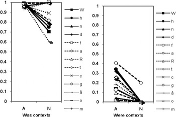
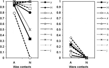
To verify the patterns observed in the model, the rates of was/were observed in each of the different contexts (Table 3) were plotted by speaker, in four interaction plots: female speakers in standard was and were contexts in Figure 2, and male speakers in standard was and were contexts in Figure 3. The x axes in all four charts distinguish the affirmative (A) and negative (N) contexts. Note that because negative contexts are far less frequent than the affirmative ones are, the overall number of observations for these proportions is far smaller, especially in the case of the standard were contexts, which are also fewer in number than standard was contexts. Figures 2 and 3 exhibit similar patterns: for both men and women, there is greater variation in was use in the negative/standard was contexts and in the affirmative standard were contexts. Although the age groups are indicated by line quality, no clear pattern emerges in the interaction plots for the different age groups. For example, the middle age group (dashed lines) appears at both extremes for men in the standard was contexts. Across the two figures, it appears that men may have a greater range of variation in the standard was contexts, whereas women may have a greater range of variation in the standard were contexts. This apparent interaction was not tested in the model of Table 4. The evidence for significant speaker-specific variation in the pattern observed in the model is not resoundingly strong either, although the interaction plots can be read as showing greater interspeaker variation in affirmative and standard was contexts.
Proportion of was variant among female subjects, standard was and were contexts, in affirmative and negative sentences. The three age groups are indicated by solid (younger), dashed (middle), and dotted (older) lines.

Proportion of was variant among male subjects, standard was and were contexts, in affirmative and negative sentences. The three age groups are indicated by solid (younger), dashed (middle), and dotted (older) lines.

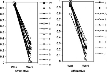
However, these observations must be interpreted with caution, because the data representing the negative contexts is quite limited (see Table 3), and the scale of the plots is in proportions rather than logit units in which the model of Eq. (3) and Table 4 would be linear and additive. In all four plots, the affirmative standard was contexts and the negative standard were contexts are nearly categorical, regions where the logit transform is most nonlinear. Hence, the scale of the plots is severely distorted in these regions. Interaction plots of the affirmative contexts only help to emphasize this point; these are the contexts for which the data quantity is greatest, and the parameter estimates are more robust. These are given in Figure 4 for female and male speakers, and it is clear in these plots that the standard was/were context has the greatest influence on the occurrence of was, although there is interspeaker variability with respect to how much variation is seen. Again, female speakers appear to show more categorical use of was in standard was contexts, but this could still be an effect of distorted scale. Note also that the appearance of greater variance in standard was contexts may be due to a single man from the middle-age group.
York women (left) and men (right) in affirmative standard was and were contexts only. The three age groups are indicated by solid (younger), dashed (middle), and dotted (older) lines.

RESULTS OF STEPWISE EXPLORATORY ANALYSIS
A stepwise analysis was conducted for this dataset using Goldvarb's step-up/step-down analysis procedure. The complete procedure took nearly 18 hours on a MacBook Air 1.1 laptop with an Intel Core Duo 2 processor.Footnote 8 Most of the models failed to converge after 20 iterations, hinting at potential shortcomings in Goldvarb's use of IPF. However, both directions of stepwise model selection selected the same final model, given in Table 5, so there does not seem to be any need to criticize the lack of convergence of parameter estimates too strongly. The significance tests reported in Table 5 are taken from the models in the final stepping-down level, where each test represents a model comparison between the final model and one with a particular factor group excluded. This corresponds to the stepwise elimination tests based on the full models as used in Table 4, but where instead of the full model, the final stepwise-selected model is used for comparison. In one factor group, the younger man by affirmative speaker-specific factors, it appears that Goldvarb is not correctly counting degrees of freedom for groups coded with the exclusion operator; in this case, the df that should be used is 2 (one parameter for each speaker), because the factors in this group do not fully cross all of the other contexts, as they do when the full set of speakers is given speaker-specific factors. When the incorrect df, 1, is used, the G 2 value appears to be significant (p = 0.039).
Stepwise selected best model of York was/were variation

The selected model is more parsimonious than the model in Table 4. It has 34 parameters accounting for 78 cells (44 residual df) instead of 72 parameters accounting for 89 cells (with 17 residual df). Moreover, the likelihood ratio of the two models is not significant at the difference in residual df of the two models (G 2 = 30.36, df = 27, p = 0.298). There is a clear descriptive economy for the stepwise-selected model over the hierarchical model in Table 4.
The model in Table 5 also fits our reading of Figures 2 to 4 a bit more closely than the model in Table 4 does. It has main effects for the standard was/were context (the strongest effect, in terms of its influence on log-likelihood) and polarity. Among the speaker-specific effects, a large number are shown to be nonsignificant, although there is no clear pattern in the selection among the different groups. Younger men and women, middle-age men, and older women have significant speaker-specific intercepts, whereas in affirmative contexts, younger women and men are significant. In the standard was contexts, middle-age men and women and younger men are significant. Evidently, there is enough interspeaker variation among them to justify the additional parameters that they require. To interpret them, we need to explain why those particular groups show greater interspeaker variation than others do. This is at best a speculative exercise for someone not closely familiar with the individuals and the contexts of data collection.
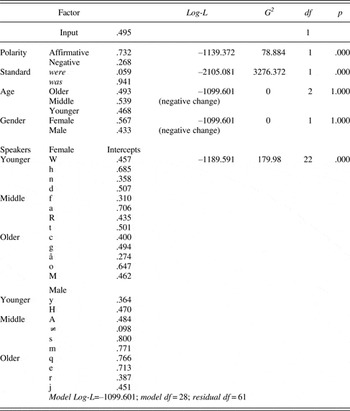
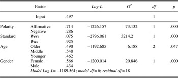
To complete our comparison of models, we need to consider two more models: a model with speaker intercepts only, similar to the model used by Drager and Hay (Reference Drager and Hay2012), and a model with no speaker effects, reflecting more traditional variationist practice. The speaker-intercepts model might be used when accounting for speaker-variation is a concern, but random slopes would overpartition the data. These two models are presented in Tables 6 and 7, respectively.
Speaker intercept model of York English was/were variation

Best model, by traditional assumptions, of the York English data with identical speaker subset as previous models

The speaker-intercept model in Table 6 and the main-effects model in Table 7 have strong similarities to the models in Table 4 and Table 5. All of the effects except for age show similar weights across the models (in spite of the fact that the overall intercepts [input values] are different). Age appears to be the least significant factor group, so it is not entirely surprising that the rank order of the factors by weight changes from one model to the next. These effects are not altogether very strong. Speaker intercepts are not consistently rank-ordered by weight across the models in Tables 3, 4, and 5, but within age-by-gender groups, the order is maintained more often than not.
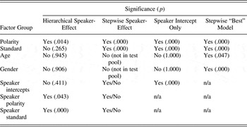
Some of the values of the speaker intercepts also change across the different models. The difference between models in Tables 4 to 6 has to do with the inclusion or exclusion of interaction terms from the model, so their main effect terms also look very different. Consequently, the disaggregated model (Table 6), without the interaction term, appears least trustworthy. We note, however, that this appears to affect only the least significant of the main effects (age), and that the models in Tables 4 through 7 are otherwise similar to one another in terms of the values of their parameter weights. What is different across the models is the significance attributed to the G 2 tests, and the assumptions of those tests. Table 8 summarizes the results of these tests, and the assumptions under which they were conducted.
Significance of different factor groups and test assumptions in each model

Polarity shows up as the one factor group whose main effect is significant across all of the models, in spite of the fact that the charts in Figures 2 through 4 make clear the significant role of standard/nonstandard was/were contexts. It appears that the peculiar nature of the polarity-by-standard interaction is such that there is greater interindividual variance for negative sentences in standard was contexts and for affirmative sentences in standard were contexts. The high interindividual variance, coupled with the low numbers of observations of negative sentences, results in a nonsignificant main effect for standard was/were context, where it looks like it should be significant. It appears that the significance test might be too strict in this case.
Although speaker-polarity and speaker-standard effects are significant, the intercepts are not significant in the final model (Table 4). It is difficult to interpret this, however, because the significant effects do not appear to pattern in terms of the known demographic characteristics of the speakers. Moreover, hierarchical modeling assumptions would not permit us to interpret them, because they would be taken to represent a population and used to estimate the parameters of the population model. The parameter values in the three speaker groups here could be given for a population model that specifies, on the logit scale, means of zero and standard deviations of 1.066, 1.042, and 1.462 for intercepts, polarity, and standard was/were, respectively (on the probability scale these are .743,.739, and .811). This tells us little that is interpretively useful, other than that the speaker effects can vary over nearly the entire probability range using a 95% confidence interval.
The stepwise speaker-effect model spares us the potential embarrassment of lacking a significant main effect for standard was/were context. The tests responsible for rejecting age and gender as significant are not necessarily found in a single run that gives the significance for the other factor groups, though they can be retrieved from the stepwise analysis at different points. Care needs to be taken in interpreting these tests, because the significance tests in Table 5 represent a level of aggregation that does not take gender and/or age into account, so the entire set of tests are not commensurate. Moreover, Goldvarb's stepwise analysis uses relaxed assumptions regarding significance testing in comparison to hierarchical modeling. Significance testing of speaker-specific effects is a part of this second model, although there is no guarantee that any interpretable pattern of significant effects emerges. Also, there is an evident trade-off in the significance of the standard was/were main effect and that of certain speaker effects (and their consequent exclusion from the model). Hence, aggregations across different models (and across speakers) appear to be inconsistent, and the entire stepwise testing procedure could be held suspect on these grounds.
Similar observations can be made for the third model (Table 6), which considers only speaker-specific intercepts. In this model, speaker-by-polarity and speaker-by-standard was/were context effects are excluded from consideration a priori. With this sole exception, the assumptions regarding significance testing are the same as for the hierarchical model. Various justifications for this relaxation of assumptions can be given, but the considerable degrees of freedom freed from this, and the consequent aggregation across speakers clearly permits significant main effects for both polarity and standard was/were context to be found, suggesting the interpretation that in York English polarity competes with agreement for was/were marking, but without any suggestion as to the source or direction of this dialect feature. The difference between significant and nonsignificant factor groups is very sharp (the nonsignificant ones result in a negative change in log-likelihood, i.e., worse model fits when excluding the tested group).Footnote 9
The final model, the “best model” under usual variationist assumptions, which excludes consideration of any speaker-specific effects, continues the pattern we have seen. Relaxed assumptions (regarding the relevance of speaker-specific effects) permit more factor groups to be found significant. Note that the age factor group, with a significance level of .047 would customarily be interpreted. However, when compared with the other models, which all find age to be nonsignificant, this is an unsafe conclusion to make. The probability level observed is just shy of the criterion value (and nowhere close to it in the other comparisons). This would appear to be a case of either inflating the significance of a result due to greater available degrees of freedom or simply improper aggregation as a result of excluding factors in the stepwise analysis.
DISCUSSION
We now return to the questions of accounting for individual variation in variationist research. First, is Goldvarb up to the task? Here the answer is yes. There is no insurmountable obstacle to using Goldvarb for estimating models with speaker-specific effects. A broad range of models with speaker-specific effects can be considered and evaluated against one another, so long as they are properly specified. The only difficulties encountered when employing Goldvarb this way are (i) complexity of coding, (ii) problems with nonconvergence, (iii) incorrect degrees of freedom being used in certain tests, and (iv) significance testing from different models with incommensurate and potentially improper aggregations.
The first problem is likely to exist in some form for any model in which a factor group with many levels is required, such as speaker, regardless of what software is used for estimation. The second issue could be addressed by adopting a different estimation algorithm instead of IPF with better convergence properties, requiring different software (e.g., R or SPSS, although Varbrul 3 had such an algorithm; Sankoff, Reference Sankoff1978). The third issue, incorrect degrees of freedom for slash-coded factors, is potentially problematic and requires double-checking if Goldvarb is to be used, but handling missing values (which is what slash-coding creates) is not standardized for statistical packages and requires careful attention no matter what software is used. The fourth issue is addressed by rejecting the step-up/step-down procedure for significance testing. One may still use it to conduct the needed tests, by focusing on the first level of stepping-down models, thereby bringing variationist statistical practice in line with the recommendations of mixed-effects modeling. Note that none of these criticisms are fatal for the use of Goldvarb, and before this point, none of them have been raised when Goldvarb is criticized and software alternatives, such as the R package lme4, are proposed.
What then is the consequence of using Goldvarb to model individual variation? How do we compare its results to those of a mixed-effects approach? And to what extent is the use of Goldvarb models without individual effects in error? The last question concerns the theoretical status of individual variation in variationist research. If we do not provide for individual variation in the model, as is common in variationist analyses, then we take the a priori position that interspeaker variation is not significant, and we reject any level of evidence that might be offered to support that claim. Interindividual, intragroup variation is never acknowledged in the model. For this reason alone, the main effects-only model of Table 7 is hard to justify. The statistical consequence is that not coding for speakers frees up degrees of freedom that allow additional parameters to be found significant. Because we cannot know from this model if individuals of contrasting patterns have been aggregated together, we cannot really tell from it if the patterns indicated exceed the interindividual variation, and, consequently, we cannot really interpret any of the model at all. This is the same consequence as that of neglecting to account for any potentially important variable in an analysis.
Note that a similar argument is readily made in the case of the speaker-intercept model of Table 6, and alongside it, any similar random-intercept model. The speaker-intercept model only addresses individuals' overall rate of a variable. What a priori reason is there to suppose that different individuals do not differ in their patterns of variation in a linguistic environment? If there is no such reason, then it is always possible that contrasting patterns of interindividual variation have been aggregated. Just as for overall rates of variation, the additional degrees of freedom permit linguistic and/or group factors to be found significant when they should not be, and the model is uninterpretable. The only justification for using a speaker-intercepts model (without individual slopes) is that there is insufficient data to justify different slopes for different speakers. But data inadequacy reveals a defect of research design and is not a safe basis for choosing a statistical model. What this model needs is an extrinsic justification for the idea that individuals do not vary in their slopes.
The “best model” from stepwise analysis, in Table 5, suffers from a different problem. Its selection of significant factor groups is uninterpretable, as there are speaker-specific intercepts and slopes that are significant in certain groups but not others. Again the end result is to free up enough degrees of freedom that additional factors can be found significant, but the difficulty of interpreting the remaining patterns of speaker effects should give one pause. Moreover, the effect of including and excluding factors for different sets of speakers results in aggregations that are inhomogeneous throughout the model. It is difficult to understand what we are actually looking at.
The remaining model is the hierarchical speaker-effects model, with factors for both speaker-specific intercepts and slopes, in Table 4. Because the significance tests reported are those of the first stepping-down level, they all pertain to the same level of aggregation and are therefore commensurate and able to be compared to one another. Speakers are allowed to vary in both intercept and slope, for both linguistic factors and group factors, so the effects reported as significant are ones that we can safely claim to be supported by the data. Finally, we took care to ensure that the data were sufficient to estimate the model, both in number of tokens per individual and in the number and balance of individuals across demographic groups. Therefore, the hierarchical speaker-effects model has a reasonable chance of being a useful representation of the patterns of was/were variation in the York corpus.
The hierarchical speaker-effects model still competes with the mixed-effects model as a description of the data. What then is the difference between the two, and is there a way we can decide to select one over the other? Tagliamonte and Baayen (Reference Tagliamonte and Baayen2012) presented a restudy of the York English was/were data using a mixed-effects model. To some extent, differences between their final model and that in Table 7 (Tagliamonte & Baayen, Reference Tagliamonte and Baayen2012:158) represent analytic choice. Gender does not appear in their final model, nor does standard was/were context, whereas proximity, a linguistic variable not included here, does. Here, proximity was excluded a priori in order to make a methodological demonstration that is both plausible and tractable; an additional linguistic factor would have partitioned the data too much to permit reliable estimates. But just as for speaker-specific effects, lack of data is insufficient grounds for selecting variables. Different criteria that are not always clear governed the selection of variables in the two analyses. The choice in favor of standard was/were favors a view of agreement as an unbounded (context-free) process, whereas Tagliamonte and Baayen's (Reference Tagliamonte and Baayen2012) selection of proximity favors a view of it as a bounded (regular) rule. Both are reasonable hypotheses and have support in the literature; whether one of them is correct or if both need to be accounted for is a question that deserves to be investigated by careful study. Unfortunately for this question, the lack of data does not permit that here. A second discrepancy concerns gender. Given the importance of gender in intergenerational patterns of linguistic change (Tagliamonte & Baayen, Reference Tagliamonte and Baayen2012:138–139), it is unclear why gender is not part of their final model.Footnote 10
Models also incorporate mathematical assumptions, and a choice of model implies a commitment to its assumptions. The mixed-effects model assumes speakers' intercepts will be normally distributed and can be successfully summarized by a single parameter, the speaker standard deviation.Footnote 11 Yet, Tagliamonte and Baayen's Figure 1 (Reference Tagliamonte and Baayen2012:145) provided meager support for this. Six of their speakers (a, b, c, d, and e) disfavor was (having a median deviance < –0.5), whereas nine (h, i, j, k, l, m, n, o, and p) strongly favor was (median deviance > +1), and the remaining one (g) is neutral (median deviance = 0). The speaker distribution appears to be bimodal, with heavier than expected tails and too few points close to the central value. Possible reasons for this poor fit to normal are irregularities in sampling, too many demographic categories, or simply too small a sample of individuals. Their discussion recognizes a shortcoming in the mixed-effects model (Tagliamonte & Baayen, Reference Tagliamonte and Baayen2012:146), but it does not identify the non-normal distribution of individual effects or sampling biases as its potential source. In contrast, the hierarchical speaker fixed-effects model makes no such normality assumption. Speaker effects are independently modeled, and, therefore, its application does not violate a normality assumption.
A number of issues we have seen raise questions about the size and nature of a sample with respect to the design of research and the application of statistical models. For questions regarding individual variation, there are two dimensions of this concern, one being the sample of individuals and the other being whether the number of observations of each individual is sufficient for the model. Regarding the sample of individuals, several examples of mixed-effects models show smaller numbers of individuals than are needed to support the claims. For example, the Tagliamongte and Baayen (Reference Tagliamonte and Baayen2012) restudy included 16 individuals, but these are distributed over (at least) 8 demographic categories: 4 age groups and 2 genders. If the data are balanced, each group would be represented by two individuals, which is not overwhelmingly convincing, because substitution of just one individual could substantially change the observed patterns.
Regarding the sample number of tokens per individual, a similar lack of attention can also be observed. Tagliamonte and Baayen (Reference Tagliamonte and Baayen2012) employed a corpus of 489 total observations; again, if these observations were balanced over the 16 speakers, each speaker would have around 30 tokens, as compared with the criterion of 100 used here. Because only 2 linguistic factors are in play in their analysis (polarity and adjacency), dividing the 30 tokens over the 4 environments leaves only 7 or 8 tokens per environment per speaker. These are not large numbers; they are simply too small for reliable estimates of the two linguistic factors plus four demographic factors of the final model, once individual variation has also been parceled out. In the data used here, the individual m with the fewest tokens (146) has far more data for an equivalent number of linguistic and external factors. Data balance is a problem only in that negative polarity environments are infrequent compared to affirmative ones, but even there the actual totals compare favorably to their best-case expectations.
Similarly, Johnson (Reference Johnson2009) analyzed loanword stress shift in Norwegian, in which 20 speakers with between 8 and 72 tokens were examined for effects by gender (male and female), age (older and younger), and education (three levels). Whereas the model has a single cell per individual, different individuals have very different quantities of information (8 or 72 tokens), and individuals with smaller counts are likely to introduce considerable noise in the analysis. Apart from this, 20 individuals certainly cannot represent 12 demographic categories very well; at least some will have only one individual. A mixed-effects model may be more conservative than a fixed-effects model in terms of finding significant main effects, but it is not at all clear that there is enough data for analysis in the first place. Another example is the model of English dative alternation in Bresnan and Ford (Reference Bresnan and Ford2010) and Bresnan, Cueni, Nikitina, and Baayen (Reference Bresnan, Cueni, Nikitina, Baayen, Boume, Kramer and Zwarts2007), which is based on a telephone corpus of 2349 observations. The model excludes a priori all speaker-related factors, meaning many factors relevant to dative alternation remain unaddressed and thus potentially confound the interpretation of the model. Even so, verb sense (55 levels) was considered important enough to require a random intercept. With the 8 linguistic factors they model, each with 2 levels, the entire model has 14,080 possible cells, or 256 per verb sense, when on average they have only 42 tokens per verb sense. It is simply not possible to obtain reliable estimates in a model of this kind with so little data.
This problem is not unique to the mixed-model approach, but it can be said to characterize variationist research quite broadly. The original Tagliamonte (Reference Tagliamonte1998) study is based on 6809 tokens, a more-than-average corpus size for variationist research, and more than double the size of Bresnan and Ford's (Reference Bresnan and Ford2010) corpus, yet the full set of factors considered describes more than 1.4 million cells. The central problem is that studies such as these proceed with far more open hypotheses than are justified, and the statistical model cannot be expected to sort things out. We must suspect that a model has been oversold if we encounter a claim to the effect that such-and-such a model corrects for problems of imbalance or data insufficiency. Claims like this have sometimes been made regarding Varbrul, so similar claims for mixed-effects (Johnson, Reference Johnson2009; Tagliamonte & Baayen, Reference Tagliamonte and Baayen2012) or other models (e.g., “random forests,” Tagliamonte & Baayen, Reference Tagliamonte and Baayen2012:168–172) should have a familiar ring. However, such claims run the risk of taking too little data far too seriously. No statistical model can correct for an insufficiency of data, nor for failure to meet distributional assumptions. It is the researcher's responsibility to ensure that models are applied to appropriate data. This means both a critical examination of the data balance, accounting for how far the data can be safely partitioned, and excluding a priori, whether through experimental control or theoretical argument, hypotheses that cannot be fruitfully investigated. If this cannot be done, then any hypothesis tests conducted should be regarded as no more than broadly suggestive.
The research design of a study is where these questions come into focus: the nature of the linguistic variables and the factors affecting their distribution, how the data are to be collected, and how they are to be analyzed. The statistical model is only the last part of this, and its selection is largely determined by the other design decisions. For example, although individual variation potentially confounds studies of group variation, there is more than one way to take it into account. Consider the rapid and anonymous survey (Labov, Reference Labov and Labov1972) in which a fixed number of tokens in specific contexts is gathered from each speaker. In this design, individual speaker effects are controlled, because each speaker's data is nonvarying by design. Nonetheless, the questions about group-level main effects remain valid and data sufficiency can be ensured by using large numbers of speakers; the analysis can be done with a fixed-effects model, a mixed-effect model being inappropriate for this design. A related strategy would collect a fixed number of tokens stratified by linguistic context factors, randomly selected from each speaker, again analyzed using a fixed-effects logistic regression model (cf. Wolfram, Reference Wolfram and Preston1993, in discussing lexical effects on variation). These strategies imply different distributions of research costs and may not work to answer all sets of research questions. The examples nonetheless indicate that selecting a statistical model and assembling research protocols are something that should be done together.
CONCLUSIONS
The foregoing model comparison and its discussion point out a need to make a careful three-way distinction among the assumptions of a particular statistical model statement, the capabilities of software used to estimate it, and the design of a piece of research employing a particular model. In terms of statistical models, any model that does not have a term or a set of terms for speaker-specific variation leaves any questions about speaker variation unaddressed, at some unknown measure of peril. Failure to include speaker variation in a model invites type I inference errors regarding main effects. We are more likely to find significant main effects when those findings are not justified. For speaker-specific effects, we have the reverse situation. Mixed-effects modeling assumptions force us to take account of speaker differences when it may not be necessary, leading to possible type II error in the handling of main effects. In addition, mixed-effects modeling applies a population model over the individual effects; these assumptions may not be met for nonrandom sampling designs, making such an assumption hazardous.
In the specific case of York was/were variation, our final model (Table 4) leaves us little in the way of what was originally considered interesting to interpret. Standard was/were environment, age, and gender are nonsignificant, whereas polarity, speaker-polarity, and speaker-standard was/were are significant. There no longer appear to be differences among the different demographic groups, although was/were variation shows pronounced interindividual variation across the four linguistic environments, and polarity appears to replace the standard agreement pattern as its primary linguistic determinant. We have a description of a dialectal pattern of variation, rather than a change-in-progress for was/were. It is possible that intergenerational and gender patterns could be supported by additional data, but the statistical evidence here does not permit us to say so. Furthermore, the relative scarcity of observations in negative polarity contexts points to a need to strengthen the sample to properly support any claim of polarity effects.
In terms of software, whereas Goldvarb has been criticized as incapable of estimating a speaker-effects model, this is clearly not the case. Care in coding and in the comparison of models may be required, and patience if one uses Goldvarb's stepwise analysis procedure, but there is no incapacity of running models with speaker-specific effects, whether for intercepts or slopes. Summaries like those of mixed-effects models are possible, although more work is required. Coding hygiene is a concern, but not an issue unique to Goldvarb. The only statistical concern for using Goldvarb arises from an incorrect number of degrees of freedom being used for slash-coded factor groups. This was rectified manually.
Goldvarb is a one-purpose package, and one may always find other reasons to use other software, including some alluded to here. However, problems of the sort mentioned herein are not unique to using Goldvarb, and one should be prepared to find them in other forms when using any software or working with any other type of model, including mixed-effects models. More important than these issues, however, is the decision process behind the research design: the sample of speakers and observations, the variables observed, assumptions about the data distribution, for example. Implicitly or explicitly, these choices represent a trade-off among the explanatory value of different variables, whose consequences are thereby accepted. The adoption of a specific statistical model, such as the mixed-effects model, does not simply make such trade-offs vanish, nor does it by itself guarantee proper treatment of speaker-specific variation.
Furthermore, we cannot adopt new statistical models in our analytical toolkits, without attention to questions of research design. Data quantity and balance are of the greatest concern, and the consequences of new models for these considerations need to be directly confronted. In studies of naturalistic data, it is difficult to escape the problems of potentially confounding and sometimes even unobserved variables. Theoretical argument that allows one to exclude variables from consideration and appropriate experimental controls are two ways to address these issues. Statistical model specification only handles the intended issues when the research design supports it, and software selection is a secondary concern with the aim of the researcher's convenience. These three aspects of empirical research practice must be clearly distinguished if we are to understand and successfully manipulate their contribution to research outcomes.