2 Existence of non-negative weak solutions

In this section, we will define a generalised non-negative weak solution and formulate an existence of the solution statement for the following problem:

(2.1) \begin{equation}|u| \, u_{t} + \left( \sigma^{-1} |Q(u)| \left[ ( \Phi'(u_x))_x - \frac{f(u_x)}{u} + \frac{A}{u^{ m}} \right]_x + |Q(u)| \right)_x = 0 \text{ in } Q_{T},\end{equation}

(2.2) \begin{equation}|\Omega| - \text{periodic boundary conditions},\end{equation}

(2.3) \begin{equation}u(x,0) = u_0(x),\end{equation}

where $ \Omega \subset \mathbb{R}^1$ is bounded domain, $m > 0$ , $A \geqslant 0$ , $Q_T = \Omega \times (0,T)$ , $ T > 0$ , $Q(r_0) = 0$ , $f(z) := (1 + z^2)^{-\frac{1}{2}}$ , and

\begin{equation*}\Phi(z) = \frac{1}{f(z)}, \ \Phi'(z) = z\,f(z), \ \Phi''(z) = f^{3}(z) \quad \forall\, z \in \mathbb{R}^1.\end{equation*}

Assume that

(2.4) \begin{equation} 0 \leqslant u_0(x) \in L^2( \Omega ) \cap W_1^1( \Omega ) : \int \limits_{\Omega} {u_0 \Phi(u_{0,x})\,dx} +A\int \limits_{\Omega} {u^{2-m}_0\,dx} < \infty .\end{equation}

Integrating (2.1) in $\Omega\times (0,t)$ , by (2.2) we have

(2.5) \begin{equation} \int \limits_{ \Omega } { u^2(x,t) \, dx } = \int \limits_{ \Omega } { u_0^2(x) \, dx } =: M \quad \forall \, t \geqslant 0.\end{equation}

Let us denote by

\begin{equation*}J:= ( \Phi'(u_x))_x - u^{-1} f(u_x) + A\,u^{-m} .\end{equation*}

Here, $-J$ represents a dynamic pressure [Reference Ji, Falcon, Sadeghpour, Zeng, Ju and Bertozzi10,Reference Ji and Witelski13,Reference Ji and Witelski14] that incorporates both axial and azimuthal surface tension effects and the film stabilisation term.

Definition 2.1 A generalised weak solution of the problem (2.1)–(2.3) is a non-negative function $u(x,t)$ satisfying

(2.6) \begin{align} u \in C (\overline{Q}_T) \cap L^\infty (0,T; W_1^1(\Omega ))\cap L^\infty (0,T; L^2(\Omega )) ,\end{align}

(2.7) \begin{align} (u^2)_t \in L^2(0,T; (H^1(\Omega))^*), \end{align}

(2.8) \begin{align} |Q(u)|^{\frac{1}{2}} J_x \in L^2(\mathcal{P}_T), \end{align}

(2.9) \begin{align}\chi_{\{|u_x| < \infty \} } \Phi''(u_{ x})u_{ xx} \in L^2(Q_T), \ u^{-m} \in L^2(Q_T),\end{align}

where $\mathcal{P}_T = \overline{Q}_T \setminus ( \{u= r_0\} \cup\{t=0\})$ and $u$ satisfies (2.1) in the following weak sense:

(2.10) \begin{align} \tfrac{1}{2} \int\limits_0^T \langle (u^2(\cdot,t))_t, \phi \rangle_{(H^1)^*,H^1} \; dt -\sigma^{-1} \iint\limits_{\mathcal{P}_T}{Q(u) J_{x} \phi_x\,dx dt } -\iint\limits_{Q_{T}} {Q(u) \phi_x \,dx dt} = 0,\end{align}

(2.11) \begin{equation} \iint \limits_{Q_T}{ J \psi \,dx dt} =\iint \limits_{Q_T}{ ( \chi_{\{|u_x| < \infty \} } \Phi''(u_{ x})u_{ xx} - \tfrac{ f(u_{x})}{u} + \tfrac{A}{u^m } ) \psi \,dx dt}\end{equation}

for all $ \phi \in L^2(0,T; H^1(\Omega))$ and $\psi \in L^2(Q_T)$ ;

(2.12) \begin{align} u(\cdot,t) \to u(\cdot,0) = u_0\mbox{ strongly in $L^2(\Omega)$ as $t \to 0$}, \end{align}

(2.13) \begin{align} (2.2) \mbox{ holds at all points of the lateral boundary, where $\{ u \neq r_0 \}$.}\end{align}

Let us denote by $\tilde{G}_0^{(\alpha)}(z)$ the following function

(2.14) \begin{equation}\tilde{G}_0^{(\alpha)}(z):= \int \limits_{s_0}^z { |s| \Bigl( \int \limits_{s_0}^s { \tfrac{|v|^{\alpha}}{|Q(v)|} dv} \Bigr) \,ds} \geqslant 0,\end{equation}

where $s_0$ is a positive constant. The function $\tilde{G}_0^{(\alpha)}(z)$ is a generalisation of the entropy introduced in [Reference Beretta, Bertsch and Dal Passo2].

Theorem 1 Assume that the initial function $u_0$ satisfies (2.4). Then problem (2.1)–(2.3) has a weak solution $u(x,t)$ defined in $Q_{T}$ for any $T > 0$ , in the sense of Definition 2.1. Assume that the initial function $u_0 \geqslant r_0 > 0$ also satisfies

\begin{equation*}\int \limits_{\Omega} {\tilde{G}_0^{(1)}(u_0) \,dx} < \infty .\end{equation*}

Then the solution $u(x,t)$ satisfies $ u \geqslant r_0 >0 $ and

\begin{equation*}u_t \in L^2(0,T; (H^1(\Omega))^*), \ \iint\limits_{Q_T}{u \, \Phi''(u_{x})u^2_{xx}\,dx dt} < \infty.\end{equation*}

3 Proof of Theorem 1

3.1 Regularised problem

Note that (2.1) is a parabolic equation which degenerates when $u = 0$ , $ u = r_0$ and $|u_x| \to \infty$ . Therefore, we have to apply a regularisation technique to this equation to overcome the degeneracies. For given $\varepsilon > 0$ and $\delta > 0$ , we have

\begin{align*} g_\varepsilon(u) u_t + \sigma^{-1}(Q_{\varepsilon} (u)[ (\Phi'(u_x))_x + \delta (g_\varepsilon(u)u_x)_x - \tfrac{g'_\varepsilon(u)}{g_\varepsilon(u)} f(u_x) +\end{align*}

(3.1) \begin{align}A \tfrac{g'_\varepsilon(u)}{g^m_\varepsilon(u)} + \delta \tfrac{ g'_\varepsilon(u) }{ g_\varepsilon^{\beta}(u) } ]_x )_x +(Q_\varepsilon(u))_x = 0 \text{ in } Q_T,\end{align}

(3.2) \begin{equation}|\Omega| - \text{periodic boundary conditions},\end{equation}

(3.3) \begin{equation}u(x,0) = u_{0,\varepsilon \delta}(x),\end{equation}

where

\begin{equation*}g_\varepsilon(z):= (z^2 + \varepsilon^2)^{\frac{1}{2}},\ Q_{\varepsilon} (u) := |Q(u)| + \varepsilon,\end{equation*}

\begin{equation*}u_{0,\varepsilon \delta}(x) \geqslant u_0(x)+ \varepsilon^{\theta} + \delta^\kappa, \ \ u_{0,\varepsilon \delta}(x) \in C^{4+\gamma}(\bar{\Omega}),\end{equation*}

\begin{equation*}u_{0,\varepsilon \delta }(x) \to u_{0,\delta}(x) \text{ strongly in } H^1(\Omega) \text{ as } \varepsilon \to 0,\end{equation*}

\begin{equation*}u_{0,\delta }(x) \to u_{0 }(x) \text{ strongly in } L^2(\Omega) \cap W_1^1(\Omega) \text{ as } \delta \to 0,\end{equation*}

where $\gamma \in (0,1)$ , $\beta >6$ , $\theta \in (0,\frac{1}{3})$ , and $\kappa \in (0,\frac{1}{\beta -2})$ .

The positivity condition $\varepsilon > 0$ eliminates the degeneracies at $u =0,\, r_0$ in (2.1). This condition will ‘lift’ the initial data and smooth the initial data up to $C^{4+\gamma}(\Omega) $ . The $\delta > 0$ condition eliminates the degeneracy at $|u_x| \to \infty$ in (2.1). As a result, the regularised equation (3.1) is uniformly parabolic. Moreover, the boundary conditions (3.3) are of Lopatinskii–Shapiro type that implies the existence of a proper continuation of solutions to the whole line (cf. [Reference Solonnikov25], for example). Using the well-known parabolic Schauder estimates from [Reference Solonnikov25], one can generalise [8, Theorem 6.3, p. 302] and show that the regularised problem has a unique classical solution $u_{\delta \varepsilon} \in {C}_{x,t}^{4+\gamma,1+\gamma/4}( \Omega \times [0, \tau_{\delta \varepsilon}])$ for some time $\tau_{\delta \varepsilon} > 0$ . Here $\tau_{\delta \varepsilon}$ is the local existence time from [8, Theorem 6.3, p. 302].

3.2 A priori estimates

Now, we need to derive a priori estimates for energy-entropy functionals. Let us denote

\begin{equation*}J_{\varepsilon \delta}: = (\Phi'(u_x))_x + \delta (g_\varepsilon(u)u_x)_x - \tfrac{g'_\varepsilon(u)}{g_\varepsilon(u)} f(u_x)+ A \tfrac{g'_\varepsilon(u)}{g^m_\varepsilon(u)} + \delta \tfrac{ g'_\varepsilon(u) }{ g_\varepsilon^{\beta}(u) } .\end{equation*}

Multiplying (3.1) by $- J_{\varepsilon \delta} $ and integrating over $\Omega$ , we obtain

\begin{equation*}- \int \limits_{\Omega}{g_\varepsilon(u) u_t J_{\varepsilon \delta} \,dx} + \sigma^{-1} \int \limits_{\Omega}{ Q_\varepsilon(u)J^2_{\varepsilon \delta, x} \,dx} = \int \limits_{\Omega}{ ( Q_\varepsilon(u))_{x} J_{\varepsilon \delta} \,dx}.\end{equation*}

As

\begin{multline*}- \int \limits_{\Omega}{g_\varepsilon(u) u_t J_{\varepsilon \delta} \,dx} = \int \limits_{\Omega}{ \Big[ g'_\varepsilon(u) u_x \Phi'(u_x) u_t +g_\varepsilon(u) \Phi'(u_x) u_{xt} + g'_\varepsilon(u) f(u_x)u_t \Big] \,dx} + \\\delta \int \limits_{\Omega}{ \Big[ g'_\varepsilon(u)g_\varepsilon(u) u_x^2 u_t + g^2_\varepsilon(u) u_x u_{xt} \Big] \,dx} + \tfrac{A}{m -2} \tfrac{d}{dt} \int \limits_{\Omega}{g^{2-m}_\varepsilon(u) \,dx} + \tfrac{\delta}{\beta -2} \tfrac{d}{dt} \int \limits_{\Omega}{g^{2-\beta}_\varepsilon(u) \,dx} = \\\int \limits_{\Omega}{ \Big[ \Phi(u_x) \tfrac{d}{dt} g_\varepsilon(u) + g_\varepsilon(u) \tfrac{d}{dt} \Phi(u_x)\Big]\,dx} + \\\tfrac{\delta}{2} \int \limits_{\Omega}{ \Big[ u_x^2 \tfrac{d}{dt} g^2_\varepsilon(u) + g^2_\varepsilon(u) \tfrac{d}{dt} u_x^2 \Big] \,dx} + \tfrac{A}{m -2} \tfrac{d}{dt} \int \limits_{\Omega}{g^{2-m}_\varepsilon(u) \,dx} + \tfrac{\delta}{\beta -2} \tfrac{d}{dt} \int \limits_{\Omega}{g^{2-\beta}_\varepsilon(u) \,dx} = \\\tfrac{d}{dt} \int \limits_{\Omega}{ g_\varepsilon(u) \Phi(u_x)\,dx} +\tfrac{\delta}{2}\tfrac{d}{dt} \int \limits_{\Omega}{ g^2_\varepsilon(u) u_x^2 \,dx} + \tfrac{A}{m -2} \tfrac{d}{dt} \int \limits_{\Omega}{g^{2-m}_\varepsilon(u) \,dx} + \tfrac{\delta}{\beta -2} \tfrac{d}{dt} \int \limits_{\Omega}{g^{2-\beta}_\varepsilon(u) \,dx} ,\\ \int \limits_{\Omega}{ [ Q_\varepsilon(u)]_{x} J_{\varepsilon \delta} \,dx} = - \int \limits_{\Omega}{ Q_\varepsilon (u) J_{\varepsilon \delta,x} \,dx} \leqslant\tfrac{\sigma^{-1}}{2} \int \limits_{\Omega}{ Q_\varepsilon(u) J^2_{\varepsilon \delta, x} \,dx} +\tfrac{\sigma }{2} \int \limits_{\Omega}{ Q_\varepsilon(u) \,dx} \end{multline*}

then we get

(3.4) \begin{equation}\tfrac{d}{dt} \mathcal{E}_{\varepsilon\delta}(u) +\tfrac{\sigma^{-1}}{2} \int \limits_{\Omega}{ Q_\varepsilon(u)J^2_{\varepsilon \delta,x} \,dx} \leqslant\tfrac{\sigma }{2} \int \limits_{\Omega}{ Q_\varepsilon(u) \,dx},\end{equation}

where

\begin{equation*}\mathcal{E}_{\varepsilon\delta}(u) := \int \limits_{\Omega}{ \Big[ g_\varepsilon(u) \Phi(u_x) + \tfrac{\delta}{2}g^2_\varepsilon(u) u_x^2 + \tfrac{A}{m -2}g^{2-m}_\varepsilon(u) + \tfrac{\delta}{\beta -2}g^{2-\beta}_\varepsilon(u)} \Big] \,dx.\end{equation*}

Integrating (3.1) and taking into account periodic boundary conditions, we get

(3.5) \begin{equation} \int \limits_{\Omega}{ \tilde{g}_\varepsilon(u)\,dx} = \int \limits_{\Omega}{ \tilde{g}_\varepsilon(u_{0,\varepsilon\delta})\,dx} =: M_{\varepsilon\delta},\text{ where } \tilde{g}'_\varepsilon(z) = g_\varepsilon(z).\end{equation}

By (3.5) we deduce that

\begin{equation*}\Big| \tilde{g}_\varepsilon(u) - \tfrac{M_{\varepsilon\delta}}{|\Omega|} \Big| = \Bigl | \int \limits_{x_0}^{x}{ g_\varepsilon(u) u_x \,dx}\Bigr | \leqslant \int \limits_{\Omega}{ g_\varepsilon(u) \Phi(u_x)\,dx},\end{equation*}

whence

(3.6) \begin{equation}\tfrac{1}{2} u^2 \leqslant \tfrac{M_{\varepsilon\delta}}{|\Omega|} + \int \limits_{\Omega}{ g_\varepsilon(u) \Phi(u_x)\,dx} \Rightarrow|u| \leqslant \sqrt{2}\Bigl( \tfrac{M_{\varepsilon\delta}}{|\Omega|} + \int \limits_{\Omega}{ g_\varepsilon(u) \Phi(u_x)\,dx} \Bigr)^{\frac{1}{2}}.\end{equation}

Taking into account

\begin{equation*}| Q (z) | \leqslant C_0 ( 1 + z^4 \log \bigl( \tfrac{z}{r_0}\bigr) ) ,\end{equation*}

(3.5) and (3.6), from (3.4) we find that

(3.7) \begin{multline}\tfrac{d}{dt} \mathcal{E}_{\varepsilon\delta}(u) +\tfrac{\sigma^{-1}}{2} \int \limits_{\Omega}{ Q_\varepsilon(u)J^2_{\varepsilon \delta,x} \,dx} \leqslant\\ \tfrac{\sigma C_0}{2} \int \limits_{\Omega}{ (1 + u^4 \log \bigl( \tfrac{u}{r_0}\bigr)) \,dx}\leqslant \tfrac{C_0 \sigma }{2}\bigl[ |\Omega| + M_{\varepsilon\delta} \sup (u^2 \log \bigl( \tfrac{u}{r_0}\bigr)) \bigr ]\leqslant \\\tfrac{C_0 \sigma }{2} |\Omega| +\tfrac{C_0 \sigma }{2} M_{\varepsilon\delta} \Bigl(\tfrac{M_{\varepsilon\delta}}{|\Omega|} + \int \limits_{\Omega}{ g_\varepsilon(u) \Phi(u_x) \,dx} \Bigr) \log \Bigl( \tfrac{2}{r_0^2} \bigl( \tfrac{M_{\varepsilon\delta}}{|\Omega|} + \int \limits_{\Omega}{ g_\varepsilon(u) \Phi(u_x) \,dx} \bigr) \Bigr)\leqslant\\C_{1,\varepsilon\delta} \mathcal{E}_{\varepsilon\delta}(u) \log (\mathcal{E}_{\varepsilon\delta}(u) ). \end{multline}

By (3.7) we obtain

(3.8) \begin{equation} \mathcal{E}_{\varepsilon\delta}(u) +\tfrac{\sigma^{-1}}{2} \iint \limits_{Q_t}{ Q_\varepsilon(u)J^2_{\varepsilon \delta,x} \,dx dt} \leqslant K_{\varepsilon\delta}(t) := \mathcal{E}_{\varepsilon\delta}(u_{0,\varepsilon\delta}) e^{ e^{C_{1,\varepsilon\delta}\,t}}\end{equation}

for all $t \geqslant 0$ . Let us denote by

\begin{equation*}G_{\varepsilon}^{(\alpha)}(z) :( G^{(\alpha)}_{\varepsilon }(z))'' = \tfrac{g^{\alpha}_\varepsilon(z) }{Q_{\varepsilon } (z)} \ \forall\, z \in \mathbb{R}^1.\end{equation*}

Multiplying (3.1) by $ (G^{(\alpha)}_{\varepsilon }(u))'$ and integrating over $\Omega$ , we obtain

\begin{multline*}\tfrac{d}{dt} \int \limits_{\Omega}{\tilde{G}^{(\alpha)}_{\varepsilon} (u) \,dx}- \\\sigma^{-1} \int \limits_{\Omega}{ g^{\alpha}_\varepsilon(u) u_x \Bigl[ (\Phi'(u_x))_x + \delta (g_\varepsilon(u)u_x)_x -\tfrac{g{'_{\!\!\varepsilon}}(u)}{g_\varepsilon(u)} f(u_x) + A \tfrac{g{'_{\!\!\varepsilon}}(u)}{g^{m}_{\varepsilon(u)}} + \delta \tfrac{ g{'_{\!\!\varepsilon}}(u) }{ g_\varepsilon^{\beta}(u) } }\Bigr]_x \,dx- \int \limits_{\Omega}{ g^{\alpha}_\varepsilon(u) u_x \,dx} =0 ,\end{multline*}

where $(\tilde{G}^{(\alpha)}_{\varepsilon }(z) )' = g_\varepsilon(z) \, (G^{(\alpha)}_{\varepsilon } (z))' .$ By periodic boundary conditions, we have

\begin{multline*} \tfrac{d}{dt} \int \limits_{\Omega}{\tilde{G}^{(\alpha)}_{\varepsilon } (u) \,dx} + \sigma^{-1} \int \limits_{\Omega}{g^{\alpha}_\varepsilon(u)\Phi''(u_{x})u^2_{xx}\,dx} + \\ \delta \sigma^{-1} \int \limits_{\Omega}{g^{\alpha -1}_\varepsilon(u) ( \tilde{g}_\varepsilon(u))^2_{xx}\,dx} = - \sigma^{-1} \alpha \int \limits_{\Omega}{g^{\alpha-1}_\varepsilon(u) g{'_{\!\!\varepsilon}}(u) u_x^2 \Phi''(u_{x})u_{xx}\,dx} + \\ \sigma^{-1} \int \limits_{\Omega}{g^{\alpha-1}_\varepsilon(u) g{'_{\!\!\varepsilon}}(u) f(u_x) u_{xx} \,dx} + \sigma^{-1} \alpha \int \limits_{\Omega}{ g^{\alpha-2}_\varepsilon(u) g'^2_{\!\!\varepsilon}(u) u_x^2 f(u_x) \,dx} - \\ \delta \sigma^{-1} (\alpha -1) \int \limits_{\Omega}{ g^{\alpha-2}_\varepsilon(u) g{'_{\!\!\varepsilon}}(u) u_x( \tilde{g}_\varepsilon(u))_{x} ( \tilde{g}_\varepsilon(u))_{xx} \,dx}+ \\ A \sigma^{-1}\int \limits_{\Omega}{g^{\alpha}_\varepsilon(u)\bigl( \tfrac{g{'_{\!\!\varepsilon}}(u)}{g^m_\varepsilon(u)} \bigr)' u^2_{x}\,dx}+ \delta \sigma^{-1}\int \limits_{\Omega}{g^{\alpha}_\varepsilon(u)\bigl( \tfrac{g{'_{\!\!\varepsilon}}(u)}{g^\beta_\varepsilon(u)} \bigr)' u^2_{x}\,dx} \leqslant \\\tfrac{\sigma^{-1}}{2} \int \limits_{\Omega}{g^{\alpha}_\varepsilon(u)\Phi''(u_{x})u^2_{xx}\,dx} +\sigma^{-1} C_{\alpha} \int \limits_{\Omega}{g^{\alpha-2}_\varepsilon(u) g'^2_\varepsilon(u) \Phi(u_{x})\,dx} +\end{multline*}

\begin{multline*} \tfrac{ \delta \sigma^{-1} (\alpha -1) }{3} \int \limits_{\Omega}{ \tfrac{ (g_\varepsilon^{\alpha-3}(u) g{'_{\!\!\varepsilon}}(u) )' }{g_\varepsilon(u) } (\tilde g_\varepsilon(u) )_x^4 \,dx} + \\ A \sigma^{-1}\int \limits_{\Omega}{g^{\alpha - m - 3}_\varepsilon(u) [ g^2_\varepsilon(u) - (m+1)u^2 ] u^2_{x}\,dx}+ \delta \sigma^{-1}\int \limits_{\Omega}{g^{\alpha - \beta - 3}_\varepsilon(u) [ g^2_\varepsilon(u) - (\beta+1)u^2 ] u^2_{x}\,dx} \leqslant \\ \tfrac{\sigma^{-1}}{2} \int \limits_{\Omega}{g^{\alpha}_\varepsilon(u)\Phi''(u_{x})u^2_{xx}\,dx} + \sigma^{-1} C_{\alpha} \int \limits_{\Omega}{g^{\alpha-2}_\varepsilon(u) \Phi(u_{x})\,dx} +\\ \tfrac{ \delta \sigma^{-1} |\alpha -1| (1+|\alpha-4| ) }{3} \int \limits_{\Omega}{ g_\varepsilon^{\alpha-5}(u) (\tilde g_\varepsilon(u) )_x^4 \,dx} +\\ A \sigma^{-1}\int \limits_{\Omega}{g^{\alpha - m - 3}_\varepsilon(u) [ - m \,g^2_\varepsilon(u) + (m+1)\varepsilon^2 ] u^2_{x}\,dx} \\ + \delta \sigma^{-1}\int \limits_{\Omega}{g^{\alpha - \beta - 3}_\varepsilon(u) [ - \beta \,g^2_\varepsilon(u) + (\beta+1)\varepsilon^2 ] u^2_{x}\,dx} ,\end{multline*}

where $C_{\alpha} = \alpha^2 + | \alpha | +1 $ , whence

(3.9) \begin{multline} \tfrac{d}{dt} \int \limits_{\Omega}{\tilde{G}^{(\alpha)}_{\varepsilon } (u) \,dx} +m\, A \sigma^{-1}\int \limits_{\Omega}{g^{\alpha - m - 1}_\varepsilon(u) u^2_{x}\,dx} + \delta \, \beta \sigma^{-1}\int \limits_{\Omega}{g^{\alpha - \beta - 1}_\varepsilon(u) u^2_{x}\,dx} +\\ \tfrac{\sigma^{-1}}{2} \int \limits_{\Omega}{g^{\alpha}_\varepsilon(u)\Phi''(u_{x})u^2_{xx}\,dx} + \delta \sigma^{-1} \int \limits_{\Omega}{g^{\alpha -1}_\varepsilon(u) ( \tilde{g}_\varepsilon(u))^2_{xx}\,dx} \leqslant \\ \sigma^{-1} C_{\alpha} \int \limits_{\Omega}{g^{\alpha-2}_\varepsilon(u) \Phi(u_{x})\,dx} +\tfrac{ \delta \sigma^{-1} |\alpha -1| (1+|\alpha-4| ) }{3} \int \limits_{\Omega}{ g_\varepsilon^{\alpha-5}(u) (\tilde g_\varepsilon(u) )_x^4 \,dx} +\\\varepsilon^2 (m+1) A \sigma^{-1}\int \limits_{\Omega}{g^{\alpha - m - 3}_\varepsilon(u) u^2_{x}\,dx}+ \varepsilon^2 \delta (\beta+1) \sigma^{-1}\int \limits_{\Omega}{g^{\alpha - \beta - 3}_\varepsilon(u) u^2_{x}\,dx}. \end{multline}

From (3.9) we have

(3.10) \begin{multline}\tfrac{d}{dt} \int \limits_{\Omega}{\tilde{G}^{(\alpha)}_{\varepsilon } (u) \,dx} + \tfrac{\sigma^{-1}}{2} \int \limits_{\Omega}{g^{\alpha}_\varepsilon(u)\Phi''(u_{x})u^2_{xx}\,dx} +\\ m\, A \sigma^{-1}\int \limits_{\Omega}{g^{\alpha - m - 3}_\varepsilon(u) ( \tilde{g}_\varepsilon(u))^2_{x } \,dx} + \delta \, \beta \sigma^{-1}\int \limits_{\Omega}{g^{\alpha - \beta - 3}_\varepsilon(u) ( \tilde{g}_\varepsilon(u))^2_{x } \,dx} +\\ \delta \sigma^{-1} \int \limits_{\Omega}{g^{\alpha -1}_\varepsilon(u) ( \tilde{g}_\varepsilon(u))^2_{xx}\,dx} \leqslant\sigma^{-1} C_{\alpha} \mathop {\sup} \limits_{\Omega} ( g^{-2}_\varepsilon(u) ) \int \limits_{\Omega}{g^{\alpha}_\varepsilon(u) \Phi(u_{x})\,dx} +\\\tfrac{ \delta \sigma^{-1} |\alpha -1| (1+|\alpha-4| ) }{3} \int \limits_{\Omega}{ g_\varepsilon^{\alpha-5}(u) (\tilde g_\varepsilon(u) )_x^4 \,dx} +\\ \varepsilon^2 (m+1) A \sigma^{-1} \mathop {\sup} \limits_{\Omega} ( g^{-2}_\varepsilon(u) ) \int \limits_{\Omega}{g^{\alpha - m - 3}_\varepsilon(u) ( \tilde{g}_\varepsilon(u))^2_{x }\,dx} +\\ \varepsilon^2 \delta (\beta+1) \sigma^{-1} \mathop {\sup} \limits_{\Omega} ( g^{-2}_\varepsilon(u) ) \int \limits_{\Omega}{g^{\alpha - \beta - 3}_\varepsilon(u) ( \tilde{g}_\varepsilon(u))^2_{x }\,dx} . \end{multline}

Next, we will use the following lemma:

Lemma 3.1 [5, Lemma 3.1, p. 806] Let $v \in H^1(\Omega)$ be a nonnegative function. Then for any $p > 2$ , there exists a constant $\tilde{C} $ depending on p and $\Omega$ such that

(3.11) \begin{equation}\sup v^{-1} \leqslant \tilde{C} \Bigl[ \Bigl( \int \limits_{\Omega}{ v^{-p} \,dx} \Bigr)^{\frac{1}{p}} +\Bigl( \int \limits_{\Omega}{ v^{-p} \,dx} \Bigr)^{\frac{1}{p-2}} \Bigl( \int \limits_{\Omega}{ v_x^2 \,dx} \Bigr)^{\frac{1}{p}} \Bigr] .\end{equation}

Using (3.11) with $v = g^{2}_\varepsilon(u)$ and $p = \frac{\beta-2}{2} > 2$ , i.e. $\beta > 6$ , we have

(3.12) \begin{equation}\mathop {\sup} \limits_{\Omega} ( g^{-2}_\varepsilon(u) ) \leqslant \tilde{C} \Bigl[ \Bigl( \int \limits_{\Omega}{ g^{2-\beta}_\varepsilon(u) \,dx} \Bigr)^{\frac{2}{\beta-2}} +\Bigl( \int \limits_{\Omega}{ g^{2-\beta}_\varepsilon(u) \,dx} \Bigr)^{\frac{2}{\beta-6}} \Bigl( \int \limits_{\Omega}{g^{2}_\varepsilon(u) u_x^2 \,dx} \Bigr)^{\frac{2}{\beta-2}} \Bigr],\end{equation}

whence, due to (3.8), we find that

(3.13) \begin{equation}\mathop {\sup} \limits_{\Omega} ( g^{-2}_\varepsilon(u) ) \leqslant \tilde{C}_{1,\varepsilon\delta}(t) :=\tilde{C} \bigl[ \bigl(\tfrac{\beta-2}{\delta} K_{\varepsilon\delta}(t) \bigr)^{\frac{2}{\beta-2}} + 2^{\frac{2}{\beta-2}}(\beta -2)^{\frac{2}{\beta-6}}\bigl(\tfrac{1}{\delta} K_{\varepsilon\delta}(t) \bigr)^{\frac{4(\beta -4)}{(\beta -2)(\beta-6)}} \bigr].\end{equation}

Choosing $\alpha = 1$ and $\varepsilon $ small enough in (3.10), taking into account (3.8) and (3.13), we deduce that

(3.14) \begin{multline} \tfrac{d}{dt} \int \limits_{\Omega}{\tilde{G}^{(1)}_{\varepsilon } (u) \,dx} + \tfrac{\sigma^{-1}}{2} \int \limits_{\Omega}{g_\varepsilon(u)\Phi''(u_{x})u^2_{xx}\,dx} + \delta \sigma^{-1} \int \limits_{\Omega}{ ( \tilde{g}_\varepsilon(u))^2_{xx}\,dx} \leqslant\\ 3 \sigma^{-1} \tilde{C}_{1,\varepsilon\delta}(t) \, \int \limits_{\Omega}{g_\varepsilon(u) \Phi(u_{x})\,dx}. \end{multline}

Integrating (3.14) in time, taking into account (3.8), we arrive at

(3.15) \begin{align} \int \limits_{\Omega}{\tilde{G}^{(1)}_{\varepsilon } (u) \,dx} + \tfrac{\sigma^{-1}}{2} \iint \limits_{Q_t}{g_\varepsilon(u)\Phi''(u_{x})u^2_{xx}\,dx dt} + \delta \sigma^{-1} \iint \limits_{Q_t}{ ( \tilde{g}_\varepsilon(u))^2_{xx}\,dx} \leqslant C_{2,\varepsilon\delta}(t) \end{align}

for all $t \geqslant 0$ , where

\begin{equation*}C_{2,\varepsilon\delta}(t) := \int \limits_{\Omega}{\tilde{G}^{(1)}_{\varepsilon } (u_{0,\varepsilon \delta}) \,dx} +3 \sigma^{-1} \int \limits_0^t{ \tilde{C}_{1,\varepsilon\delta}(s) K_{\varepsilon\delta}(s)\,ds}.\end{equation*}

Let $\tilde{\mathcal{G}}_{\varepsilon } (z) := \tilde{G}^{(1)}_{\varepsilon } (z)$ and $\mathcal{G}_{\varepsilon } (z) := G^{(1)}_{\varepsilon } (z)$ . Note that

\begin{multline*}|\mathcal{G}''_{\varepsilon}(z) - \mathcal{G}''_{0}(z)| = \Bigl | \tfrac{ g_\varepsilon(z)}{Q_{\varepsilon } (z)} - \tfrac{ |z| }{|Q(z)|}\Bigr | =\Bigl | \tfrac{ ( g_\varepsilon(z)- |z|) |Q(z)| - \varepsilon |z| }{|Q(z)| Q_{\varepsilon } (z)} \Bigr |\leqslant \\\tfrac{ g_\varepsilon(z) - |z| }{ Q_\varepsilon(z) } + \tfrac{B\, \varepsilon}{|Q(z)| Q_{\varepsilon } (z)}\leqslant \tfrac{\varepsilon}{ Q_\varepsilon(z) } + \tfrac{B\, \varepsilon}{|Q(z)| Q_{\varepsilon } (z)} \leqslant C \tfrac{\varepsilon^{\frac{1}{2}}}{|Q(z)|^{\frac{3}{2}}}\end{multline*}

provided $|z| \leqslant B $ , where $C = \frac{1}{2} (B +C_0(1+B^4 \log(\frac{B}{r_0})))$ . So,

\begin{multline*}|\tilde{\mathcal{G}_{\varepsilon}}(z) - \tilde{\mathcal{G}}_{0}(z)| = \Bigl | \int \limits_B^z { g_\varepsilon(s) ( \mathcal{G}'_{\varepsilon}(s) - \mathcal{G}'_{0}(s) )\,ds} +\int \limits_B^z { \mathcal{G}'_{0}(s) (g_\varepsilon(s) -|s|)\,ds} \Bigr |\leqslant \\ C \, \varepsilon^{\frac{1}{2}} \Bigl | \int \limits_B^z { \int \limits_B^v { \tfrac{ds dv}{|Q(s)|^{\frac{3}{2}}} }} \Bigr | + \varepsilon \, \mathcal{G}_0(z) ,\end{multline*}

whence, due to $|Q(z)| \sim | \log ( \frac{z}{r_0} )| $ as $z \to r_0$ , we find that

\begin{equation*}|\tilde{\mathcal{G}}_{\varepsilon}(u_{0,\varepsilon \delta}) - \tilde{\mathcal{G}}_{0}(u_{0,\varepsilon \delta})| \leqslant C\, \varepsilon^{\frac{1}{2}}(\log( 1 + \varepsilon^{\theta} ) )^{-\frac{3}{2}}\to 0 \text{ as } \varepsilon \to 0\end{equation*}

provided $\theta \in (0,\frac{1}{3})$ . As a result, we deduce that

(3.16) \begin{equation}\int \limits_{\Omega} { \tilde{\mathcal{G}}_{\varepsilon}(u_{0,\varepsilon \delta})\,dx} \to\int \limits_{\Omega} { \tilde{\mathcal{G}}_{0}(u_{0,\delta})\,dx} \text{ as } \varepsilon \to 0.\end{equation}

Therefore, due to (3.16) we have

\begin{equation*}C_{2,\varepsilon\delta}(t) \mathop \to \limits_{\varepsilon \to 0 }C_{2,\delta}(t) .\end{equation*}

Note that, after taking limit $\varepsilon \to 0$ , we obtain the limit solution $u_\delta \geqslant r_0 >0$ (the proof is similar to [3, Theorem 4.1]), and for this reason, instead of (3.13), we use $\mathop {\sup} \limits_{\Omega} ( u_{\delta}^{-2} ) \leqslant r_0^{-2}$ for the limit process on $\delta \to 0$ .

3.3 Construction of a weak solution

We will construct a weak non-negative solution using Arzela–Ascoli theorem. By (3.8) we deduce a uniform boundedness of the following sequences

(3.17) \begin{equation}\{ u_{\varepsilon \delta } \}_{\varepsilon >0, \delta > 0} \text{ in }L^{\infty}(0,T; W_1^1(\Omega)),\end{equation}

(3.18) \begin{equation}\{ g_\varepsilon(u_{\varepsilon \delta } ) \Phi(u_{\varepsilon \delta,x }) \}_{\varepsilon >0, \delta > 0} \text{ in } L^{\infty}(0,T; L^1(\Omega)),\end{equation}

(3.19) \begin{equation}\{ \delta^{\frac{1}{2}} \tilde{g}_\varepsilon(u_{\varepsilon \delta }) \}_{ \varepsilon >0, \delta > 0} \text{ in } L^{\infty}(0,T; H^1 (\Omega)),\end{equation}

(3.20) \begin{equation}\{ Q^{\frac{1}{2}}_\varepsilon(u_{\varepsilon \delta })J_{\varepsilon \delta,x} \}_{\varepsilon >0, \delta > 0} \text{ in } L^{2}(Q_T),\end{equation}

(3.21) \begin{equation}\{ (\tilde{g}_\varepsilon(u_{\varepsilon \delta }))_t \}_{\varepsilon >0, \delta > 0} \text{ in } L^{2}(0,T; (H^1(\Omega))^*).\end{equation}

(3.22) \begin{equation}\{ g^{2-m}_\varepsilon(u_{\varepsilon \delta } ) \}_{\varepsilon >0, \delta > 0} \text{ in } L^{\infty}(0,T; L^1(\Omega)).\end{equation}

(3.23) \begin{equation}\{ \delta g^{2-\beta}_\varepsilon(u_{\varepsilon \delta } ) \}_{\varepsilon >0, \delta > 0} \text{ in } L^{\infty}(0,T; L^1(\Omega)).\end{equation}

By (3.15) and (3.19) we arrive at

(3.24) \begin{equation}\int \limits_{\Omega}{\tilde{G}^{(1)}_{\varepsilon} (u_{\varepsilon \delta }) \,dx} \leqslant C ,\end{equation}

(3.25) \begin{equation}\{ g^{\frac{1}{2}}_\varepsilon(u_{\varepsilon \delta }) \Phi''^{\frac{1}{2}}(u_{\varepsilon \delta,x }) u_{\varepsilon \delta,xx } \}_{ \varepsilon >0, \delta > 0} \text{ in } L^{2}(Q_T),\end{equation}

(3.26) \begin{equation}\{ \Phi''^{\frac{1}{2}}(u_{\varepsilon \delta,x }) u_{\varepsilon \delta,xx } \}_{ \delta > 0} \text{ in } L^{2}(Q_T),\end{equation}

(3.27) \begin{equation}\{ \delta^{\frac{1}{2}} \tilde{g}_\varepsilon(u_{\varepsilon \delta }) \}_{\varepsilon >0, \delta > 0} \text{ in } L^{2}(0,T; H^2 (\Omega)).\end{equation}

By (3.19) and (3.21) we have (see, e.g. [Reference Bernis and Friedman3])

(3.28) \begin{equation}\{ \tilde{g}_\varepsilon(u_{\varepsilon \delta }) \}_{\varepsilon >0} \text{ is u.b. in } C^{\frac{1}{2}, \frac{1}{8}}_{x,t}(\bar{Q}_T).\end{equation}

From (3.17) and (3.28) we obtain that

(3.29) \begin{equation}\tilde{g}_\varepsilon(u_{\varepsilon \delta }) \mathop {\to} \limits_{ \varepsilon \to 0}\tilde{g}_0(u_{\delta }) := \tfrac{1}{2} u^2_{\delta} \text{ uniformly in } Q_T.\end{equation}

By (3.29) and (3.27) we find that

(3.30) \begin{equation}\tilde{g}_\varepsilon(u_{\varepsilon \delta }) \mathop {\to} \limits_{ \varepsilon \to 0}\tilde{g}_0(u_{\delta }) \text{ strongly in } L^{2}(0,T; H^1(\Omega)),\end{equation}

(3.31) \begin{equation}\tilde{g}_\varepsilon(u_{\varepsilon \delta }) \mathop {\to} \limits_{ \varepsilon \to 0}\tilde{g}_0(u_{\delta }) \text{ weakly in } L^{2}(0,T; H^2(\Omega)).\end{equation}

By (3.29) and (3.24) we deduce that

(3.32) \begin{equation} u_\delta (x,t) \geqslant r_0 > 0 \text{ in } Q_T.\end{equation}

By (3.29) and (3.21) we get

(3.33) \begin{equation} (\tilde{g}_\varepsilon(u_{\varepsilon \delta }))_t \mathop {\to} \limits_{\varepsilon \to 0} (\tilde{g}_0(u_{\delta }))_t \text{ weakly in } L^{2}(0,T; (H^1(\Omega))^*).\end{equation}

By (3.20) and (3.29) we have

(3.34) \begin{equation} Q_\varepsilon(u_{\varepsilon\delta} ) J_{\varepsilon\delta,x} \mathop {\to} \limits_{\varepsilon \to 0} \chi_{\{ u_\delta > r_0\}} Q (u_\delta) J_{\delta,x} \text{ strongly in } L^{2}(Q_T).\end{equation}

By regularity theory of uniformly parabolic equations and by the uniformly Hölder continuity of the $u_{\varepsilon\delta}$ , we deduce that

(3.35) \begin{multline}u_{\varepsilon\delta,t}, \ u_{\varepsilon\delta,x}, \ u_{\varepsilon\delta,xx}, \ u_{\varepsilon\delta,xxx},u_{\varepsilon\delta,xxxx} \text{ are uniformly convergent }\\\text{ in any compact subset of } \{ u_\delta > r_0\}. \end{multline}

It follows that

(3.36) \begin{equation}J_{\delta} = \Phi''(u_{\delta, x})u_{\delta , xx} + \delta (\tilde{g}_0(u_{\delta}))_{xx} - u_{\delta}^{-1} f(u_{ \delta, x}) + A\, u_{\delta}^{-m} + \delta u_{\delta}^{-\beta}\text{ on } \{ u_\delta > r_0\}.\end{equation}

Next, multiplying (3.1) by $\phi$ and integrating in $Q_T$ , we have

(3.37) \begin{multline}\iint \limits_{Q_T}{ (\tilde{g}_\varepsilon(u_{\varepsilon \delta }))_t \phi \,dx dt} - \sigma^{-1} \iint \limits_{Q_T}{ Q_\varepsilon(u_{\varepsilon \delta} )J_{\varepsilon \delta,x} \phi_x \,dx dt} -\iint \limits_{Q_T}{ Q_\varepsilon(u_{\varepsilon \delta}) \phi_x \,dx dt} = 0\end{multline}

(3.38) \begin{multline}\iint \limits_{Q_T}{ J_{\varepsilon \delta } \psi \,dx dt} = \\\iint \limits_{Q_T}{ \left[ \Phi''(u_{\varepsilon \delta, x})u_{\varepsilon \delta , xx} + \delta (\tilde{g}_\varepsilon(u_{\varepsilon \delta}))_{xx} - \tfrac{g{'_{\!\!\varepsilon}}(u_{\varepsilon \delta})}{g_\varepsilon(u_{\varepsilon \delta})} f(u_{\varepsilon \delta, x}) + A \tfrac{g{'_{\!\!\varepsilon}}(u)}{g^m_\varepsilon(u)} + \delta \tfrac{g{'_{\!\!\varepsilon}}(u)}{g^\beta_\varepsilon(u)} \right] \psi \,dx dt} \end{multline}

for all $ \phi \in L^2(0,T; H^1(\Omega))$ and $\psi \in L^2(Q_T)$ . Due to (3.29)–(3.35), letting $\varepsilon \to 0$ in (3.37) and (3.38), we arrive at

(3.39) \begin{align}\iint \limits_{Q_T}{ (\tilde{g}_0(u_{\delta }))_t \phi \,dx dt} - \sigma^{-1} \iint \limits_{Q_T }{\chi_{\{ u_\delta > r_0\}} Q(u_{\delta} )J_{ \delta,x} \phi_x \,dx dt} -\iint \limits_{Q_T}{ Q (u_{ \delta}) \phi_x \,dx dt} = 0\end{align}

(3.40) \begin{equation} \iint \limits_{Q_T}{ J_{\delta } \psi \,dx dt} =\iint \limits_{Q_T}{ \left[ \Phi''(u_{\delta, x})u_{\delta, xx} + \delta (\tilde{g}_0(u_{\delta}))_{xx} -\tfrac{f(u_{\delta, x})}{u_{\delta} } + \tfrac{A}{u^m_{\delta} } + \tfrac{\delta}{u^\beta_{\delta} } \right] \psi \,dx dt}\end{equation}

for all $ \phi \in L^2(0,T; H^1(\Omega))$ and $\psi \in L^2(Q_T)$ .

Next, we pass to the limit $\delta \to 0$ in (3.39). Note that a solution $u_{\delta}(x,t) \geqslant r_0$ in $Q_T$ . By (3.17), (3.18) and (3.5) we get

(3.41) \begin{equation} u_{ \delta} \mathop {\to} \limits_{ \delta \to 0} u \text{ strongly in } C(Q_T),\end{equation}

(3.42) \begin{equation} u_{ \delta,x} \mathop {\to} \limits_{\delta \to 0} u_{ x} \text{ a. e. in } Q_T,\end{equation}

(3.43) \begin{equation} u_{ \delta} \mathop {\to} \limits_{\delta \to 0} u \text{* weakly in } L^{\infty}(0,T; W_1^1(\Omega)) \cap L^{\infty}(0,T; L^2(\Omega))\end{equation}

and a. e. in $Q_T$ . By (3.21) and (3.41)

(3.44) \begin{equation} (\tilde{g}_0(u_{\delta }))_t \mathop {\to} \limits_{\delta \to 0} (\tilde{g}_0(u))_t \text{ weakly in } L^{2}(0,T; (H^1(\Omega))^*).\end{equation}

By (3.26), (3.27) and (3.42) we get

(3.45) \begin{equation}\Phi''(u_{\delta, x }) u_{\delta, xx } \mathop {\to} \limits_{\delta \to 0}\chi_{\{|u_x| < \infty \} } \Phi''(u_{x }) u_{xx } \text{ strongly in } L^{2}(Q_T),\end{equation}

(3.46) \begin{equation} \delta (\tilde{g}_0(u_{\delta}))_{xx} \mathop {\to} \limits_{\delta \to 0}0 \text{ strongly in } L^{2}(Q_T).\end{equation}

Letting $\delta \to 0$ in (3.39) and (3.40), in view of (3.41)–(3.46), we get a solution u(x,t) which satisfies (2.10) and (2.11).

4 Travelling wave solutions

We introduce a change of variables to the reference frame of the travelling wave,

\begin{equation*}u(x,t) = v(\xi,t), \text{ where } \xi = x - V \, t.\end{equation*}

Substituting the change of variables to the PDE (1.4) leads to the following PDE for $v(\xi, t)$

(4.1) \begin{equation}v v_t + \sigma^{-1} [ Q(v) \bigl( (\Phi'(v_{\xi}))_{\xi} - v^{-1} f(v_{\xi}) + A v^{-m} \bigr)_{\xi} ]_{\xi}+ (\mu Q(v) - \tfrac{V}{2} v^2)_{\xi} = 0\end{equation}

with L-periodic boundary conditions on $\xi$ , where $\mu =0$ corresponds to the case without gravity and $\mu = 1$ corresponds to the case with gravity. Note that the total mass of the film M satisfies the conservation-of-mass condition,

\begin{equation*}\int \limits_0^L { v^2 (\xi,t) d\xi} = \int \limits_0^L { v_0^2 (\xi) d\xi} =: M, \text{ where } v_0(\xi) := v (\xi,0).\end{equation*}

Let us denote

(4.2) \begin{equation}\mathcal{E}(v) := \int \limits_0^L { \{ v \Phi(v_{\xi}) + \tfrac{A}{m -2} v^{2-m} \} d\xi},\ \mathcal{L}(v) := \mathcal{E}(v) + \tfrac{\lambda}{2} \int \limits_0^L { v^2 \, d\xi} \ \ \forall \, \lambda \in \mathbb{R}^1,\end{equation}

\begin{equation*}P(v) := \{ \xi \in (0,L) : v(\xi) > r_0 \}, \ Z(v) := \{ \xi \in (0,L) : v(\xi) = r_0 \},\end{equation*}

\begin{equation*}J(v) := (\Phi'(v_{\xi}))_{\xi} - v^{-1} f(v_{\xi}) + A v^{-m} , \ \bar{M} := \tfrac{M}{L},\end{equation*}

\begin{align*}\mathcal{M} : = \Bigl \{ v \in L^2(0,L) \cap W_1^1(0,L) : v \geqslant r_0 > 0,\ v(0) = v(L), v'(0) = v'(L), \ \int \limits_0^L { v^2 d\xi} = M \Bigr \}.\end{align*}

Here, $\mathcal{E}(v)$ is an energy functional that combines the surface tension of the liquid and a local free energy that corresponds to the film stabilisation mechanism, $\lambda$ is a Lagrange multiplier and $\mathcal{L}(v)$ incorporates both $\mathcal{E}(v)$ and the total mass of the film $M = \int_0^L{v^2 d\xi}$ . The functional $-J(v)$ represents dynamic pressure of the liquid, and $\bar{M}$ is the average film thickness.

In the Subsection 4.1–4.3, we consider the case of $\mu =0$ (without gravity), and the case $\mu =1$ (with gravity) is studied in the Subsection 4.4.

4.1 Critical points of the energy functional

Lemma 4.1 Let $m > 2$ and $\mu =0$ . Then, for every $M$ , the functional $\mathcal{E}$ attains its minimum $v_{\min}$ on $\mathcal{M}$ . Moreover, if $0 \leqslant A < r_0^{m-1}$ , then

\begin{equation*}\mathcal{E}(v) \leqslant \tfrac{\sqrt{2} M (r_0^{-1} - A\, \bar{M}^{-\frac{m}{2}} )(A + (m-2)r_0^{m-1}) }{(m-2)(r_0^{m-1} -A) }\text{ as } t \to +\infty.\end{equation*}

Proof of Lemma 4.1. First of all, we will show that $ \mathcal{E}(v)$ dissipates. Multiplying (4.1) by $ - J $ and integrating on $\xi$ , we find that

(4.3) \begin{equation}\tfrac{d}{dt} \mathcal{E}(v) + \sigma^{-1} \int \limits_{0}^{L} { Q(v) J_{\xi}^2(v) d\xi} =- \tfrac{V}{2} \int \limits_{0}^{L} { ( v^2)_{\xi} J(v) d\xi} .\end{equation}

As

\begin{equation*}\int \limits_{0}^{L} { (v^2)_{\xi} J(v) d\xi} = 0\end{equation*}

then by (4.3)

(4.4) \begin{equation}\tfrac{d}{dt} \mathcal{E}(v) + \sigma^{-1} \int \limits_{0}^{L} { Q(v) J_{\xi}^2(v) d\xi} =0 ,\end{equation}

whence

\begin{equation*}\tfrac{d}{dt} \mathcal{E}(v) \leqslant 0 \Rightarrow \mathcal{E}(v(t)) \leqslant \mathcal{E}(v_0(\xi)) \ \ \ \forall\, t \geqslant 0.\end{equation*}

Moreover, taking into account

\begin{equation*} \int \limits_{0}^{L} { v \Phi (v_{\xi}) d\xi} \geqslant r_0 L,\ \int \limits_{0}^{L} { v^{2-m} d\xi} \geqslant L\,\bar{M}^{- \frac{m-2}{2}},\end{equation*}

we deduce that

\begin{equation*}\mathcal{E}(v) \geqslant K_0 := ( r_0 + \tfrac{A}{m -2}\bar{M}^{- \frac{m-2}{2}} ) L.\end{equation*}

The functional $\mathcal{E}(v)$ is non-increasing and bounded from below therefore it attains its minimum $v_{\min}$ on the set $\mathcal{M}$ .

Let us denote by

\begin{equation*}\bar{J} : = -\tfrac{1}{L} \int \limits_0^L { v^{-1} f(v_{\xi}) \, d\xi} +\tfrac{A}{L} \int \limits_0^L { v^{-m} \, d\xi} \geqslant -r_0^{-1} + A\, \bar{M}^{-\frac{m}{2}} .\end{equation*}

Note that

\begin{multline*}\int \limits_0^L { (v^2 -r_0^2) ( J(v) - \bar{J}) \, d\xi} = \int \limits_0^L { v^2 J(v) \, d\xi} - M\,\bar{J} \\= - 2 \int \limits_0^L { v \Phi(v_{\xi}) \, d\xi} + \int \limits_0^L { v \, f(v_{\xi}) \, d\xi} + A \int \limits_0^L { v^{2-m} \, d\xi} - M\,\bar{J} \leqslant \\ - \int \limits_0^L { v \Phi(v_{\xi}) \, d\xi} + A \int \limits_0^L { v^{2-m} \, d\xi} - M\,\bar{J} ,\end{multline*}

whence

\begin{equation*}\int \limits_0^L { v \Phi(v_{\xi}) \, d\xi} - A \int \limits_0^L { v^{2-m} \, d\xi} \leqslant- \int \limits_0^L { (v^2 -r_0^2) ( J(v) - \bar{J}) \, d\xi} - M\,\bar{J}.\end{equation*}

As

\begin{equation*}\int \limits_0^L { v \Phi(v_{\xi}) \, d\xi} - A \int \limits_0^L { v^{2-m} \, d\xi} \geqslant {K}_1 \mathcal{E}(v),\end{equation*}

where

\begin{equation*}K_1 := \tfrac{(m-2)(r_0^{m-1} -A)}{A + (m-2)r_0^{m-1}} \in (0,1] \text{ provided } 0 \leqslant A < r_0^{m-1},\end{equation*}

then

(4.5) \begin{equation} K_1 \mathcal{E}(v) \leqslant - \int \limits_0^L { (v^2 -r_0^2) ( J(v) - \bar{J}) \, d\xi} - M\,\bar{J}.\end{equation}

On the other hand, we have

\begin{multline*}- \int \limits_0^L { (v^2 -r_0^2) ( J(v) - \bar{J}) \, d\xi} = - \int \limits_0^L { (v^2 -r_0^2) \Bigl( \int \limits_{\xi_0}^{\xi} {J_{s}(v(s))\, ds } \Bigr) \, d\xi} \leqslant \\\Bigl( \int \limits_{0}^{L} {Q(v) J^2_{\xi}(v)\, d\xi } \Bigr)^{\frac{1}{2}}\int \limits_0^L { (v^2 -r_0^2) \Bigl( \int \limits_{\xi_0}^{\xi} {\tfrac{ ds }{Q(v(s))}} \Bigr)^{\frac{1}{2}} \, d\xi} \leqslant K_2 \Bigl( \int \limits_{0}^{L} {Q(v) J^2_{\xi}(v)\, d\xi } \Bigr)^{\frac{1}{2}}.\end{multline*}

So, from (4.5) we obtain

(4.6) \begin{equation}K_3 \mathcal{E}^2(v) \leqslant \int \limits_{0}^{L} { Q(v) J_{\xi}^2(v) d\xi} + K_4 ,\end{equation}

where

\begin{equation*}K_3 = \tfrac{1}{2} \left( \tfrac{K_1}{K_2}\right)^2, \ \ K_4 = \left( \tfrac{M }{K_2}\right)^2 \left(r_0^{-1} - A\, \bar{M}^{-\frac{m}{2}} \right)^2_+ .\end{equation*}

Then by (4.4) we arrive at

(4.7) \begin{equation}\tfrac{d}{dt} \mathcal{E}(v) + \sigma^{-1} K_3 \mathcal{E}^2(v) \leqslant \sigma^{-1} K_4 .\end{equation}

Compare (4.7) with a solution of the following problem

(4.8) \begin{equation}y'(t) \leqslant \alpha \bigl( \beta^2 - y^2(t) \bigr)\text{ with } y(0) =y_0 ,\end{equation}

where $ y(t) := \mathcal{E}(v) > 0$ ,

\begin{equation*}\alpha = \sigma^{-1} K_3, \ \beta^2 = \tfrac{K_4}{K_3} = 2 ( \tfrac{M }{K_1})^2 (r_0^{-1} - A\, \bar{M}^{-\frac{m}{2}} )^2_+ .\end{equation*}

Then we have

\begin{equation*}y (t) \leqslant \beta \, \frac{1+ \frac{y_0 -\beta}{y_0 + \beta} e^{-2\alpha \beta t}}{ 1 - \frac{y_0 -\beta}{y_0 + \beta} e^{-2\alpha \beta t}} \ \ \ \forall\, t \geqslant 0.\end{equation*}

As a result, we obtain that

(4.9) \begin{equation} \mathcal{E}(v) \leqslant \beta \text{ as } t \to +\infty\end{equation}

provided

\begin{equation*}0 \leqslant A < r_0^{m-1} .\end{equation*}

4.2 Structure of energy functional minimisers

The Euler–Lagrange equation for $\mathcal{E}(v)$ under the constraint $ \int \limits_0^L { v^2 d\xi} = M$ is given by

(4.10) \begin{equation}(\Phi'(v' ))' - v^{-1}f(v' ) + A v ^{-m} = \lambda,\end{equation}

where $\lambda$ is the Lagrange multiplier. We also need to incorporate the constraint $v \geqslant r_0 > 0$ . If $v \in \mathcal{M}$ , we decompose (0,L) according to the value of v into two sets, P(v) and Z(v).

We compute the first variation of $\mathcal{L}(v)$ about $v_{\min}$ and obtain

\begin{equation*}\tfrac{d}{d\epsilon} \mathcal{L}(v_{\min} + \epsilon) \Bigl |_{\epsilon = 0} =\int \limits_0^L { \{ v \Phi'(v_{\xi}) \phi' + (\Phi(v_{\xi}) - A v^{1-m} + \lambda v)\phi \} d\xi},\end{equation*}

where $\phi$ is a smooth test function supported in P(v). Since the first variation of $\mathcal{L}(v)$ along $v_{\min} + \epsilon$ must vanish for every such test function $\phi$ , the Euler–Lagrange equation (4.10) holds.

Similarly, when we take $\phi$ to be a smooth test function supported in Z(v), the first variation of $\mathcal{L}(v)$ along $v_{\min} + \epsilon$ must vanish for every such $\phi$ , and we obtain

\begin{equation*}\lambda = A r_0^{- m} - r_0^{-1} \text{ on } Z(v).\end{equation*}

Therefore, the energy minimiser $v_{\min}$ satisfies (4.10) on (0,L) in the sense of distributions as $\lambda$ in (4.10) is a piece-wise constant function, namely,

\begin{equation*}\lambda(\xi) = \left \{\begin{gathered}\hfill \lambda^* \ \ \ \text{ for } \xi \in P(v), \\ A r_0^{- m} - r_0^{-1} \text{ for } \xi \in Z(v).\end{gathered} \right.\end{equation*}

Lemma 4.2 Let $m > 2$ , $\mu =0$ , and $0 \leqslant A < r_0^{m-1}$ . If $v_{\min}$ minimizes $\mathcal{E}$ on $\mathcal{M}$ , then it solves (4.10) with $\lambda(\xi)$ on $(0, L)$ . The Lagrange multiplier $\lambda(\xi)$ is negative and $\lambda^*$ satisfies

(4.11) \begin{equation} A r_0^{ -m} - r_0^{-1} \leqslant \lambda^* = - \tfrac{2}{r_0^2}(r_0 - C_0 + \tfrac{A}{m-2}r_0^{2-m}),\end{equation}

where

\begin{equation*}\tfrac{1}{2}(r_0 + \tfrac{A\,m}{m-2}r_0^{2-m}) \leqslant C_0 < r_0 + \tfrac{A}{m-2}r_0^{2-m}.\end{equation*}

Furthermore, $v_{\min}$ is of class $C^1$ , and $v'_{\min} =0$ on $ \partial P(v_{\min})$ .

Proof of Lemma 4.2. Next, we consider (4.10) on P(v). By the substitution

\begin{equation*}v'(\xi) = z(v) \neq 0,\end{equation*}

we have

(4.12) \begin{multline} z f^3(z) z' - v^{-1}f(z) + A v^{-m} = \lambda \Leftrightarrow (f(z))' + v^{-1}f(z) - A v^{-m} = - \lambda\\ \Leftrightarrow (v f(z))' = A v^{1-m} - \lambda v , \text{ where } v \neq 0. \end{multline}

On the other hand, if $v' = 0$ , then

\begin{equation*}v = \bar{M}^{\frac{1}{2}} \text{ and } \lambda = \bar{M}^{-\frac{m}{2}} (A - \bar{M}^{\frac{m-1}{2}} ).\end{equation*}

The equation (4.12) has the following general solution

(4.13) \begin{equation}f(z) = \tfrac{A}{2-m} v^{1-m} - \tfrac{\lambda}{2} v + C_0 v^{-1} ,\end{equation}

where $ C_0 \in \mathbb{R}^1$ . For the rest of the proof, we will separately consider the case $A = 0$ and the case $A > 0$ , $m > 2$ .

Case $A = 0$ : In this case, by (4.13) we get

(4.14) \begin{equation} f(z) = v^{-1}( C_0 - \tfrac{\lambda}{2} v^2) \end{equation}

provided

\begin{equation*}v^2 + \tfrac{2}{\lambda} v - \tfrac{2C_0}{\lambda} \leqslant 0 \Rightarrow v_1 \leqslant v \leqslant v_2 , \ \ - \tfrac{1}{2} \leqslant \lambda C_0 < 0,\end{equation*}

where

(4.15) \begin{equation}v_1:= -\tfrac{1}{\lambda}(1 - \sqrt{1 + 2C_0 \lambda} ) , \ v_2 := -\tfrac{1}{\lambda}(1 + \sqrt{1 + 2C_0 \lambda} ) .\end{equation}

Note that here we only consider the case $\lambda < 0$ and $C_0 > 0$ . This is because for $\lambda \geqslant 0$ or $C_0 \leqslant 0$ , equation (4.14) does not have any real-valued non-trivial periodic solution $v \geqslant 0$ . In particular, since $0 \leqslant f(z) = (1+z^2)^{-\frac{1}{2}} \leqslant 1$ , the case $\lambda \geqslant 0$ and $C_0 \leqslant 0$ cannot lead to any real-valued solution $v \geqslant 0$ to (4.14). For the case $\lambda > 0$ and $C_0 > 0$ , we have $v \leqslant v_1$ or $v \geqslant v_2$ where $v_1$ and $v_2$ are defined in (4.15) and $v_1 < 0 < v_2$ . Smooth periodic solutions that satisfy these criteria do not exist. Moreover, for $C_0 < 0$ and $\lambda < 0$ , we have $v_1 < 0 < v \leqslant v_2$ and non-negative smooth periodic solutions do not exist for this case.

From here we arrive at

\begin{equation*}z^2(v) = v'^2(\xi) = - \frac{(v^2 - v_1^2)(v^2 - v_2^2)}{(v^2 - \frac{2C_0}{\lambda})^2}.\end{equation*}

This equation has a periodic solution with the period

(4.16) \begin{equation}\tau = 2 \int \limits_{v_1}^{v_2} { \sqrt{ - \frac{(s^2 - \frac{2C_0}{\lambda})^2}{(s^2 - v_1^2)(s^2 - v_2^2)} }\, ds}.\end{equation}

In the limit case when the droplet touches the substrate surface, we have the minimum and the maximum of the periodic solution given by

(4.17) \begin{equation} v_1 = r_0, \quad v_2 = \frac{ C_0 r_0 }{r_0 - C_0}, \quad \text{where}\, \frac{r_0}{2} \leqslant C_0 < r_0, \end{equation}

and the corresponding $\lambda^*$ satisfies

(4.18) \begin{equation} -r_0^{-1} \leqslant \lambda^* = - \frac{2(r_0 - C_0)}{r_0^2}. \end{equation}

A typical smooth periodic solution $v(\xi)$ defined on $a \leqslant \xi \leqslant a + \tau$ with $v(a)= v(a +\tau) = v_1 = r_0$ , $v'(a)= v'(a +\tau) = 0$ , and $P(v) =(a,a+\tau) \subset (0, L) $ is given by

(4.19) \begin{equation}\begin{gathered}\int \limits_{v_1}^{v(\xi)} { \sqrt{ - \frac{(s^2 - \frac{2C_0}{\lambda})^2}{(s^2 - v_1^2)(s^2 - v_2^2)} }\, ds} = \xi\text{ for } \xi \in [a, a + \tfrac{\tau}{2}], \\\int \limits_{v_2}^{v(\xi)} { \sqrt{ - \frac{(s^2 - \frac{2C_0}{\lambda})^2}{(s^2 - v_1^2)(s^2 - v_2^2)} }\, ds} = a + \tfrac{\tau}{2} - \xi\text{ for } \xi \in [a + \tfrac{\tau}{2}, a+ \tau].\end{gathered}\end{equation}

If we set $C_0 = \tfrac{r_0}{2}$ , then from (4.18) and (4.19) we obtain $\lambda^* = -r_0^{-1}$ and the trivial solution $v \equiv r_0$ .

Case $A > 0,\, m > 2$ : Similar to the case $A = 0$ , we only need to consider the case $\lambda < 0$ and $C_0 > 0$ . In this case, by (4.13) we get

\begin{equation*}f(z) = v^{1-m}( - \tfrac{\lambda}{2} v^m + C_0 v^{m -2} - \tfrac{A}{m-2})\end{equation*}

provided

(4.20) \begin{align}0 \leqslant - \tfrac{\lambda}{2} v^m + C_0 v^{m -2} - \tfrac{A}{m-2} \leqslant v^{m-1} \Rightarrow g(v) := v^{m-2}(v-v_1)(v -v_2) \leqslant - \tfrac{2A}{\lambda(m-2)}. \end{align}

So, if

\begin{equation*}\max \{- \tfrac{\lambda(m-2)}{2} g(\tilde{v}_{\min}), 0 \} < A \leqslant A^* := - \tfrac{\lambda(m-2)}{2} g(\tilde{v}_{\max}),\end{equation*}

where

\begin{equation*} \tilde{v}_{\max}:= - \tfrac{m-1}{m \lambda}(1- \sqrt{1 + \tfrac{2m(m-2) }{(m-1)^2}\lambda C_0 }),\quad \tilde{v}_{\min}:= - \tfrac{m-1}{m \lambda}(1+ \sqrt{1 + \tfrac{2m(m-2)}{(m-1)^2}\lambda C_0 }),\end{equation*}

and $ - \tfrac{(m-1)^2}{2m(m-2)} < \lambda C_0 < 0$ , then there exist $v_1^*(A) $ and $ v_2^*(A) $ such that

\begin{equation*}0 < v_1^*(A) < v_1 < v_2 < v_2^* (A) , \ \ v_i^* (A) \to v_i \text{ as } A \to 0,\end{equation*}

and (4.20) is true for $v_1^*(A) \leqslant v \leqslant v_2^* (A) $ . From here we arrive at

\begin{equation*}z^2(v) = v'^2(\xi) =- \tfrac{[v^{m-2}(v -v_1)(v - v_2) + \frac{2A}{\lambda(m-2)} ][v^{m-2} (v + v_1)(v + v_2) + \frac{2A}{\lambda(m-2)}]}{[v^{m-2}(v^2 - \frac{2C_0}{\lambda}) + \frac{2A}{\lambda(m-2)}]^2}.\end{equation*}

This equation has a smooth periodic solution with the period

(4.21) \begin{equation}\tau = 2 \int \limits_{v_1^*(A)}^{v_2^*(A)} { \sqrt{ - \tfrac{[s^{m-2}(s^2 - \frac{2C_0}{\lambda}) + \frac{2A}{\lambda(m-2)}]^2}{[s^{m-2}(s -v_1)(s - v_2) + \frac{2A}{\lambda(m-2)} ][s^{m-2}(s + v_1)(s + v_2) + \frac{2A}{\lambda(m-2)}]}}\, ds}.\end{equation}

Taking the minimum of the solution $v^*_1(A) = r_0$ , we have

(4.22) \begin{equation}A r_0^{ -m} - r_0^{-1} \leqslant \lambda^* = - \tfrac{2}{r_0^2}(r_0 - C_0 + \tfrac{A}{m-2}r_0^{2-m}),\end{equation}

(4.23) \begin{equation} \tfrac{1}{2}(r_0 + \tfrac{A\,m}{m-2}r_0^{2-m}) \leqslant C_0 < r_0 + \tfrac{A}{m-2}r_0^{2-m}, \ 0 \leqslant A < r_0^{m-1}.\end{equation}

If we set $v(a)= v(a +\tau) = v_1 = r_0$ and $P(v) =(a,a+\tau) \subset (0, L) $ , then our smooth periodic solution $v(\xi)$ is given by

\begin{equation*}\int \limits_{v_1^*(A)}^{v(\xi)} { \sqrt{ - \tfrac{[s^{m-2}(s^2 - \frac{2C_0}{\lambda}) + \frac{2A}{\lambda(m-2)}]^2}{[s^{m-2}(s -v_1)(s - v_2) + \frac{2A}{\lambda(m-2)} ][s^{m-2}(s + v_1)(s + v_2) + \frac{2A}{\lambda(m-2)}]}} \, ds} = \xi \text{ for } \xi \in [a, a+ \tfrac{\tau}{2}],\end{equation*}

\begin{equation*}\int \limits_{v_2^*(A)}^{v(\xi)} { \sqrt{ - \tfrac{[s^{m-2}(s^2 - \frac{2C_0}{\lambda}) + \frac{2A}{\lambda(m-2)}]^2}{[s^{m-2}(s -v_1)(s - v_2) + \frac{2A}{\lambda(m-2)} ][s^{m-2}(s + v_1)(s + v_2) + \frac{2A}{\lambda(m-2)}]}} \, ds} = a+ \tfrac{\tau}{2} - \xi \text{ for } \xi \in [a+ \tfrac{\tau}{2}, a+ \tau],\end{equation*}

and $v'(a) = v'(a+\tau) = 0$ . Furthermore, if $C_0 = \frac{1}{2}(r_0 + \frac{A\,m}{m-2}r_0^{2-m})$ , then we obtain the trivial solution $v \equiv r_0$ on (0,L).

On the other hand, if $\lambda > 0$ and $C_0 > 0$ , then

\begin{equation*}f(z) = v^{1-m}( - \tfrac{\lambda}{2} v^m + C_0 v^{m -2} - \tfrac{A}{m-2})\end{equation*}

provided

\begin{align*}0 \leqslant - \tfrac{\lambda}{2} v^m + C_0 v^{m -2} - \tfrac{A}{m-2} \leqslant v^{m-1} \Rightarrow g(v) := v^{m-2}(v-v_1)(v -v_2) \geqslant - \tfrac{2A}{\lambda(m-2)}.\end{align*}

Since $v_2 < 0 < v_1 $ , smooth periodic solutions do not exist.

If $\lambda =0$ and $C_0 > 0$ then

\begin{equation*}f(z) = v^{1-m}( C_0 v^{m -2} - \tfrac{A}{m-2})\end{equation*}

provided

\begin{align*}0 \leqslant C_0 v^{m -2} - \tfrac{A}{m-2} \leqslant v^{m-1} \Rightarrow v \geqslant ( \tfrac{A}{C_0(m-2)})^{\frac{1}{m-2}} \text{ and } v^{m-2}(v- C_0) \geqslant - \tfrac{ A}{ m-2 }.\end{align*}

Therefore, we do not have any smooth periodic solutions.

4.3 Convergence to an energy minimiser without gravity

Next, we study the long-time behaviour of solutions to (4.1). We start by considering the case without the gravitational term ( $\mu = 0$ ).

Theorem 2 Let $m > 2$ , $\mu =0$ , $v(\xi,t)$ be a weak solution to (4.1) with periodic boundary conditions and $v_{\min}(\xi)$ be a solution from Lemma 4.2. Assume that

\begin{equation*}0 \leqslant A < r_0^{m-1}, \ \mathcal{E}(v_{\min}) \geqslant \mathcal{E}^* := \tfrac{ M (r_0^{-1} - A\, \bar{M}^{-\frac{m}{2}} )(A + (m-2)r_0^{m-1}) }{(m-2)(r_0^{m-1} -A) }.\end{equation*}

Then there exist $B_0 > 0$ and $B_1 > 0$ such that

\begin{equation*}0 \leqslant \mathcal{E}(v) -\mathcal{E}(v_{\min}) \leqslant \tfrac{B_0 }{1 + B_1\, t},\end{equation*}

and

(4.24) \begin{equation}v (.,t) \to v_{\min}(.) \text{ weakly in } W^1_1(0,L)\text{ as } t \to +\infty .\end{equation}

Proof of Theorem 2. Let us denote

\begin{equation*}\mathcal{E}(v | v_{\min}) := \mathcal{E}(v) -\mathcal{E}(v_{\min}).\end{equation*}

Similar to (4.6), we deduce that

(4.25) \begin{equation}K_3 \mathcal{E}^2(v | v_{\min}) \leqslant \int \limits_{0}^{L} { Q(v) J_{\xi}^2(v) d\xi} + \tilde{K}_4 ,\end{equation}

where

\begin{equation*}K_3 = \tfrac{1}{2} ( \tfrac{K_1}{K_2})^2, \ \ \tilde{K}_4 = \tfrac{1}{K_2^2} \bigl( M(r_0^{-1} - A\, \bar{M}^{-\frac{m}{2}} ) - K_1 \mathcal{E}(v_{\min}) \bigr)^2_+ .\end{equation*}

Then by (4.25), similar to (4.7), we arrive at

(4.26) \begin{equation} \tfrac{d}{dt} \mathcal{E}(v | v_{\min}) + \sigma^{-1} K_3 \mathcal{E}^2(v | v_{\min}) \leqslant \sigma^{-1} \tilde{K}_4 .\end{equation}

Compare (4.26) with a solution of the following problem

(4.27) \begin{equation}y'(t) \leqslant \alpha \bigl( \beta^2- y^2(t) \bigr)\text{ with } y(0) =y_0 ,\end{equation}

where $ y(t) := \mathcal{E}(v | v_{\min}) \geqslant 0$ ,

\begin{equation*}\alpha = \sigma^{-1} K_3 , \ \beta^2 = \tfrac{\tilde{K}_4}{ K_3}.\end{equation*}

As $\beta = 0$ provided $ \mathcal{E}(v_{\min}) \geqslant \mathcal{E}^*$ then from (4.27) we have

(4.28) \begin{equation}y'(t) \leqslant - \alpha y^2(t) \text{ with } y(0) =y_0 .\end{equation}

Solving (4.28), we deduce that

\begin{equation*}y(t) \leqslant \frac{y_0}{1 + \alpha y_0 \, t} .\end{equation*}

As a result, we arrive at

(4.29) \begin{equation}0 \leqslant \mathcal{E}(v | v_{\min}) \leqslant \frac{B_0}{1 + B_1\, t}\to 0 \text{ as } t \to +\infty,\end{equation}

where

\begin{equation*}B_0 = \mathcal{E}(v_0 | v_{\min}) , \quad \ B_1 = \sigma^{-1} \mathcal{E}(v_0 | v_{\min}) K_3 ,\end{equation*}

provided

\begin{equation*}0 \leqslant A < r_0^{m-1}\text{ and } \mathcal{E}(v_{\min}) \geqslant \mathcal{E}^*.\end{equation*}

Since the energy $\mathcal{E}(v)$ is bounded by (4.29) and $v\geqslant r_0 > 0$ , it follows that $\| v \|_{W_1^1(0,L)} \leqslant \bar{C}$ , where $\bar{C}$ is a constant, and the conclusion (4.24) holds.

4.4 Convergence to a travelling wave with gravity

The case with the gravitational term $(\mu = 1)$ is more complicated and will require us to introduce additional conditions to compare to the case without gravity. Let us denote by

(4.30) \begin{equation}F(\xi,t) := - \sigma \int \limits_0^{\xi} { (1 - \tfrac{V}{2} \tfrac{v^2(y)}{Q(v(y))} + \tfrac{\nu}{Q(v(y))})\, dy } \ \ \forall\,\nu \in \mathbb{R}^1,\end{equation}

(4.31) \begin{equation}\tilde{\mathcal{E}}(v(t)) := \int \limits_0^{L} { \{ v \Phi(v_{\xi}) + \tfrac{A}{m-2}v^{2-m}+ \tfrac{1}{2} v^2 F (\xi,t) \} \, d\xi },\end{equation}

where $\tilde{\mathcal{E}}(v)$ is a modified energy functional that incorporates surface energy, the stabilisation mechanism and a gravitational potential energy represented by $\int_0^L \tfrac{1}{2}v^2 F(\xi,t)\;d\xi$ .

Lemma 4.3 Let $m > 2$ and $\mu =1$ . Assume that

(4.32) \begin{equation}F(0,t) = F (L,t) \Leftrightarrow \int \limits_0^{L} {(\tfrac{V}{2} \tfrac{v^2(y)}{Q(v(y))} - \tfrac{\nu}{Q(v(y))} ) \, d\xi } = L,\end{equation}

and

(4.33) \begin{equation}\int \limits_0^{L} { v^2 F_t(\xi,t) \, d\xi } \leqslant 0 .\end{equation}

Then, for every $M$ , the functional $\tilde{\mathcal{E}}$ attains its minimum $v_{\min}$ on $\mathcal{M}$ .

Proof of Lemma 4.3. Multiplying (4.1) with $\mu =1$ by $- (J - F(\xi,t))$ and integrating on $\xi$ , we deduce that

(4.34) \begin{equation}\tfrac{d}{dt} \tilde{\mathcal{E}}(v(t)) - \tfrac{1}{2} \int \limits_0^{L} { v^2 F_t(\xi,t) \, d\xi } +\sigma^{-1}\int \limits_0^{L} { Q(v)( J(v) - F(\xi,t))^2_{\xi} \, d\xi } =0.\end{equation}

Then from (4.34), due to (4.33), we get

(4.35) \begin{equation}\tfrac{d}{dt} \tilde{\mathcal{E}}(v(t)) \leqslant 0.\end{equation}

Moreover, taking into account

\begin{equation*} \int \limits_{0}^{L} { v \Phi (v_{\xi}) d\xi} \geqslant r_0 L,\ \int \limits_{0}^{L} { v^{2-m} d\xi} \geqslant L\,\bar{M}^{- \frac{m-2}{2}}, \ \int \limits_0^{L} { \ v^2 F (\xi,t) \, d\xi } \geqslant - \sigma L M,\end{equation*}

we deduce that

\begin{equation*}\tilde{\mathcal{E}}(v) \geqslant \tilde{K}_0 := ( r_0 + \tfrac{A}{m -2}\bar{M}^{- \frac{m-2}{2}} - \tfrac{1}{2} \sigma M ) L.\end{equation*}

As the functional $\tilde{\mathcal{E}}(v)$ is non-increasing and bounded from bottom it attains its minimum $v_{\min}$ on the set $\mathcal{M}$ .

The Euler–Lagrange equation for $\tilde{\mathcal{E}}(v)$ under the constraint $ \int \limits_0^L { v^2 d\xi} = M$ is given by

(4.36) \begin{equation}(\Phi'(v' ))' - v^{-1}f(v' ) + A v ^{-m} = F_{\infty}(\xi) + \lambda ,\end{equation}

where $\lambda$ is a Lagrange multiplier and

\begin{equation*}F_{\infty}(\xi) := \mathop {\lim} \limits_{t \to +\infty} F(\xi,t).\end{equation*}

We also need to incorporate the constraint $v \geqslant r_0 > 0$ . If $v \in \mathcal{M}$ , we decompose (0,L) according to the value of v into the set P(v) and the set Z(v). As equation (4.36) is not autonomous, we have $meas (Z(v)) =0$ .

Lemma 4.4 Let $m > 2$ , $\mu =1$ , and $0 \leqslant A < r_0^{m-1}$ . The functional $\tilde{\mathcal{E}}$ has the minimiser $v_{\min}$ on $\mathcal{M}$ such that $v_{\min} \in C^1[0,L]$ , $v_{\min}(0) = v_{\min}(L) $ and $v'_{\min}(0) = v'_{\min}(L)=0$ and solves (4.36) with

\begin{equation*} A r_0^{ -m} - r_0^{-1} \leqslant \lambda = - \tfrac{2}{r_0^2}(r_0 - C_0 + \tfrac{A}{m-2}r_0^{2-m}) < 0,\end{equation*}

where

\begin{equation*}\tfrac{1}{2}(r_0 + \tfrac{A\,m}{m-2}r_0^{2-m}) \leqslant C_0 < r_0 + \tfrac{A}{m-2}r_0^{2-m},\end{equation*}

provided

\begin{equation*}V = 2 \frac{L \int \limits_0^{L} {\tfrac{v_{\min}^2 d\xi}{Q(v_{\min})} } - M \int \limits_0^{L} { \tfrac{ d\xi}{Q(v_{\min})} } }{ \left(\int \limits_0^{L} { \tfrac{v_{\min}^2 d\xi}{Q(v_{\min})} }\right)^2 - \left( \int \limits_0^{L} { \tfrac{ d\xi}{Q(v_{\min})} } \right) \left( \int \limits_0^{L} { \tfrac{v_{\min}^4 d\xi}{Q(v_{\min})} } \right) },\end{equation*}

\begin{equation*}\nu = \frac{L \int \limits_0^{L} {\tfrac{v_{\min}^4 d\xi}{Q(v_{\min})} } - M \int \limits_0^{L} { \tfrac{ v_{\min}^2 d\xi}{Q(v_{\min})} } }{ \left(\int \limits_0^{L} { \tfrac{v_{\min}^2 d\xi}{Q(v_{\min})} }\right)^2 - \left( \int \limits_0^{L} { \tfrac{ d\xi}{Q(v_{\min})} } \right) \left( \int \limits_0^{L} { \tfrac{v_{\min}^4 d\xi}{Q(v_{\min})} } \right) } .\end{equation*}

Proof of Lemma 4.4. Note that equation (4.36) has a periodic solution provided

(4.37) \begin{equation}F_{\infty}(0) = F_{\infty}(L) =0 \Leftrightarrow \int \limits_0^{L} {(\tfrac{V}{2} \tfrac{v_{\min}^2}{Q(v_{\min})} - \tfrac{\nu}{Q(v_{\min})} ) \, d\xi } = L.\end{equation}

Multiplying (4.36) by $-v\,v_{\xi} $ $(v_{\xi} \neq 0)$ , we obtain that

(4.38) \begin{equation}\bigl( v f(v_{\xi}) + \tfrac{A}{m-2} v^{2-m} \bigr)_{\xi} = - ( F_{\infty}(\xi) + \lambda) v v_{\xi}.\end{equation}

We will look for the first integral to (4.38) in the form:

(4.39) \begin{equation} f(v_{\xi}) = a(\xi) v + b(\xi) v^{-1} - \tfrac{A}{m-2} v^{1-m},\end{equation}

where $a(0)=a(L)$ and $b(0) = b(L)$ . Substituting (4.39) into (4.38), we find that

\begin{equation*}a(\xi) = - \tfrac{1}{2} ( F_{\infty}(\xi) + \lambda) , \ \ b(\xi) = C_0 + \tfrac{1}{2} \int \limits_0^{\xi}{ F'_{\infty}(y) v^2(y)\,dy} \ \ \forall\, C_0 \in \mathbb{R}^1 .\end{equation*}

By $b(0) = b(L) $ we have

(4.40) \begin{equation} \int \limits_0^{L} {(\tfrac{V}{2} \tfrac{v_{\min}^4 }{Q(v_{\min})} - \tfrac{\nu v_{\min}^2}{Q(v_{\min})} ) \, d\xi } = M.\end{equation}

In particular, from (4.37) and (4.40) it follows that

\begin{equation*}V = 2 \frac{L \int \limits_0^{L} {\tfrac{v_{\min}^2 d\xi}{Q(v_{\min})} } - M \int \limits_0^{L} { \tfrac{ d\xi}{Q(v_{\min})} } }{ \left(\int \limits_0^{L} { \tfrac{v_{\min}^2 d\xi}{Q(v_{\min})} }\right)^2 - \left( \int \limits_0^{L} { \tfrac{ d\xi}{Q(v_{\min})} } \right) \left( \int \limits_0^{L} { \tfrac{v_{\min}^4 d\xi}{Q(v_{\min})} } \right) },\end{equation*}

\begin{equation*}\nu = \frac{L \int \limits_0^{L} {\tfrac{v_{\min}^4 d\xi}{Q(v_{\min})} } - M \int \limits_0^{L} { \tfrac{ v_{\min}^2 d\xi}{Q(v_{\min})} } }{ \left(\int \limits_0^{L} { \tfrac{v_{\min}^2 d\xi}{Q(v_{\min})} }\right)^2 - \left( \int \limits_0^{L} { \tfrac{ d\xi}{Q(v_{\min})} } \right) \left( \int \limits_0^{L} { \tfrac{v_{\min}^4 d\xi}{Q(v_{\min})} } \right) } .\end{equation*}

As a result, by (4.39) we arrive at

(4.41) \begin{equation} v^2_{\xi} = \frac{1 - ( a(\xi) v + b(\xi) v^{-1} - \frac{A}{m-2} v^{1-m})^2 }{(a(\xi) v + b(\xi) v^{-1} - \frac{A}{m-2} v^{1-m})^2}.\end{equation}

If $v(0) = v(L) = r_0$ , then $v'(0) = v'(L) = 0$ provided

(4.42) \begin{equation} \lambda = - \tfrac{2}{r_0^2} (r_0 - C_0 + \tfrac{A}{m-2} r_0^{2-m} ).\end{equation}

5 Numerical studies

To simulate the fibre coating dynamics and explore beyond the analytical results presented in previous sections, we numerically investigate the problem (2.1)–(2.3). Specifically, we are interested in the structure of energy minimisers and the travelling wave solutions governed by the PDE (4.1).

Firstly, we investigate the energy minimisers $v_{\min}(\xi)$ discussed in Lemma 4.2 and their structures. For $\lambda \equiv \lambda^*$ and $A = 0$ , the profile of $v_{\min}(\xi)$ has a unique maximum $\max_{\xi}(v_{\min}) = v_1$ and minimum $\min_{\xi}(v_{\min}) = v_2$ , where $\lambda^*$ , $v_1$ and $v_2$ are defined in Lemma 4.2 by (4.18) and (4.17), respectively. For given values of $\lambda^*$ and $r_0$ , the corresponding value of $C_0 = r_0 + \lambda^* r_0^2 / 2$ is obtained based on (4.18), and the period $\tau$ of the minimiser is obtained from (4.16). Then we numerically solve the ODE (4.10) for the solution profile $v_{\min}(\xi)$ on $ -\tau/2 \leqslant \xi \leqslant \tau/2$ subject to the Neumann boundary conditions $v'(\xi) = 0$ at $\xi = \pm \tau/2$ . 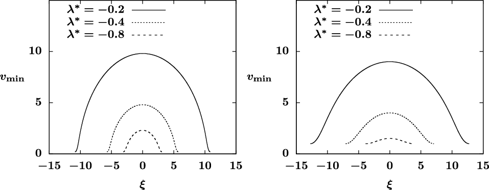When other system parameters are fixed, a larger absolute value of $\lambda^*$ , $|\lambda^*| = -\lambda^*$ , leads to an energy minimiser $v_{\min}(\xi)$ with a smaller magnitude and a smaller period (see Figure 1). The comparison between the two plots with the fibre radius $r_0 = 0.2$ and $r_0 = 1$ in Figure 1 also shows that with identical $\lambda^*$ values, a larger value of $r_0$ leads to a $v_{\min}(\xi)$ profile with a larger period and smaller spatial variations. This implies that with identical dynamic pressure, droplets on a thick fibre tend to have a smaller bead size than those on a thinner fibre.

Figure 1.

Typical profiles of the energy minimiser $v_{\min}(\xi)$ obtained by numerically solving the ODE (4.10) for $A = 0$ and $\lambda = \lambda^*$ for a range of $\lambda^*$ values with (left) $r_0 = 0.2$ and (right) $r_0 = 1$ . The minimum and maximum of the profiles are consistent with (4.17) where $C_0 = r_0 + \lambda^* r_0^2/2$ from (4.18). The periods of the solutions are given by (4.16).

Figure 2.

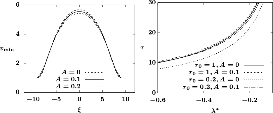
(Left) Profiles of the energy minimiser $v_{\min}(\xi)$ satisfying (4.10) for $A = 0, 0.1, 0.2$ with fixed $r_0=1$ and $\lambda=\lambda^* = -0.3$ , showing that an increasing A leads to smaller spatial variations. (Right) The period $\tau$ of energy minimisers given by (4.21) for a varying $\lambda = \lambda^*$ satisfying (4.11) with different values of A and $r_0$ . The parameter $m = 3$ is used in both figures.

Figure 2 (left) presents the effects of the stabilisation term $A/u^m$ , showing that with other system parameters fixed, a positive $A>0$ yields smaller spatial variations in $v_{\min}$ . This is also consistent with the observation drawn in [Reference Ji, Falcon, Sadeghpour, Zeng, Ju and Bertozzi10]. Similar to the $A = 0$ case, the energy minimisers $v_{\min}(\xi)$ for $A > 0$ presented in Figure 2 (left) are numerically obtained by solving the ODE (4.10) for $-\tau/2 \leqslant \xi \leqslant \tau/2$ , where the period $\tau$ is given by (4.21) and the constant $C_0$ is obtained from (4.11) with the fibre radius $r_0 = 1$ , $\lambda=\lambda^* = -0.3$ , and $m = 3$ . With different values of A and $r_0$ , Figure 2 (right) shows a comparison of the period $\tau$ of energy minimisers based on (4.21) for a varying $\lambda = \lambda^*$ that satisfies (4.11). This plot shows that when other system parameters are fixed, larger values of $r_0$ and A typically lead to a larger period $\tau$ for the energy minimiser.

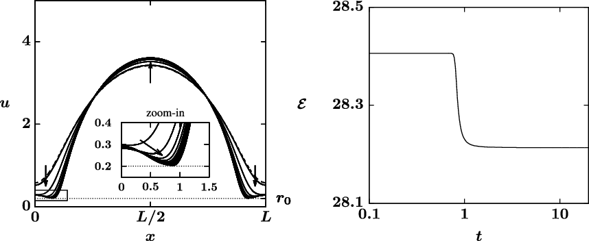
Next we explore the dynamics of the problem (2.1)–(2.3) without gravity effects, that is, without the last term $[Q(u)]_x$ . Typical dynamic simulation results of (2.1) without gravity modulation subject to periodic boundary conditions are plotted in Figure 3. The initial data for this simulation are given by $u_0(x) = v(x)$ which satisfies the ODE (4.10) with $C_0 = 0.5$ , $\lambda = -0.5$ over $0 \leqslant x \leqslant L$ for the period $L = \tau = 10.79$ obtained from (4.16). Other system parameters are $A = 0$ , $r_0 = 0.2$ , $\sigma = 0.01$ and $M = \int_0^L u^2\;dx = 68.6$ . We note that the parameter pair $(\lambda, C_0)$ do not satisfy the condition (4.11), which implies that the initial profile $u_0(x)$ is not an energy minimiser of the system. Starting from the initial profile, the dynamic solution quickly evolves into a two-hump solution with an additional local maximum at the edge $x = 0$ and $x=L$ . Moreover, a local singularity, $u = r_0$ , is approached at two global minima near $x = 0.9$ and $x = 9.9$ where the two hump solutions are connected. An inset plot is also included in Figure 3 (left) to display the dynamics near the region where the two humps are connected. The history of the energy $\mathcal{E}(t)$ in Figure 3 (right) shows that the energy is dissipating as the solution approaches to the two-hump profile. This confirms the conclusion in Theorem 2. These numerical studies are conducted using fully implicit finite differences with a uniformly spaced grid, and the numerical scheme is second-order accurate in space and first-order accurate in time. In our numerical studies, we also observed cases when a single-hump initial profile can evolve into three or more humps. We suspect that linear stability analysis for steady states of the governing PDE can lead to an estimate of the number of humps and the structure of long-time dynamics. However, a systematic investigation of this problem is beyond the scope of this paper, and we may further study this aspect of the problem in the future.

Figure 3.

Dynamics of (2.1)–(2.3) without gravity effects for $0 \leqslant t \leqslant 20$ starting from the initial data $u_0(x) = v(x)$ (dashed line) satisfying (4.10) with $C_0 = 0.5$ , $\lambda = -0.5$ . (Left) The solution profile u(x,t) and (right) the energy dissipation $\mathcal{E}(t)$ show that a two-hump solution is reached in long time. The inset plot shows the dynamics near the touch-down point where $u\approx r_0$ . Other system parameters are $A = 0$ , $r_0 = 0.2$ , $\sigma = 0.01$ .

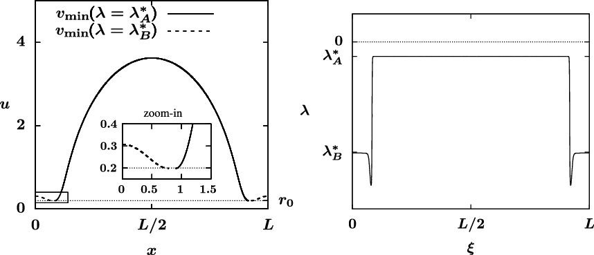
Figure 4 (right) presents the plot of $\lambda(\xi)$ corresponding to the dynamic solution in Figure 3 at time $t = 20$ . It shows that $\lambda(\xi)$ approaches a piece-wise constant function where the values of critical $\lambda^*$ are given by $\lambda^*_A = -0.523$ and $\lambda^*_B = -3.955$ , respectively. Using these critical $\lambda^*$ values, we numerically solve for the energy minimisers $v_{\min}(\xi)$ derived in Lemma 4.2 that correspond to $\lambda = \lambda^*_{A,B}$ and compare them (see Figure 4 (left)) against the long-time dynamic solution presented in Figure 3 (left). The two solutions, $v_{\min}(\lambda=\lambda^*_A)$ and $v_{\min}(\lambda=\lambda^*_B)$ , are connected at the point where the common minimum value $v = r_0$ is reached (see the inset plot in Figure 4 (left)). This comparison shows that the two-hump solution obtained from the direct numerical calculation is in good agreement with the energy minimiser characterised by $v_{\min}$ with a piece-wise constant function $\lambda(\xi) = \lambda^*_{A,B}$ .

Figure 4.

(Left) Energy minimiser $v_{\min}$ and (right) corresponding $\lambda(\xi)$ corresponding to the long-time dynamic solution u(x) at time $t = 20$ in Figure 3 (left), showing that the PDE solution presented in Figure 3 approaches to a two-hump energy minimiser characterised by a piece-wise constant function $\lambda(\xi)$ . The inset plot shows the two-hump energy minimiser near the touch-down point.

Figure 5.

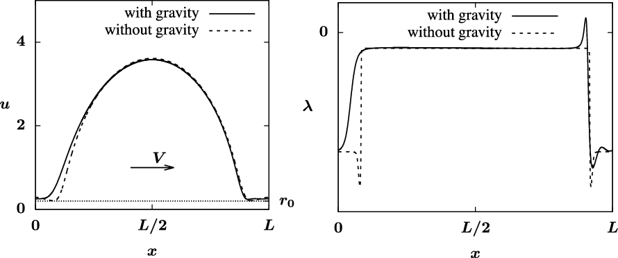
(Left) Solution profiles u(x) and (right) the corresponding $\lambda(x)$ profiles of a travelling wave solution satisfying (1.4) with gravity effects at a speed $V = 5.12$ compared with long-time dynamic solution shown in Figure 3 without gravity effects. System parameters are identical to those used in Figure 3.

The gravity effects incorporated in (2.1)–(2.3) can lead to a travelling wave solution at a speed V characterised in the travelling wave PDE (4.1). To better understand the influence of gravity effects in the model, we numerically solve the equation (2.1) starting from the two-hump profile obtained from the simulation shown in Figure 3 where gravity effects are excluded. The system parameters are also set to be identical to those used in Figure 3. The simulation shows that the dynamic solution quickly converges to a travelling wave at a constant speed $V = 5.12$ . A comparison of this travelling wave solution and the two-hump profile without gravity is shown in Figure 5 (left), where the spatial symmetry around $x = L/2$ in the travelling wave solution is broken due to the presence of gravitational effects. Figure 5 (right) depicts the corresponding $\lambda$ profiles for the two solutions. This plot reveals that without gravity the $\lambda$ profile for the two-hump solution approaches a piece-wise constant function, while the travelling wave solution only keeps the large hump corresponding to $\lambda=\lambda_A^*$ and the small hump with $\lambda=\lambda_B^*$ is saturated by the gravity. In addition, the global minimum of the travelling wave solution is above the fibre radius parameter $r_0 = 0.2$ , which indicates that the gravitational effects prevent the singularity observed in the no-gravity case from happening.

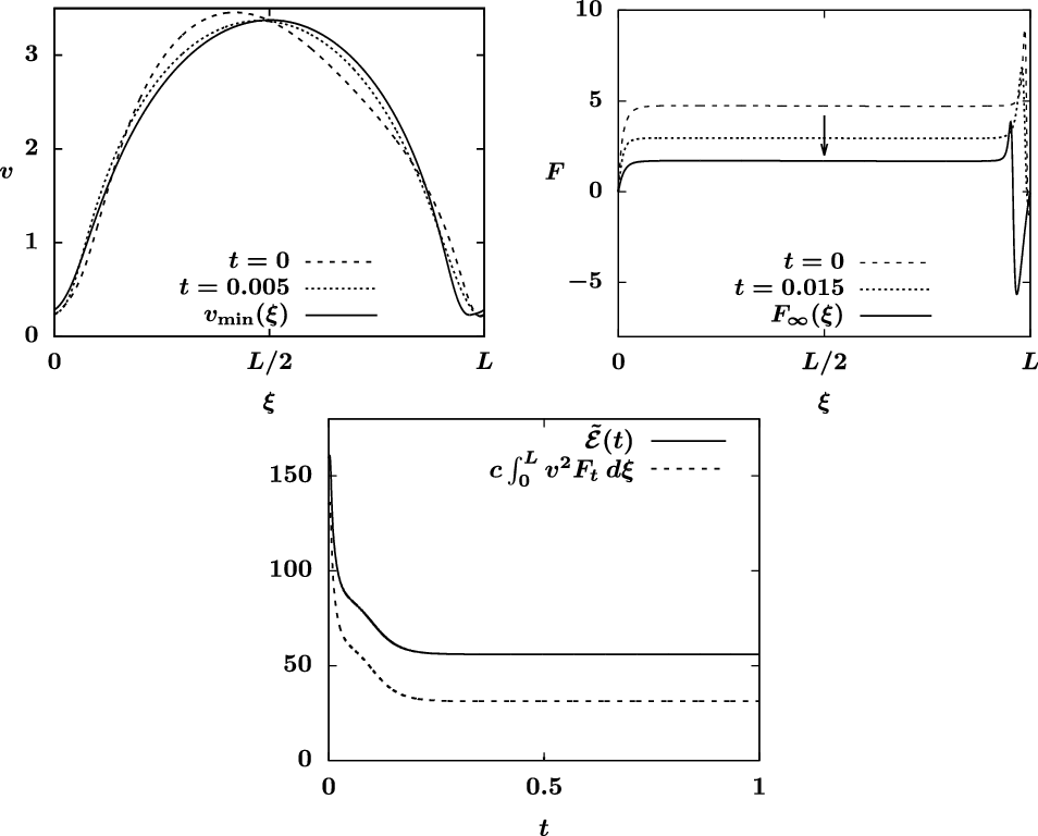
Finally, we investigate the convergence to travelling wave solutions with the presence of gravity using the PDE (4.1) in the moving reference frame with $\mu = 1$ . A travelling wave solution $v_{\min}(\xi)$ at a propagating speed V is a steady state of PDE (4.1) and satisfies the fourth-order ODE (5.1) for $v(\xi)$ on a periodic domain $0 \leqslant \xi \leqslant L$ ,

(5.1) \begin{equation}\sigma^{-1} [ Q(v) \bigl( (\Phi'(v_{\xi}))_{\xi} - v^{-1} f(v_{\xi}) + A v^{-m} \bigr)_{\xi} ]_{\xi}+ (Q(v) - \tfrac{V}{2} v^2)_{\xi} = 0.\end{equation}

The profile of the travelling wave is determined by the period L and the mass $M = \int_0^L v^2\;d\xi$ . For a given (L, M) pair, we numerically solve the travelling wave ODE (5.1) for $v_{\min}(\xi)$ and the speed V simultaneously on a periodic domain $0\leqslant \xi \leqslant L$ using finite differences. A continuous family of travelling wave solutions to (5.1) parametrised by (L, M) can be identified. Using a branch continuation method, we numerically track the travelling waves as the parameter L or M changes. Similar parametric and pseudo-arclength continuation methods are commonly used for bifurcation analysis [Reference Ji and Li11,Reference Ji and Witelski14,Reference Keller16]. For $L = 9$ and $M = 57.2$ , we obtain a travelling wave solution $v_{\min}(\xi)$ with the associated velocity $V = 4.24$ (see the solid curve in Figure 6 (top left)). This velocity agrees with the analytical expression for V provided in Lemma 4.4. The other system parameters are identical to those used in Figure 3.

Figure 6.

PDE simulation of (4.1) with $\mu = 1$ starting from the initial data $v_0(\xi)$ in (5.2) with $\bar{f}=1$ , showing (top left) the convergence of the PDE solution $v(\xi,t)$ to the travelling wave $v_{\min}(\xi)$ , (top right) the corresponding evolution of $F(\xi,t)$ and (bottom) the decay of modified energy $\tilde{\mathcal{E}}$ and $\int_0^L v^2 F_t d\xi$ in time. The travelling wave $v_{\min}(\xi)$ satisfies the ODE (5.1) and is associated with $L = 9$ and $M = 57.2$ . A scaling constant $c = 5\times 10^{-5}$ is used to display both curves $\tilde{\mathcal{E}}$ and $\int_0^L v^2 F_t d\xi$ in a comparable range. Other system parameters are identical to those used in Figure 3.

Starting from a perturbed initial condition

(5.2) \begin{equation} v_0(\xi) = v_{\min}(\xi)+\bar{\epsilon}\sin(2\pi \bar{f}\xi/L),\end{equation}

where $\bar{\epsilon}$ is the magnitude and $\bar{f}/L$ is the frequency of the perturbation, we numerically solve the travelling wave PDE (4.1) and observe that the PDE solution converges to the travelling wave $v_{\min}(\xi)$ as $t\to \infty$ . Here we select the magnitude of the perturbation

(5.3) \begin{equation} \bar{\epsilon} = -\frac{4}{L}\int_0^Lv_{\min}(\xi)\sin(2\pi \bar{f}\xi/L)\;d\xi, \end{equation}

such that the initial data satisfy the condition $\int_0^L v_0^{2}\;d\xi = \int_0^L v^2_{\min}\;d\xi = M$ which is necessary for the convergence to the travelling wave $v_{\min}$ due to the conservation of mass condition. For the simulation shown in Figure 6, we set $\bar{f} = 1$ which corresponds to the magnitude $\bar{\epsilon} = 0.51$ based on the formula (5.3) for $L = 9$ . To calculate the modified energy $\tilde{\mathcal{E}}(t)$ defined in (4.31), we specify $\nu(t)$ in the definition of $F(\xi,t)$ in (4.30) based on the formula

(5.4) \begin{equation} \nu = \frac{\frac{V}{2}\int_0^L \frac{v^2(\xi,t)}{Q(v(\xi, t))}\;d\xi -L}{\int_0^L\frac{1}{Q(v(\xi, t))}\;d\xi}\end{equation}

so that condition (4.32) is satisfied. Figure 6 (top right) depicts the evolution of $F(\xi,t)$ in time as the PDE solution converges to the travelling wave, showing that the condition $F(0,t) = F(L,t) = 0$ in (4.34) is satisfied. The plot in Figure 6 (bottom) shows that as the travelling wave $v_{\min}(\xi)$ is approached, both the modified energy $\tilde{\mathcal{E}}(t)$ and the corresponding $\int_0^L v^2 F_t\;d\xi$ decay in time, which is consistent with the result shown in Lemma 4.3. We note that while the simulations in Figures 4 and 6 are conducted with $A = 0$ , similar dynamics are observed for simulations with small stabilisation parameter $A > 0$ .