Introduction

The study of ice crystals has proven important for understanding and modelling the flow of ice. Many conventional flow models for large ice sheets work under the assumption that ice is isotropic, but, in fact, many properties of ice crystals in ice sheets are generally not isotropic (Reference Budd and JackaBudd and Jacka, 1989; Reference AlleyAlley, 1992). In order to develop improved flow models we need to obtain a better understanding of how the crystals behave in the ice sheets. How do ice crystals grow, deform, split, reorient and interact as they flow in the ice sheets? the temperature and stress histories of the ice, as well as the content of impurities in the ice, are among the deciding factors, but the complex relationships are not well understood. With the recent developments in digital technology we have the possibility for improving our experimental knowledge of ice-crystal properties.

Traditionally the study of ice-crystal textures and fabrics has been carried out manually by use of a Rigsby Universal Stage (Reference LangwayLangway, 1958). A thin section of an ice sample is placed horizontally on a stage between two crossed linear polarizers with a light source placed below the lower polarizer. Because of the double refractivity of ice and due to the different orientation of the crystals in the sample, the crystals will appear with different colours when observed through the upper polarizer. the c-axis orientation of a crystal is determined by rotating the sample stage in three dimensions after a specific procedure to obtain a position where the crystal appears black and the direction of the c axis is known. Crystal sizes can be determined, for example, by the linear intercept method, where the number of crystals crossing a line across the sample is counted, or by the mean area method, where the number of crystals in a given area is counted.

Recently the development of the digital camera and advanced imaging software has allowed for automation of ice-crystal studies. Instruments for automatic measurements of c-axis orientation of ice crystals have been developed in Japan (Wang and Azuma, 1999), in Australia (personal communication from D. Russell-Head, 2001) and in the United States (Reference WilenWilen, 2000). the automatic instruments have the advantage of being able to measure the properties of many crystals rapidly, and they therefore strongly improve the statistics of measurements.

In this study we present a detailed study of crystal properties of ice from the mild climatic period interstadial 3 (IS3) that occurred in Greenland during the last glacial period about 25 kyr BP. the samples are taken from the Greenland Icecore Project (GRIP) ice core which was drilled at the summit of the Greenland ice sheet during the summers of 1989– 92 (Reference DansgaardDansgaard and others, 1993; GRIP Project Members, 1993). IS3 lasted for about 300 years and is likely to have been up to 13˚C warmer than the ambient cold glacial period (Reference Johnsen, Dahl-Jensen, Dansgaard and GundestrupJohnsen and others, 1995).

The purpose of the present study is partly to explore the new automatic methods for studying ice-crystal properties, and partly to study a possible variability in crystal properties across a Greenland glacial interstadial. IS3 is chosen because it is one of the best-studied sections of the GRIP ice core for which profiles of chemical impurities and dust have been measured.

Reference Thorsteinsson, Kipfstuhl and MillerThorsteinsson and others (1997) measured the profiles of crystal size and c-axis orientation along the GRIP ice core by manual methods, and in the nearby Greenland Ice Sheet Project 2 (GISP2) ice core these properties were studied by Reference GowGow and others (1997). from these and previous studies we know that crystals in the cold Greenland glacial period are the smallest in the Greenland ice sheet, with most of them having cross-sectional areas of <10mm². the extremely small crystal size is thought to be related to the high concentration of soluble and/or insoluble impurities in the glacial ice (Reference Alley, Perepezko and BentleyAlley and others, 1986; Reference Langway, Shoji and AzumaLangway and others, 1988). It is currently debated which impurities have most influence on the crystal size. Due to the dominant uniaxial compression of the ice at the GRIP drill location, the orientation of c axes in the glacial ice is dominantly vertical. the general trend during the glacial is an increasing degree of orientation of c axes towards vertical with depth/age. However, detailed investigation suggests that the c-axis orientations may also be influenced by impurity content of the ice.

Methods

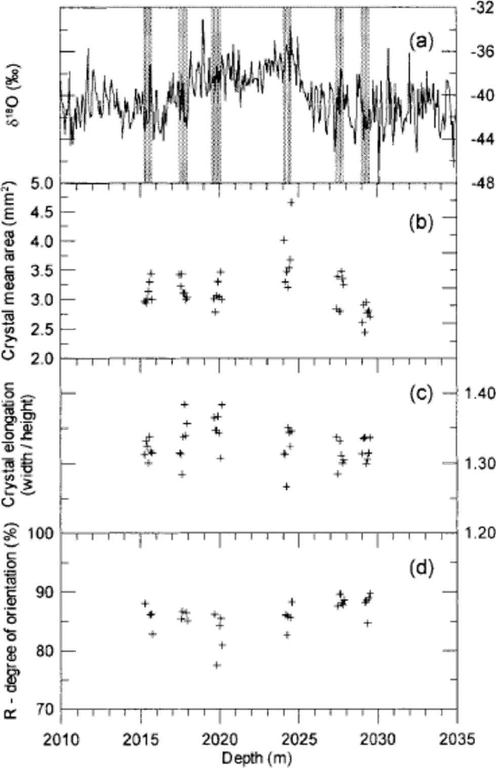
Ice samples were prepared in a cold room at the Copenhagen ice-core laboratory, where the GRIP ice core is stored at –25˚C. Six vertical sections of 55 68 ×1cm³ were cut along the GRIP core around the IS3 event. the sections were taken in pairs of two from before, during and after IS3, with IS3 defined by the δ¹⁸O profile to be the depth interval 2018– 2026 m.The sampling depths are shown in Figure 1a and given in Table 1. With this sampling we do not obtain a continuous profile across IS3, but the sampled sequences are sufficiently long to average out the annual cycle, and they enable comparison with δ¹⁸O, dust and chemistry profiles. Each section was split into seven samples each 7–8 cm long to obtain a total of 42 samples. the ice surface was smoothed with a microtome knife, and the samples were mounted on glass plates by freezing water droplets along the sides. These ``thick’’ sections were photographed for visual core-stratigraphy determination. the samples were then sliced down to 0.5 mm thin sections in a microtome bench. Generally the sample quality was good, but a few samples had severe cracks and could not be used.

Fig. 1

(a) the GRIP δ¹⁸O profile across the glacial IS3 with indication of the six 55 cm long sampling sections (grey bars). Each section is divided into seven samples each 7–8 cm long. (b–d) Crystal mean area (b), mean crystal elongation (c) and degree of orientation (d) of the samples.

Table 1.

The six sampled depth intervals with indication of the mean δ¹⁸O value of the sampled ice and the obtained area-distribution parameters

Digital pictures for crystal-boundary determination were obtained with a simple set-up. A thin section was mounted horizontally in the Rigsby Stage and photographed with a standard digital camera at a resolution of about 17 pixels mm^–1. Because not all crystal boundaries will be visible in a single image, four images were obtained at four different sample orientations. for each picture the linear polarizers were rotated 5–10˚ in the horizontal plane, while the sample and camera were kept fixed. It was found that the crystals show the greatest variability in colour and intensity when the dominant c-axis orientation of the sample is parallel to the direction of the linear polarizer, and the pictures were obtained in the angular neighbourhood of this direction. Because the samples are vertical sections, the crystals are relatively easy to distinguish and we found that four images were sufficient to identify almost all the crystal boundaries.

The crystal boundaries were determined from the digital pictures using the imaging software package Image-Pro.Most of the boundaries were determined automatically by a macro following the procedure outlined by Reference Gay and WeissGay and Weiss (1999) and Wang and Azuma (1999). Briefly, the images are separated into the colour channels R, G and B, and a filter is applied which determines the crystal boundaries from intensity contrasts in the image. This procedure is applied to each of the four images to obtain four independently determined boundary outlines. These are stacked digitally to obtain an outline that contains almost all the boundaries in the sample. After the automatic treatment, the outlines were edited manually to correct for crystal boundaries that were obviously wrong or not determined. the method is described in detail in Reference HansenHansen (2001).

The c-axis orientations of crystals in selected samples were measured on the Automatic Ice Fabric Analyzer (AIFA) at the Alfred Wegener Institute (AWI) in Bremerhaven, Germany, following the procedures described by Wang and Azuma (1999). AIFA works with digital images of the samples with a resolution of about 8 pixels mm^–1, which is a somewhat low resolution for determining the c-axis orientation of the smaller crystals in the samples. the crystals to be measured were selected manually. In order to verify the measurements of the critically small crystals, most c-axis orientations were measured twice.

Samples for measurements of concentrations of insoluble dust and of chemical impurities across IS3 were obtained in 5 cm resolution at GRIP, and the measurements were carried out at the University of Copenhagen. Dust concentrations were determined on a Coulter counter as described in Reference SteffensenSteffensen (1997), and the concentrations of Ca²⁺, SO₄ ^2–, Cl^– and NO₃ ^– were measured by ion chromatography following the methods outlined in Reference Steffensen, Clausen, Hammer, Legrand and deAngelisSteffensen and others (1997).

Results

The procedure to determine the crystal boundaries worked generally well. Roughly 10% of the boundaries were edited or added manually after the automatic processing. After this treatment we are confident of having identified all the crystal boundaries in the samples within 5%. In the end, it is a question of definition whether two neighbouring crystals with almost the same orientation are two separate crystals or just one slightly bent crystal. We determined about 1500 crystals in each thin section, and in total more than 60 000 crystals were identified. An example of a crystal outline is shown in Figure 2. When the crystal outlines are determined, the imaging software provides a suite of parameters for the individual crystals (e.g. the coordinates of the centre of mass, the area and the dimensions). the crystal area provided by the software does not include the crystal boundary. This gives rise to an area defect, as the sum of areas of crystals is about 10% smaller than the sample area. We made a weighted renormalization of the areas to correct for this. Figure 1b shows the mean crystal area of each thin section on a depth scale. We notice that crystals from the beginning of IS3 (2024m depth) are larger than average, whereas crystals in the oldest sample (2029m depth) are smaller than average. Three crystal area distributions are presented in Figure 3a: one distribution for the entire crystal population of the samples, one distribution for the crystals within IS3, and one distribution for the crystals before and after IS3. In a semi-log plot the area distributions show a distinct bell-shaped form, and they can be fitted rather well with lognormal distributions of the form

Fig. 2

An example of a vertical 1.0 cm thick section (top) with clearly visible cloudy bands, and the corresponding 0.5 mm thin section (bottom) viewed between crossed polarizers. the ice-core direction is horizontal, with increasing age to the right. the sample size is ~768 cm²and the sample contains about 1500 crystals. the automatically identified crystal boundaries are indicated with thin white lines. the cloudy band on the left side of the sample is clearly seen as a band of small crystals in the thin section, while the broader cloudy band on the right appears less well defined in the thin section.

Fig. 3

Crystal area distributions and fit functions. (a) the total distribution of all measured crystals (solid dots) of the crystals within IS3 (open circles), and of those before and after IS3 (open triangles). Each distribution is fitted with a single lognormal distribution. (b) the distribution of all measured crystals (solid dots), with a fit function (thick curve) composed of two lognormal distributions (thin curves). (c) the distribution of crystals within selected cloudy bands (open circles), of crystals outside cloudy bands (open triangles), and of the sum of the two distributions (solid dots). Each distribution is fitted with a lognormal distribution.

where N is the total number of crystals, N₀ is the amplitude of the distribution, μ is the mode or the lognormal mean, and σ is the lognormal standard deviation. Fitted lognormal distributions are shown in Figure 3a, and in Table 1 the lognormal parameters are given together with the mean crystal areas of the six sampled depth intervals. the average crystal area within the climatically mild IS3 is 3.36 mm², while the crystals before and after IS3 have an average area of 3.04 mm². the mean areas agree well with the GRIP crystal sizes measured by Reference Thorsteinsson, Kipfstuhl and MillerThorsteinsson and others (1997), although those authors measured crystal sizes by the linear intercept method, so the results are not directly comparable. the crystals are somewhat elongated horizontally due the vertical strain of the ice. We calculated the mean crystal elongation of each thin section, and the result is shown in Figure 1c. Crystal dimensions in a few horizontal thin sections were determined in order to verify the symmetry of crystal dimensions with respect to the core axis. Again the results are in good agreement with those of Reference Thorsteinsson, Kipfstuhl and MillerThorsteinsson and others (1997).

The c-axis orientations were determined in 16 thin sections, and about 500 crystals were measured in each thin section. Most c-axis orientations were determined twice at different locations in the crystal. Based on those double measurements, we had to discard up to 10% of the measurements in a thin section, as the measurements did not reproduce. the reason for this is that the smaller crystals are not well resolved with the present configuration of AIFA. Higher resolution of the images could probably help to solve the problem. After discarding the wrong measurements we have good confidence in the results.

The c-axis orientations determined in the vertical samples were rotated to obtain a top-view equal-area Schmidt projection following standard procedures. As expected at this depth, the fabric is strongly vertical in all samples (Reference Thorsteinsson, Kipfstuhl and MillerThorsteinsson and others, 1997). Typical Schmidt diagrams are shown in Figure 4. for each measured thin section we calculate the degree of orientation R, which is defined as

Fig. 4

Top-view Schmidt diagrams of typical samples. the samples are from within IS3 (a) and after IS3 (b), and from within selected cloudy bands (c) and outside those bands (d). Each diagram contains 200 randomly selected c axes. the R parameter of the four diagrams is 86%, 88%, 85% and 91%.

where N is the number of crystals and S is the length of the vector sum of the normalized c axes (Reference Thorsteinsson, Kipfstuhl and MillerThorsteinsson and others, 1997). R is a measure of how well the c axes are aligned. If the c axes are randomly distributed we have R = 0%, while R = 100% if all c axes are pointing in the same direction. the R values obtained are shown in Figure 1d. They are seen to agree well with the value of approximately 85% determined byReference Thorsteinsson, Kipfstuhl and MillerThorsteinsson and others (1997) for samples taken from nearby depth intervals in the GRIP core. Due to the low inter-sample variability in the degree of orientation, other commonly used orientation parameters, such as the spherical aperture, or the eigenvalues of the orientation tensor, do not provide additional information and they are not shown.

Discussion

The crystal area distribution

As seen in Figure 3a the cross-sectional area distribution of the crystals can be well fitted with a single lognormal distribution. However, the fit is strongly improved if the shoulder on the left side of the distribution is fitted with a second lognormal distribution, as in Figure 3b. This shoulder is also present in the distributions shown in Figure 3a and c, but for clarity only the major fit is shown here. Although lognormal distributions have been observed in the context of computer simulations of normal crystal growth of metals (Reference Anderson, G. S. and SrolovitzAnderson and others, 1989), it isbeyond the scope of this paper to discuss the theoretical background for this area distribution in the context of ice. for the moment, we will simply assume that the area distribution is a lognormal distribution, and we will discuss potential sources for the small lognormal distribution in Figure 3b, which is centred around 0.5 mm².

Our first suggestion is that this distribution could be attributed to crystals in cloudy bands, which are smaller than the average crystals in the ice (see Fig. 2). We therefore selected seven thin sections where cloudy bands are clearly visible, and plotted the area distributions of crystals from within and outside the cloudy bands. the result is shown in Figure 3c and is discussed further in a following section. the difference between the two groups of crystals is clear: crystals within the cloudy bands are significantly smaller than those outside the bands. However, the crystals within the cloudy bands are much larger than those in the small distribution in Figure 3b.

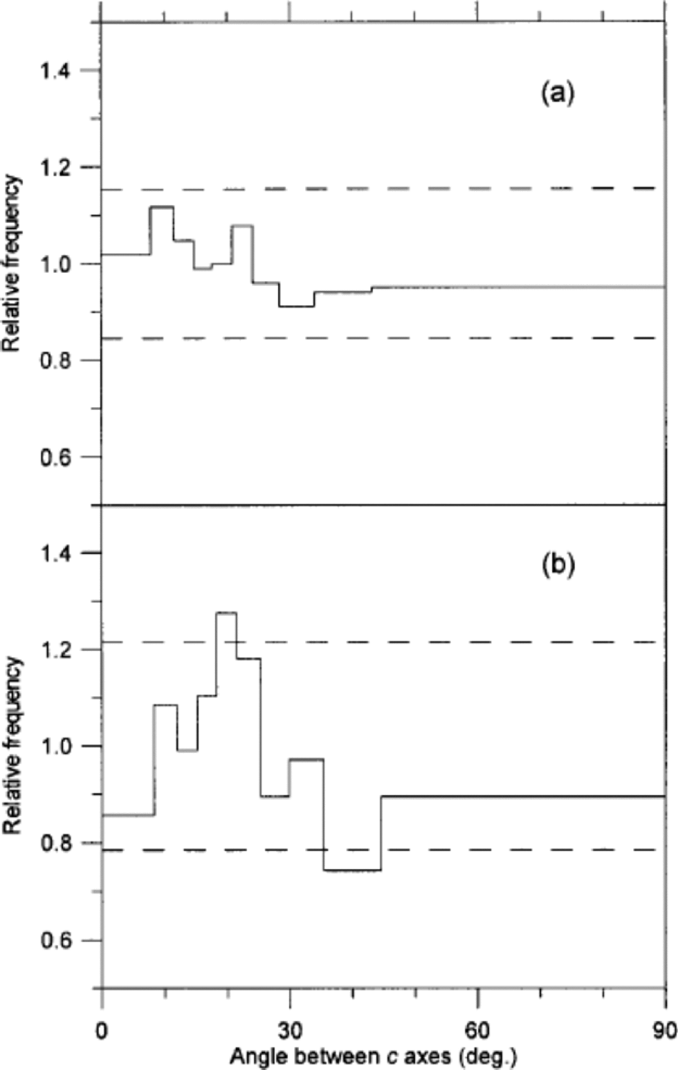
Our second suggestion for this distribution is that its source could be related to crystal polygonization. Some polygonization is evidenced in the samples by strain shadows in large crystals. If we imagine that small crystals continuously disintegrate from larger crystals because of ice deformation, we could end up with a population of small crystals. to investigate this idea we studied the angles between c axes of adjacent crystals in two thin sections. If polygonization is significant we would expect to find a high fraction of ``recently’’ separated adjacent crystals with almost parallel c axes (Reference Alley, Gow and MeeseAlley and others, 1995). In order to cover both cold and mild climate, the two sections were selected to be an interstadial sample with small crystals and the stadial sample with the largest crystals. the result of the analysis, which is presented in Figure 5, shows that polygonization can be a dominant mechanism neither in the cold nor in the milder period, although it could actually contribute to the small crystals seen in the area distributions in Figure 3.

Fig. 5

Distribution of angles between c axes of adjacent crystals in a sample from after IS3 (a) and in a sample from IS3 (b). the figure follows the notation of Reference Alley, Gow and MeeseAlley and others (1995): A distribution of the angles between c axes of 10 000 randomly selected pairs of crystals in the sample is obtained. the width of each bin is defined to contain 10% of this distribution. Then the angles between all neighbouring pairs of crystals are obtained. the amplitude of each bin is now given as the ratio of the two distributions (e.g. in (b) 10% of the angles between the randomly selected pairs of crystals fall in the angular range 0–8˚, while 0.86×10% = 8.6% of the angles between neighbouring crystals fall into the same range). the dashed lines mark the level of significant deviation from a random distribution at 95% confidence level. (a) is obtained from 542 crystals and 1021 pairs of neighbours, and (b) is obtained from 331 crystals and 525 pairs of neighbours.

Our last suggestion for small crystals is related to the form of the crystals in three dimensions. It should be kept in mind that the area distribution we are presenting is a cross-sectional projection of three-dimensional crystals, which are not necessarily intersected at their maximum area. If the three-dimensional crystals have a rugged surface (e.g. non-convex form with many ``corners’’) this could give rise to a high ratio of ``small’’crystals in a cross-sectional thin section. Indeed the shape of the crystals in the thin sections is not very regular, but in order to test this rather speculative idea we would need to carry out a crystal study in three dimensions.

Crystal growth

The glacial IS3 appears to be a suitable climatic event for studying variability in crystal sizes. the temperature of the snow deposited during the event was higher than that of snow deposited before and after the event. However, because the event is so relatively short (300 years), the temperature difference in the ice will have equalized by heat diffusion during a period that is short compared to the age of the ice (25 kyr). Therefore, except for a limited period after deposition, both the temperature and the stress histories are almost the same for ice within and adjacent to IS3. Those quantities are therefore not likely to be the dominant factors in explaining the variability in crystal size across IS3. Other candidates are the impurities in the ice. Several of the major impurities found in ice cores have been suggested as the controlling factor for crystal growth (Reference Alley, Perepezko and BentleyAlley and others, 1986; Reference Langway, Shoji and AzumaLangway and others, 1988). One problem in determining which impurity(ies) may be the most important for crystal growth is that many of them are varying in phase in the ice.

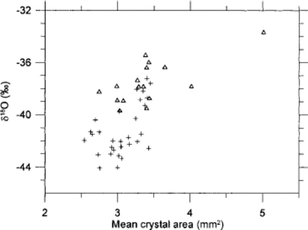
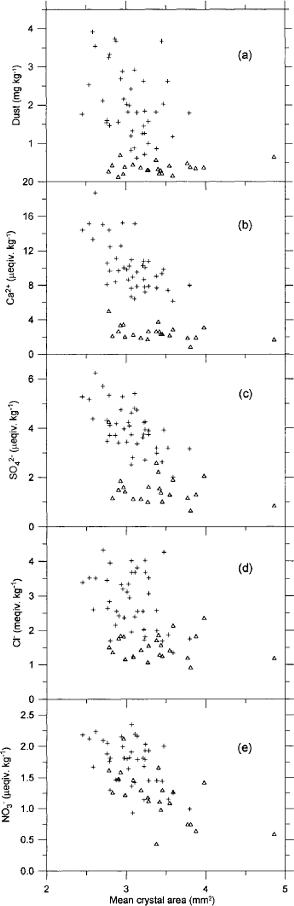
In Figure 6 the crystal areas are seen to correlate to some degree with δ¹⁸O, although the scatter of points is quite distinct. the trend is towards smaller crystals in the coldest periods and larger crystals for less cold climate. Figure 7 shows the mean crystal area vs the concentrations of insoluble dust, Ca²⁺, SO₄ ^2–, Cl^– and NO₃ ^– in the ice. As seen in Figure 7a, the dust concentration does not correlate with the ice-crystal areas at all. of the chemical impurities, Ca²⁺ correlates least with crystal area, having the crystals from within and outside IS3 separating into two distinct groups. for SO₄ ^2– the correlation is quite good for stadial samples, but the interstadial samples do not show a significant correlation. for Cl^– the interstadial samples almost anticorrelate with the crystal area. In contrast, NO₃ ^– shows quite good correlation with both stadial and interstadial samples, and the two groups of samples mix quite well in the plot. from this we conclude that, if the variability in crystal areas is due to the impurity content of the ice, NO₃ ^– is most likely to be the determining factor. This result is somewhat surprising since the NO₃ ^– concentration is relatively low compared to the other ion concentrations. the crystal areas have also been compared to the concentrations of Na⁺, Mg²⁺ and K⁺ (Reference HansenHansen, 2001), but as those quantities correlate with the ions shown in Figure 7 the comparisons do not provide much additional information, and the results are not shown. Mg²⁺ and K ⁺ vary quite closely with Ca²⁺, whereas Na⁺ correlates well with Cl^–. the NH₄ ⁺ concentration in the ice is very low−often below detection level−and could not be used for comparison.

Fig. 6

Correlation of mean crystal area with δ¹⁸O in 7 cm resolution. Samples from within IS3 are shown as open triangles, and samples from before and after IS3 are shown as crosses.

Fig. 7

Correlation of mean crystal area with insoluble dust (a) and with the soluble impurities Ca²⁺(b), SO₄ ^2–(c), Cl^–(d) and NO₃ ^–(e). the resolution is 5 cm. Samples from within IS3 are shown as open triangles, and samples from before and after IS3 are shown as crosses.

Cloudy bands

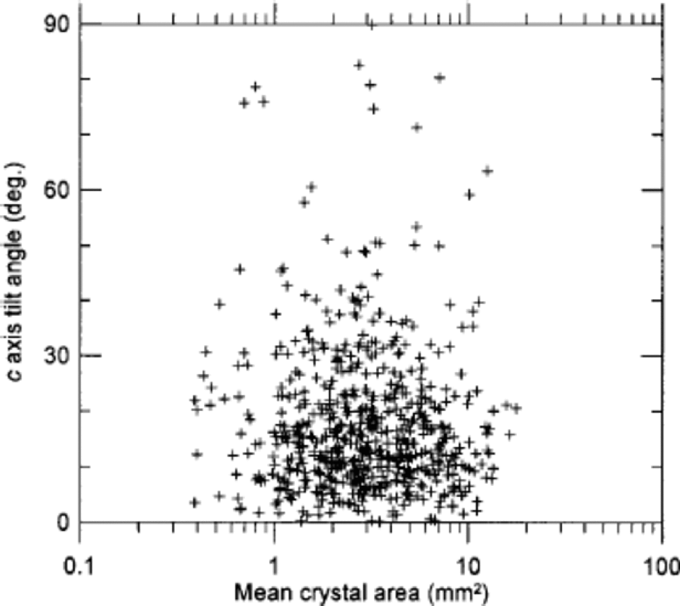
We made a small investigation of texture and fabrics in cloudy bands, which are very prominent in the cold stadial ice (see Fig. 2). from visual selection of cloudy bands in seven thin sections, we separated the crystals within the bands from those in the surrounding clear ice. A total of 11000 crystals were included in the exercise. the area distributions of the two groups are shown in Figure 3c. the crystals outside the cloudy bands are roughly twice as large as those within the bands, and the lognormal fit of the cloudy-band crystals is slightly narrower than that of the average sample (Table 1). As pointed out by Reference MiyamotoMiyamoto and others (1999), the fabrics in the GRIP cloudy bands are less well collimated than the fabrics of the clear ice. on average, we obtain R = 83% within the bands and R = 88% outside. This seems a relatively strong effect compared to the rather conservative behaviour of the R parameter (Fig. 1d). This correlation between fabrics and texture is not generally true in the ice. In Figure 8 the area distribution vs the direction of c axes in a thin section is shown without any pronounced cloudy bands. In this example no correlation between texture and fabric is seen. So the cloudy bands probably constitute a special case, which may have implications for the flow of cold glacial ice.

Fig. 8

The crystal area vs the tilt angle of the c axis of 600 crystals in a sample from within IS3 that does not contain any clearly visible cloudy bands. the tilt angle is the angular deviation of the direction of the c axis from vertical.

Conclusions

A semi-automatic method for identifying the crystal boundaries in thin sections of ice worked satisfactorily. the area distribution of the entire crystal population, as well as subsets of this, is fitted very well by a lognormal distribution function, and the standard deviation of the various distributions is almost constant. We do not provide a theoretical model for this distribution.

Crystals from within IS3 are on average somewhat larger than crystals outside IS3, but the difference is only a small fraction of the mean. of the various impurities measured across the IS3 ice, we find NO₃ ^– correlates best with the average crystal areas. This suggests NO₃ ^– as a controlling factor for crystal sizes in Greenland glacial ice. Insoluble dust, Ca²⁺, SO₄ ^2– and Cl^– seem less important in this context.

The fabrics around IS3 follow the expected pattern of a vertical single maximum. In clearly visible cloudy bands, the c axes are slightly less well collimated than in the surrounding clear ice. This, combined with the significantly smaller crystals in the cloudy bands, makes us speculate that the cloudy bands contain high concentrations of impurities, which influence both the textures and fabrics of the ice. the hypothesis can be tested when measurements of impurity concentrations become available at a resolution comparable to the scale of the cloudy bands.