1 Introduction
Capturing word meaning is one of the challenges of natural language processing (NLP). Taxonomies and, in general, semantic networks of words (Miller Reference Miller1995) are often used as formal models of meaning in intermediate NLP tasks, such as word sense disambiguation (Agirre and Rigau Reference Agirre and Rigau1996), selectional preference induction (Resnik Reference Resnik1993), and textual entailment recognition (corley and Mihalcea Reference Corley and Mihalcea2005; Zanzotto et al. Reference Zanzotto, Pennacchiotti and Moschitti2009), as well as in final applications, such as question-answering (Clark, Fellbaum and Hobbs Reference Clark, Fellbaum and Hobbs2008). In these networks, words are connected with other words by means of taxonomic and, in general, semantic relations. This is a way to capture part of the knowledge described in traditional dictionaries. For example, this informal definition of ‘wheel’:
a wheel is a circular frame turning about an axis . . . used for supporting vehicles. . .
contains a taxonomic relation, i.e. the wheel is a circular frame, and a sort of part-of relation, i.e. the wheel is used for supporting vehicles.
Yet, to be effectively used in applications, semantic networks have to be large or, at least, adapted to specific domains. Even large lexical knowledge repositories (e.g. WordNet, Miller Reference Miller1995) are extremely poor when used in specific domains, such as medicine (Toumouth et al. Reference Toumouth, Lehireche, Widdows and Malki2006). Automatically creating, adapting, or extending existing knowledge repositories using domain texts is, then, a very important and active area. Building on the distributional hypothesis (Harris Reference Harris, Katz and Fodor1964) or on the notion of the lexico-syntactic patterns (originally used in Robison Reference Robison1970), a large variety of methods have been proposed: ontology learning methods (Medche Reference Medche2002; Navigli and Velardi Reference Navigli and Velardi2004; Cimiano, Hotho and Staab Reference Cimiano, Hotho and Staab2005) in knowledge representation as well as knowledge harvesting methods in NLP (Hearst Reference Hearst1992; Pantel and Pennacchiotti Reference Pantel and Pennacchiotti2006). This learning task is generally seen as a classification (Pekar and Staab Reference Pekar and Staab2002; Snow, Jurafsky and Ng Reference Snow, Jurafsky and Ng2006) or a clustering (Cimiano et al. Reference Cimiano, Hotho and Staab2005) problem.
Many models for learning generic semantic relations between words are binary classifiers (Pantel and Pennacchiotti Reference Pantel and Pennacchiotti2006; Snow et al. Reference Snow, Jurafsky and Ng2006). In this case the task is deciding whether the two words are in a specific semantic relationship. Lexico-syntactic patterns are used as features to build vector spaces for word pairs where binary classifiers are applied. Feature values describe the correlation between contexts of word pairs and specific patterns. These approaches are extremely relevant, as the task is seen as a simple binary classification problem and not as a more complex multi-classification task (Pekar and Staab Reference Pekar and Staab2002).
The above learning models have two major limitations. The first limitation is that these models do not explicitly exploit transitivity when learning taxonomies or networks of words. Transitivity, when relevant, is not used to better induce confidence values for extracted semantic relations. Even where transitivity is explicitly used (Snow et al. Reference Snow, Jurafsky and Ng2006), it is not directly exploited to model confidence values but is used in an iterative process to maximize the likelihood of the entire semantic network. The second limitation is instead more general. Given the nature of the knowledge learning problem, machine learning algorithms are exposed to vector spaces that can be huge. As relevant patterns are not known in advance, all possible patterns are taken as features to detect a particular relation among words. Large feature spaces can have negative effects on machine learning models, such as increasing the computational load and introducing redundant or noisy features. These problems can be solved using feature selection (Guyon and Elisseeff Reference Guyon and Elisseeff2003). Yet, supervised models cannot be easily applied. When expanding existing taxonomies, we generally have only positive examples as training. Negative cases are only artificial. We then need to apply unsupervised feature selection models.
In this paper, we address the above two issues transforming the limitations into opportunities. We propose a novel probabilistic method for learning taxonomies that (1) explicitly models transitivity for deriving confidence weights; and (2) naturally exploits vector space-reduction techniques for selecting features within the estimation of the probabilistic model. To exploit transitivity of semantic relations, we define two probabilistic models: the direct probabilistic model and the induced probabilistic model. The first is directly estimated on observations over text collections. The second exploits transitivity and the direct probabilistic model to induce probabilities of derived events. As unsupervised model for selecting features, we propose to use singular value decomposition (SVD) in an innovative way to estimate direct probabilities. In a nutshell, leveraging on the particular direct probability estimation model, we use SVD as a computationally simpler and more accurate way to compute the pseudo-inverse matrix needed in logistic regression.
The rest of the paper is organized as follows. After the related work (Section 2), we firstly give a general idea of our induced probabilistic model and define the probabilistic definition of a concept (Section 3). Then, we formally present our model (Section 4) and describe a way to use SVD as unsupervised feature selection model for estimating direct probabilities (Section 5). To describe this latter idea, we need to fully describe our direct probabilistic taxonomy learning model and the way of computing the logistic regression. In Section 6, we introduce the iterative probabilistic model, i.e. an existing probabilistic taxonomy model (Snow et al. Reference Snow, Jurafsky and Ng2006). We empirically show that our induced probabilistic taxonomy learning model outperforms the existing iterative probabilistic model and that our unsupervised feature selection method has positive effect on the performance (Section 7). Finally, we draw some conclusions and plan the future work (Section 8).
2 Related work
Effective methods for learning knowledge bases from texts can give an important boost to knowledge-based systems, i.e. systems using declarative knowledge to perform some tasks. The need of such learning methods has generated a large variety of models. In this section we first analyze some of these models in order to motivate our choice of working within a probabilistic framework for leveraging transitivity in learning taxonomies or semantic networks. Then we quickly describe supervised and unsupervised models for feature selection and how they have been applied to taxonomy learning models.
2.1 Taxonomy learning models
Models for automatically learning semantic networks of words, such as taxonomies, from texts use variants of the distributional hypothesis (DH) (Harris Reference Harris, Katz and Fodor1964) or exploit some induced lexico-syntactic patterns (LSP) (Robison Reference Robison1970).
The distributional hypothesis is widely used in many approaches for taxonomy induction from texts. For example, it is used in Cimiano et al. (Reference Cimiano, Hotho and Staab2005) for populating lattices, i.e. graphs of a particular class, of formal concepts. Namely, the distributional hypothesis is exploited to extract attributes for objects. Nodes of the lattice are obtained and clustering objects with similar attributes and hierarchical links are drawn between two nodes, A and B, if the set of attributes of A is an included subset of attributes of B. These lattices are then used to build taxonomic hierarchies. The idea of drawing taxonomy links using the inclusion of features derived by exploiting the distributional hypothesis has been also used by Geffet and Dagan (Reference Geffet and Dagan2005), where the distributional inclusion hypothesis is defined. The distributional inclusion hypothesis basically states that a word ‘a’ is a generalization of a word ‘b’ if the properties representing the context of ‘a’ are included in those representing the context of ‘b’. The DH methods implicitly use transitivity. Yet, these methods cannot be easily extended to semantic relations other than generalization and similarity. The LSP models are more general, as these models can be potentially used for deciding whether any type of semantic relation holds between two words. This approach has been widely used for detecting hypernymy relations (Hearst Reference Hearst1992; Morin Reference Morin1999), other ontological relations (Pantel and Pennacchiotti Reference Pantel and Pennacchiotti2006), more generic relations (Ravichandran and Hovy Reference Ravichandran and Hovy2002; Szpektor et al. Reference Szpektor, Tanev, Dagan and Coppola2004), and relations among verbs (Chklovski and Pantel Reference Chklovski and Pantel2004; Zanzotto, Pennacchiotti and Pazienza Reference Zanzotto, Pennacchiotti and Pazienza2006). The LSP learning models generally use the hypothesis that two words have a particular relation if they frequently appear in specific text fragments. LSP are prototypical text fragments related to a particular relation. For example, given the isa relation, X is a Y if X and Y are frequently found in contexts, such as ‘X is a Y’, ‘X as well as Y’, or ‘X, Y,’. Given the relation R, a pair of words (X, Y), and the patterns related to the relation R, the above-mentioned learning methods tend to determine a confidence weight that expresses to which degree the relation R holds for the pair (X, Y) according to a collection of documents. The LSP models are interesting as they can learn any semantic relation. Yet, structural properties of target relations, such as transitivity, are generally not exploited. Even where transitivity is explicitly used (Snow et al. Reference Snow, Jurafsky and Ng2006), it is not directly exploited in determining confidence values. On the contrary, it is used in the iterative maximization process of the likelihood of the entire semantic network.
A last but important aspect when learning taxonomies and semantic networks from text collections is how existing resources are used. The DH models generally start learning from scratch. In Cimiano et al. (Reference Cimiano, Hotho and Staab2005), for example, lattices and related semantic networks are built from scratch. Yet, even when such prior knowledge is used in the DH models (Pekar and Staab Reference Pekar and Staab2002), the status of prior knowledge and produced knowledge is extremely different. Inserting new words in taxonomic networks is seen as a classification problem. Target classes are nodes of existing hierarchies. A distributional description of words is used to make the decision with respect to target classes. A new word and a word (or concept) existing in the network are then treated differently as the first is represented with its distributional vector while the second is one of the final classes. On the contrary, the LSP models (e.g. Snow et al. Reference Snow, Jurafsky and Ng2006) offer a more uniform way to represent prior and extracted knowledge. The insertion of a new word in the hierarchy is seen as a binary classification problem. The classification decision is taken over a pair of words, i.e. a word and its possible generalization. The classifier should decide whether the pairs belong to the taxonomy. Both existing and produced taxonomic relations have the same nature, i.e. pairs of words.
The taxonomy learning models based on LSP have then three advantages with respect to the DH models. First, these models can be used to learn any semantic relation (Hearst Reference Hearst1992; Morin Reference Morin1999; Ravichandran and Hovy Reference Ravichandran and Hovy2002; Chklovski and Pantel Reference Chklovski and Pantel2004; Szpektor et al. Reference Szpektor, Tanev, Dagan and Coppola2004; Pantel and Pennacchiotti Reference Pantel and Pennacchiotti2006; Zanzotto et al. Reference Zanzotto, Pennacchiotti and Pazienza2006). Second, these models coherently exploit existing taxonomies in the expansion phase (Snow et al. Reference Snow, Jurafsky and Ng2006). Third, the classification is binary, i.e. a word pair belongs or does not belong to the taxonomy (Pantel and Pennacchiotti Reference Pantel and Pennacchiotti2006; Snow et al. Reference Snow, Jurafsky and Ng2006). In this way, a single classifier is associated to each treated relation. Among the LSP taxonomy learning models, we select a probabilistic approach because in this way we can model both existing and new knowledge with probabilities. This is needed to positively exploit transitivity during learning.
2.2 Feature selection models
In applications involving texts as the LSP taxonomy learners, machine learning or probabilistic models are exposed to huge feature spaces. This has not always positive effects. The first important problem is that huge feature spaces require large computational and storage resources. The second problem is that more features do not always result in better accuracies of learned classification models. Many features can be noisy. Feature selection, i.e. the reduction of the feature space offered to machine learners, is seen as a solution (Guyon and Elisseeff Reference Guyon and Elisseeff2003).
There is a wide range of feature selection models that can be classified in two main families: supervised and unsupervised models. The supervised models directly exploit the class of training instances for determining whether a feature is relevant or not. The idea is to select features that are highly correlated with final target classes. Information theoretic ranking criteria, such as mutual information and information gain, are often used (Dhillon et al. Reference Dhillon, Mallela, Guyon and Elisseeff2003). Unsupervised models are instead used when the classification of training instances is not available at the training time or it is inapplicable, such as in information retrieval. Straightforward and simple models for unsupervised feature selection can be derived from information retrieval weighting schemes, e.g. term frequency times inverse document frequency (tf * idf). In this case, relevant features are respectively those appearing more often or those being more selective, i.e. appearing in fewer instances.
Feature selection models are also widely used in taxonomy learning. For example, attribute selection for building lattices of concepts in Cimiano et al. (Reference Cimiano, Hotho and Staab2005) is done by applying specific thresholds on specific information measures on attributes extracted from corpora. This model uses conditional probabilities, point-wise mutual information, and a selectional-preference-like measure, as the one introduced in Resnik (Reference Resnik1993).
In taxonomy and semantic network learning, negative cases are few or artificially produced. In natural conditions for taxonomy learning, we have only positive cases as training, whereas in artificial conditions we can have both positive and negative cases as training examples. These latter conditions are less frequent. Then we can only apply unsupervised methods for feature selection because these methods can be applied in both natural and artificial conditions.
3 Probabilistic definitions of concepts in corpus-based taxonomy learning
In this section, we want to informally introduce our inductive probabilistic model for taxonomy learning. We will first motivate why we should store probabilities or confidence weights in learnt taxonomies (Section 3.1). Then we will introduce our idea for giving probabilistic definitions of concepts that allows to build our probabilistic model for taxonomy learning (Section 3.2).
3.1 Confidence weights, probabilities, and corpus-based knowledge learning
Any corpus-based knowledge learning method augments existing knowledge repositories with new information extracted from texts. In this process, we have two big issues. First, we are mixing reliable with unreliable information. Second, we are dealing with the ambiguity of natural language that affects every bit of discovered knowledge. For these two issues, we believe that storing and exploiting the probability within semantic networks is needed.
Mixing reliable concepts, relations among concepts, and instances with semi-reliable extracted information is a big problem, as final knowledge repositories cannot be considered reliable. Generally, extracted knowledge items are included in final resources if the related estimated confidence weights are above a threshold. Accuracy of added information is generally evaluated over a small randomly selected portion (e.g. Lin and Pantel Reference Lin and Pantel2001; Pantel and Pennacchiotti Reference Pantel and Pennacchiotti2006; Snow et al. Reference Snow, Jurafsky and Ng2006). Final knowledge repositories then contain two different kinds of information. The first is reliable and controlled information, and the second, i.e. the above-a-threshold extracted information, is semi-reliable information. Its accuracy is below 100 percent and generally varies in different ranges of confidence weights. High confidence values guarantee higher accuracy (e.g. Snow et al. Reference Snow, Jurafsky and Ng2006). Therefore it is extremely important that corpus extracted knowledge items report confidence weights justifying the inclusion in the knowledge base. In this way, consumers of knowledge repositories can decide if information is ‘reliable enough’ to be applied in their task.
Ambiguity of natural language is the second reason why knowledge repositories should store confidence weights (or probabilities) of extracted knowledge items. For example, the word ‘dog’ can be generalized to the word ‘animal’ or to the word ‘device’, according to which sense is taken into account. A decision system working with words would have a beneficial effect on its accuracy knowing the probabilities of two different generalizations. The simple ordering of word senses in WordNet (Miller Reference Miller1995) (first sense heuristic) according to their frequencies is useful for open domain word sense disambiguation models. This effect is preserved in specific domains, as prior sense probabilities computed within specific domains has again a positive effect for word sense disambiguation processors (McCarthy et al. Reference McCarthy, Koeling, Weeds and Carroll2004). Experiences in different NLP tasks, such as part-of-speech (POS) tagging, suggest that it is important to model and store these probabilities. In Yoshida et al. (Reference Yoshida, Tsuruoka, Miyao, Tsujii and Veloso2007) comparison between three POS taggers is shown: first emitting one interpretation per word, second emitting multiple interpretations, and, finally, third emitting multiple interpretations with associated probabilities. These POS taggers are then evaluated with respect to the performances obtained by a parser. Even if the probabilistic model of the parser is different with respect to the one of the POS tagger, the parser has better performances with respect to the third POS tagger that emits tags and the associated probabilities.
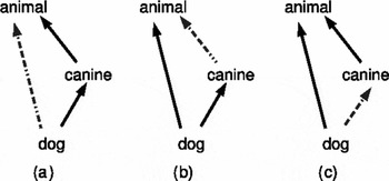
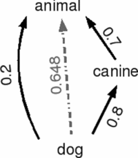
Yet, even if it is important, including confidence weights in knowledge repositories is not a trivial problem when considering semantic relations with structural properties as transitivity. In methods such as given by Pantel and Pennacchiotti (Reference Pantel and Pennacchiotti2006), it seems possible to easily include some initial values in the final resource, as these have been used for deciding whether the knowledge base should include a relation. Yet, when we need to combine these values in transitive relations, we need to be extremely careful on how these values have been estimated and computed. For example, if we discover from corpus analysis that ‘dog’ is a ‘canine’ and we already know that ‘canine’ is an ‘animal’ (see Figure 1(a)), using transitivity we can derive the induced relation, i.e. dog is an animal (the dashed arrow in Figure 1(a)). Yet, we cannot easily combine confidence weights if the nature of these weights is obscure.
Examples of relations derived by exploiting the transitivity.

The solution generally proposed for combining confidence weights is neglecting their nature. The final relation between two words has the same confidence weight as that of a reliable and controlled information. Even in probabilistic models (Snow et al. Reference Snow, Jurafsky and Ng2006), these reliable and unreliable information is mixed during the knowledge acquisition process. In these models, if ‘canine’ is an ‘animal’ (see Figure 1(a)) is in the original manually controlled network and ‘dog’ is a ‘canine’ has a high probability from the corpus observations, this latter is included in the knowledge base with the same degree of plausibility as that of ‘canine’ is an ‘animal’. Then, the induced relation ‘dog’ is an ‘animal’ has again the same degree of plausibility as that of manually controlled information. This is a loss of information, as the uncertainty of the relation ‘dog’ is an ‘animal’ is neglected.
3.2 Probabilistic definitions for concepts
As keeping and propagating uncertainty in transitive semantic networks is important, we propose an inductive taxonomy learning model, i.e. a probabilistic taxonomy learning model based on LSP that exploits transitivity during learning for determining confidence weights. Our model stems from the intuition that the LSP learning models contribute to probabilistic definitions of target concepts and that it is possible to combine these definitions to determine confidence weights derived in transitive networks. We hereafter observe how the LSP models contribute to the formal definitions of concepts; then we define what is a probabilistic definition, and, finally, describe how these probabilistic definitions can be used to determine two LSP inductive learning models: the intensional and the extensional model.
The LSP methods derive formal definitions for concepts (or, better, for words or word sequences) from texts. Extracting evidence from corpora suggesting that ‘dog’ is an ‘animal’ contributes to the definitions of ‘dog’ and ‘animal’. In the case of ‘dog’, the relation between ‘dog’ and ‘animal’ contributes to the intensional definition of ‘dog’ as it is stating that a ‘dog’ is an ‘animal’ with specific features. In the case of ‘animal’, this relation contributes, in a wide sense, to the extensional definitionFootnote 1 of ‘animal’. It is like we are giving one of the possible instancesFootnote 2 of the concept ‘animal’. These formal intensional and extensional definitions are often used to derive the similarity among words or concepts. Cotopy (Maedche and Staab Reference Maedche and Staab2002), a measure for determining similarity between concepts in two different semantic networks, uses exactly this information.
A probabilistic definition of a concept is an intensional definition associated with its induced probabilities. These probabilities are derived from the topology of transitive semantic networks mixing of existing knowledge and corpus estimated probabilities. In Figure 1, we report two kinds of arrows: the solid and the dashed ones. The solid arrow indicates relations derived from the existing structured knowledge repositories and from corpus analysis. The dashed arrow indicates the probabilities induced from the structure of the network. We want to describe the probability of the dashed relations using the probabilities of the solid ones. We call direct probabilities the first type and induced probabilities the second one.
Within the idea described above, we propose two models that derive induced probabilitic definitions from direct probabilities: the first exploits intensional definitions of concepts and the second exploits extensional definitions. We then name these two ways: the intensional inductive probabilistic model and the extensional probabilistic inductive model. To give an intuitive idea of our model, we use the example given in Figure 1.
The intensional inductive model exploits direct intensional definitions to derive an induced intensional definition. In Figure 1(a), we have, as direct information, the probabilities of the relations ‘dog’ is a ‘canine’ and ‘canine’ is an ‘animal’. From these two relations, we can derive the induced probability of the intensional definition of ‘dog’ is an ‘animal’. In this case we are exploiting and modeling the transitivity of a relation.
The extensional inductive model uses solid arrows, i.e. direct probabilities, to form extensional definitions of the concepts and compare the different extensional definitions for determining the final induced probability. In Figure 1(b), the relations ‘dog’ is an ‘animal’ and ‘dog’ is a ‘canine’ are used to form a very small part of the extensional definitions of ‘animal’ and ‘canine’, respectively. The idea is that these extensional definitions can be used to determine the similarity of ‘animal’ and ‘canine’. Then, we can derive the induced probability of the relation ‘dog’ is an ‘animal’. Using the same intuition, the relations ‘dog’ is an ‘animal’ and ‘canine’ is an ‘animal’ contribute to the extensional definition of ‘animal’ (see Figure 1(c)). Using all the other relations, we want to derive the induced probability of the relation ‘dog’ is a ‘canine’.
4 Inductive probabilistic model
In this section, we formalize the probabilistic definitions of concepts in an inductive probabilistic model. In Section 4.1, we define the two probabilistic models based on direct R i,j and inductive  i,j probabilistic events. In Section 4.2, we introduce three models for exploiting the probabilistic definitions of concepts within the inductive probabilistic model. Without loss of generality, we focus the examples and the prose on taxonomy learning. Yet, these models can be adopted for any transitive semantic relation.
4.1 Direct and inductive probabilistic models
As in Pantel and Pennacchiotti (Reference Pantel and Pennacchiotti2006) and Snow et al. (Reference Snow, Jurafsky and Ng2006)(Pantel and Pennacchiotti Reference Pantel and Pennacchiotti2006; Snow et al. Reference Snow, Jurafsky and Ng2006), we model the taxonomy learning problem as a binary classification task. Given a pair of words (i, j) and a vector of observed features  i,j, we want to build a binary classifier that determines if i is a j using i,j and gives the related confidence weight. As in Snow et al. (Reference Snow, Jurafsky and Ng2006), we see this problem in a probabilistic setting, as it gives us the possibility to determine the direct probability model as well as the induced probabilistic model.
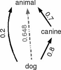
We here propose a model to exploit transitivity within probabilistic taxonomy learners that use LSP. Using LSP on a corpus, we can extract pairs of words in a given relation along with their reliability. These pairs of words and their reliabilities are directly observed. For example (see Figure 2), given the hyperonymy relation, we directly derive the reliabilities of the pairs ‘dog’ is a ‘canine’ (0.8), ‘canine’ is an ‘animal’ (0.7), and ‘dog’ is an ‘animal’ (0.2) (see the values on the solid arrows). If we now look at all these pairs together, we can observe that these words form a semantic network where transitive property holds. Even if the directly observed reliability of the pair ‘dog’ is an ‘animal’ is low (0.2), transitivity of the network suggests that this reliability should be higher (0.648). We exactly want to exploit the transitive network to induce the reliability of the relation between ‘dog’ and ‘animal’ (see the dashed arrow) using all the reliabilities of the involved pairs directly observed from the corpus. We then use a probabilistic setting where this composition of confidence weights can be better controlled.
Example of relations derived by exploiting transitivity.
In the direct probabilistic model, we define the direct events R i,j ∈ T, where T is the taxonomy. If R i,j is in T, i is a concept and j is one of its generalizations. For example, R dog,animal ∈ T describes that dog is an animal according to the taxonomy T. The learning problem in the direct setting is to determine the probabilities:
(1)


where E is a set of evidences extracted from corpus analysis, i.e. a set of i,j. We will hereafter refer to this probability as P(R i,j|E).
With some independence assumptions, we can rewrite (1) as P(R i,j|i,j), where i,j is the set of evidences for (i, j) derived from the corpus. These evidences are derived from the contexts where the pair (i, j) is found in the corpus. The vector i,j is a feature vector associated with a pair (i, j). For example, a feature may describe how many times i and j are seen in patterns like ‘i as j’ or ‘i is a j’. These among many other features are indicators of an is-a relation between i and j (as discovered in Hearst Reference Hearst1992).
These direct probabilities P(R i,j|i,j) only depend on what has been observed in the corpus for a particular pair of words (i, j). As transitivity has not been considered, P(R i,j|i,j) are initial probabilities of our probabilistic model for taxonomy learning. In the example of Figure 2 we have the following direct probabilities (where d = dog, a = animal, and c = canine): P(Rd,a|d,a) = 0.2, P(Rd,c|d,c) = 0.8, and P(Rc,a|c,a) = 0.7.
The inductive probabilistic model is the main innovation of our approach to taxonomy learning. Here we want to define an event space that models transitivity. We then introduce the events i,j and the related probability function:
(2)
This probability function should capture the fact that a decision on the pair (i, j) also depends on the transitive relations activated by (i, j). It is not always the case that these relations are activated by the existing taxonomy links. Yet, this inductive probability takes into account transitively related taxonomic links. We examine different models to exploit the transitive property of the R relation, and for each of these models we show that P(i,j|E) can be rewritten in terms of the involved P(Rh,k|E).
For example, we can compute the inductive intensional probability for the pair (dog,animal) in Figure 2. The inductive intensional probability P(d,a|E) can be computed as the probability of the event d,a = Rd,a ∪ (Rd,c ∩ Rc,a). This captures that the inductive event d,a is active when Rd,a happens or the joint event Rd,c ∩ Rc,a happens. Then, using the inclusion–exclusion property, the previous independence assumptions on the evidences E, and an independence assumption between R i,j, we can compute P(Rd,a ∪ (Rd,c ∩ Rc,a)|E) as

Given this initial idea, we formalize our inductive probabilistic models in next sections.
4.2 Three inductive probabilistic models
We propose three different methods for modeling induced probabilities. We call these intensional (Section 4.2.1), extensional (Section 4.2.2), and mixed models (Section 4.2.3). These three models exploit different definitions of the event i,j ∈ T. In the intensional model (Section 4.2.1), the event i,j ∈ T is represented as the event R i,j ∈ T and for any k all the alternative events Ri,k ∈ T and Rk,j ∈ T. In the extensional model (Section 4.2.2), the event i,j ∈ T is represented as the event R i,j ∈ T and for any k all alternative events Ri,k ∈ T and Rj,k ∈ T and all the events Rk,j ∈ T and Rk,i ∈ T. The last model, mixed model (Section 4.2.3), is a combination of the previous two models.
4.2.1 The intensional inductive model
In the intensional inductive model, we exploit direct probabilities to derive the induced probabilistic intensional definition PI(i,j|E). We evaluate this probability using the direct probability of R i,j ∈ T and the direct probabilities of having a transitive connection between i and j of two direct relations. For each possible node k, we then consider all alternative events Ri,k ∈ T and Rk,j ∈ T. We use a running example to illustrate the idea.
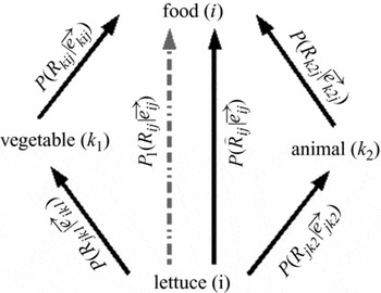
We suppose to have four elements in a network (see Figure 3): ‘lettuce’ (i), ‘food’ (j), ‘vegetable’ (k 1), and ‘animal’ (k 1). We empirically estimated the direct probabilities represented with bold arrows and want to determine the induced probability of the dashed arrow. Both the i − k 1 − j and i − k 2 − j paths offer some information to the final induced probability even if we expect that P(R i,k 1|E), i.e. the direct probability of ‘lettuce’ is a ‘vegetable’, is near to 1 and that P(R i,k 2|E), i.e. the direct probability of ‘lettuce’ is an ‘animal’, is near to 0. We compute the induced probability as the probability of alternative events that represents the sub-part of the network of direct events. In this case the induced probability is as follows:

Example of internal inductive model.

We can compute this probability using the inclusion–exclusion principle and some assumptions on the independence among events. The inclusion–exclusion principle gives the possibility of computing the probabilities of alternative events. Given n probabilistic events A 1, A 2,. . ., An in a probability space, the probability of the union of these events is as follows:

where AJ = ⋂i∈JAi. The probability PI(i,j|E) can then be rewritten as

Finally, assuming that the probabilities of the direct events, Rn,m, are independent, we can determine the probabilities of any of the joint events as products of the probabilities of the events, e.g.: P(R i,k 1 ∩ R k1,j|E) = P(R i,k 1|i,k 1)P(R k 1,j|k 1,j).
The general equation for the induced intensional probability is as follows:

where K = {k 1,. . ., kn} is the set of the intermediate nodes considered between i and j. As in the case of (3), we can compute this equation using the inclusion–exclusion principle as follows:

where RJ = ⋂k∈JRk. Each Rk is defined as R ε = R i,j and Rk = (Ri,k ∩ Rk,j) if k ≠ ε. Using the assumption that direct probabilities of Rm,n are independent, we can also rewrite P(RJ|E) as
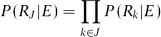
where P(R ε|E) = P(R i,j|i,j) and P(Rk|E) = P(Ri,k|i,k)P(Rk,j|k,j), if k ≠ ε.
4.2.2 The extensional inductive model
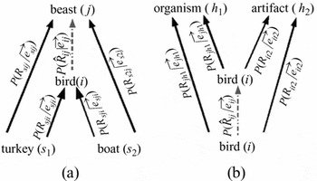
The extensional inductive model exploits the extensional definitions of the concepts to derive the induced probabilities. Figure 4 reports an example where two different models are adopted. The first model (see Figure 4(a)) uses the extensional definition of the two involved concepts, i.e. ‘turkey’ and ‘boat’, to determine the probability of the induced relation ‘bird’ is a ‘beast’, i.e. P(i,j|E). The similarity between the extensional definition of ‘bird’ (i) and ‘beast’ (j) should help in determining the probability of the relation between the two concepts. In the second model (see Figure 4(b)), ‘animal’ and ‘penguin’ contribute to the extensional definition of both organism and ‘artifact’. This should help in determining the probability P(i,j|E) of the induced event i,j. In the case of the reported running examples, the probability of the induced event is
(3)
These probability equations can be reduced using the inclusion–exclusion principle and the independence assumption between the direct events. We can then rewrite this equation as

Example of external inductive model.

We can finally write the general equation using the extensional probabilistic definitions of the concepts. In this model we mix the two previous models in one single equation. The probability P(i,j|E) of the induced event i,j is then rewritten in term of the probabilities of the direct events as follows:

4.2.3 The mixed inductive model
The mixed inductive model unifies the above-mentioned methods, considering both the intensional and the extensional probabilistic models. Formally,
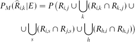
Similarly, the inclusion–exclusion principle can be used to evaluate the alternative probability for the mixed method.
The complete computation of the inductive probabilistic models presented in this section is unfeasible, as the computation of inclusion–exclusion principle is combinatorial with respect to the set of alternative events J. We then use an approximated computation derived from the method described in Kahn, Linial and Samorodnitsky (Reference Kahn, Linial and Samorodnitsky1993).
5 Estimating direct probabilities using SVD within logistic regression
The last problem we need to solve is how to estimate the direct probabilities, P(R i,j|i,j), using an initial knowledge base and a corpus to extract evidences for pairs (i, j). Once we have the direct probabilities, we can determine the induced probabilities with the models described in the previous sections. The second issue we want to address in this section is the problem of reducing the feature space in an unsupervised manner. We estimate the probabilities using the logistic regression model (Cox Reference Cox1958) and, as we will see, this gives a natural setting for using SVD as an unsupervised feature selection model.
In the rest of this section we will first introduce the logistic regression model (Section 5.1), then we will show how regression coefficients are estimated (Section 5.2), and finally describe how SVD is used as a feature selector in the logistic regression that estimates the probabilities of the model (Section 5.3). To describe this part we need to thoroughly examine the definition of the logistic regression.
5.1 Logistic regression
Logistic regression (Cox Reference Cox1958) is a particular type of statistical model for relating responses Y to linear combinations of predictor variables X. It is a specific kind of generalized linear model (see Nelder and Wedderburn Reference Nelder and Wedderburn1972), where its function is the logit function and the dependent variable Y is a binary or dicothomic variable, which has a Bernoulli distribution. The dependent variable Y takes value 0 or 1. The probability that Y has value 1 is a function of the regressors x = (1, x 1,. . .,xk).
The direct probability P(R i,j|i,j) falls in the category of probabilistic models, where the logistic regression, which can be applied as R i,j ∈ T, is the binary-dependent variable and i,j is the vector of its regressors.
We start from formally describing the logistic regression model. Given a binary stochastic variable Y and a generic stochastic variable X for the regressors, we can define p as the probability of Y to be 1 given X =  , i.e.

The distribution of the variable Y is a Bernoulli distribution. Given the definition of the logit(p) as
(4)
and given the fact that Y is a Bernoulli distribution, the logistic regression predicts that the logit is a linear combination of the values of the regressors, i.e.
(5)
where β0, β1,. . ., βk are called regression coefficients of the variables x 1,. . ., xk, respectively.
5.2 Estimating regression coefficients
The second issue is how to estimate the regression coefficients. This estimation can be done using the maximal likelihood estimation. The above logit definition generate a set of linear equations. The linear problem is then solved by introducing a pseudo-inverse matrix, the original matrix being usually rectangular and singular.
Once we have calculated the regression coefficients, we have the possibility of estimating a probability P(R i,j|i,j) given any configuration of the values of the regressors i,j, i.e. the observed values of the features.
The estimation of the β coefficients can be obtained as follows. Let us assume to have a multiset O of observations extracted from a corpus. Elements of the multiset are (y,i,j), where y = 1 if (i, j) is a positive case and y = 0 if (i, j) is a negative case. We can now derive the set E of all the different vectors i,j. For the sake of simplicity, we call these vectors  . For each ∈ E, we can use the maximum likelihood to estimate the initial probability P(Y = 1|) as the frequency of the pair (1, ) in O divided by the frequency of . For each ∈ E, we have a set of equations of this kind:
(6)
where m is the size of the feature space. This set of equations can be written as a linear equation system:
(7)
where Q is a matrix that includes a constant column of 1, necessary for the β0 of the linear combination of the values of the regression. The matrix is
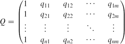
The set of equations in (7) is a particular case of multiple linear regression (Caron, Hospital and Corey Reference Caron, Hospital and Corey1998).
As Q is a rectangular and singular matrix, Q is not invertible and the system  = Qβ has no solutions. Yet, it is possible to use the principle of least square estimation. With this principle we can determine the solution β that minimize the residual norm, i.e.
(8)
This problem can be solved by the Moore–Penrose pseudoinverse Q + (Penrose Reference Penrose1995) that gives the following final equation:
(9)
It is important to remark that if the inverse matrix exists, then Q + = Q −1 and Q +Q, QQ + are symmetric.
5.3 Computing pseudoinverse matrix with SVD analysis
We can finally illustrate why it is natural to use SVD as feature selection in a probabilistic taxonomy learner. In the previous sections we described how the probabilities of the taxonomy learner can be estimated using logistic regressions and concluded that a way to determine the regression coefficients β is by computing the Moore–Penrose pseudoinverse Q +. Here we compute Moore–Penrose pseudoinverse Q + by using SVD in the following way (Penrose Reference Penrose1955). Given an SVD decomposition of the matrix Q = UΣVT, the pseudo-inverse matrix that minimizes the (8) is
(10)
The diagonal matrix Σ+ is the r × r transposed matrix of Σ having as diagonal elements the reciprocals of the Σ singular values  .
As we are using SVD in the computation of the pseudo-inverse matrix, we have the possibility of exploiting it as an unsupervised feature selection model. We can compute different approximations of the pseudo-inverse matrix. The algorithm for computing the singular value decomposition is iterative (Golub and Kahan Reference Golub and Kahan1965). The firstly derived dimensions are those with higher singular values. We can consider different k in order to obtain different SVD as approximations of the original matrix (10). We can define different approximations of the inverse matrix Q + as Qk +, i.e.

where Qk + is a matrix n by m obtained considering the first k singular values.
The property of the singular values computed by the Golub and Kahan (Reference Golub and Kahan1965) algorithm, i.e. δ1 ≥ δ2 ≥ ⋅⋅⋅ ≥ δr > 0, guarantees that the first k are bigger than the discarded ones. There is a direct relation between the informativeness of the i-th new dimension and the singular value δi. High singular values correspond to dimensions of the new space where examples have more variability, whereas low singular values determine dimensions where examples have a smaller variability (Liu Reference Liu2007). These latter dimensions can then be hardly used as efficient features in learning. The possibility of computing approximated versions of matrices gives a powerful method for feature selection and filtering as we can decide in advance the number of features or, better, linear combinations of original features we want to use.
6 An alternative approach: the iterativem Method
We illustrate here an existing state-of-the-art probabilistic model for taxonomy learning presented in Snow et al. (Reference Snow, Jurafsky and Ng2006). This probabilistic model is the only one based on LSP that intrinsically use the transitivity to expand the existing taxonomy. We will hereafter call this model iterative. We are interested in this model because it represents a valid alternative to ours. The iterative model, instead of determining induced probabilities, iteratively adds facts in the knowledge base changing the initial taxonomy.
In Snow et al. (Reference Snow, Jurafsky and Ng2006), the probabilistic taxonomy learning task is defined as the problem of finding a taxonomy  that maximizes the probability of observing the evidences E, i.e.

This maximization problem is solved with a local and iterative search. Each step maximizes the ratio between the likelihood P(E|T′) and the likelihood P(E|T), where T′ = T ∪ I(R i,j) and I(R i,j) are the added relations. This ratio is called multiplicative change Δ(N) and is defined as follows:
(11)
The main innovation of this model is the possibility of adding at each step the best relation {R i,j}, as well as all the relations induced from R i,j and the existing taxonomy T. Given the taxonomy T and the relation R i,j, the set I(R i,j) contains Ri,k if Rj,k is in T and contains Rk,j if Rk,i is in T. For example, given T and R dog,animal, if Ranimal,organism ∈ T, then I(R dog,animal) contains Rdog,organism. Moreover, given T and Rbird,beast, if Rturkey,beast ∈ T, then I(Rbird,beast) contains R turkey,beast.
The last important fact is that it is possible to demonstrate that the following equation holds:
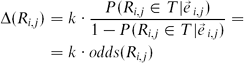
where k is a constant that will be neglected in the maximization process. This last equation gives the possibility of using the logistic regression in original form. The odds(R i,j) is strictly related to (4) of the logit(p), as presented in Section 5.1.
Our SVD-based logistic approach demostrates here all its efficiency. The iterative model requires the computation of the regression at each step. The more expensive part of the computation of the regression model that we have proposed is the computation of the pseudo-inverse matrix. This is computed only once for all the iterative process. In (9), the estimated  changes at each step because the estimated changes. The use of other regression methods, such as Support Vector Machines (Cortes and Vapnik Reference Cortes and Vapnik1995), is computationally unfeasible because they require to recompute the regression at each step.
7 Experimental evaluation
With this set of experiments, we want to determine the validity of our assumptions and our inductive probabilistic model for taxonomy learning. We first want to determine if keeping probabilities within the final knowledge base is better than taking strict decisions. To assess this claim we compare our direct probabilistic model with the state-of-the-art probabilistic model (i.e. the iterative model) presented in Section 6. We then analyze whether the way we are exploiting transitivity in the semantic relation is effective. We compare the direct model with the inductive model. Finally, we want to study if the SVD model for feature selection can be fully exploited within our probabilistic model.
The rest of the section is organized as follows. In Section 7.1, we describe the experimental setting: the corpus, the feature space, and the training and the testing set. In Section 7.2, we report and comment the results of the experiments. In Section 7.3, we qualitatively analyze the process of feature selection based on SVD.
7.1 Experimental set-up
To completely define the experiments we need to describe some issues: How do we define the taxonomy to replicate; which corpus have we used to extract evidences for pairs of words; and which feature space have we used.
As target taxonomy we selected a portion of WordNetFootnote 3 (Miller Reference Miller1995). Namely, we started from 44 concrete nouns divided into three classes: animal, artifact, and vegetable. For each word w, we selected the synset sw that generalizes with the class it belongs to. We then obtained a set S of synsets, and expanded the set to S′ by adding the siblings (i.e. the coordinate terms) for each synset in S. The set S′ contains 265 coordinate terms plus the forty-four original concrete nouns. For each element in S we collected its hypernyms, obtaining the set H. We then removed from the set H the top four classes: entity, unit, object, and whole. The set H contains seventy-seven hypernyms. For the purpose of the experiments we derived a taxonomy T from the previous sets and produced a set of negative examples T. The two sets have been obtained as follows. The taxonomy T is the portion of WordNet implied by O = H ∪ S′, i.e. T contains all the (s, h) ∈ O × O that are in WordNet. On the contrary, T contains all the (s, h) ∈ O × O that are not in WordNet. We then have 4,596 positive pairs in T and 48,354 negative pairs in T.
To obtain the training and the testing sets, we randomly divided the set T ∪ T in two parts Ttr ∪ Ttr and Tts ∪ Tts, respectively, the 70per cent and 30per cent of the original T ∪ T.
As a corpus we used the English Web as Corpus (ukWaC) (Baroni et al. Reference Baroni, Bernardini, Ferraresi and Zanchetta2009). This is a web-extracted corpus of about 2,700,000 web pages containing more than two billion words. The corpus contains documents of different topics, such as web, computers, education, public sphere, etc. It has been largely demonstrated that the web documents are good models for natural language (Lapata and Keller Reference Lapata and Keller2004).
We used a bag-of-n-gram feature space for implicitly modeling LSP. Features are words, bigrams, and trigrams. These n-grams represent specific LPS. Given a pair (i, j) ∈ T ∪ T, we build the related feature vector i,j using the contexts where the the words i and j appear in a window of at most five words. For each context of (i, j), the word sequence between i and j is used to increment the frequency of the related n-grams. For example, given the pair (car, vehicle), we can retrieve the context:
. . . to control the car as a motor vehicle and . . .
Considering only word sequences between the two target words, this context contributes to the features: as, a, motor, as a, a motor, and as a motor. These feaures are approximations of LSP.
7.2 Results
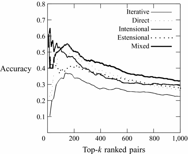
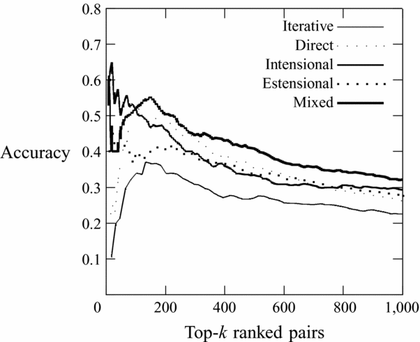
In the first set of experiments, we want to analyze the following two issues: (1) the relevance of the probability in the final knowledge base; and (2) the effectiveness of our inductive model. We evaluate the iterative, the direct, and the inductive probabilistic models on their ability of sorting the pairs. We have two classes of methods. The iterative model adds some pairs at each step. The direct and the inductive probabilistic models, instead, produce a sorting of pairs according to probabilities. We then compared the two methods in the following way. For the iterative methods, we plot the curve that relates the accuracy to the number of added pairs. The accuracy is computed as the number of correctly added pairs with respect to the added pairs. On the contrary, for the probabilistic models we plot the accuracies with respect to the ranked pairs. For this set of experiments, we used k = 100 for the pseudo-inverse matrix computation with SVD.
Results are reported in Figure 5. Firstly, we can observe that, after some initial steps, models that keep the probabilities are better than the models that make a decision at each step. The direct model already outperforms the iterative model. Then, the final knowledge base should keep the probabilities. The second observation is that the inductive (estensional, intensional, and mixed) models outperform the direct model. This shows that our way of encoding the transitivity is effective. Finally, among the inductive models, the mixed model is the best one. The mixed method exploits both intensional and estensional probabilistic definitions of concepts.
Accuracy of the top-k ranked pairs for the iterative, direct, and inductive probabilistic taxonomy learners.
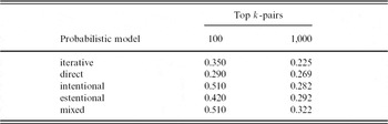
In order to take a closer look at the results of the first set of experiments, we reported the accuracies in Table 1. The table reports the accuracies for different probabilistic models for two different cuts of the sorted pair list. The second and the third columns report, respectively, the accuracies for 100 and 1,000 considered pairs. We used these two cuts to compute the statistical significance of the difference between the direct and the mixed models. To determine the statistical significance, we used the model described in Yeh (Reference Yeh2000)(Yeh Reference Yeh2000) as implemented in Pado (Reference Padó2006). We extended this latter for considering accuracies computed on sorted lists. According to these tests, the statistical significance is below 0.05 for both top k choices.
Accuracy of the different models at top 100 and 1,000 ranked pairs

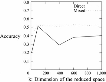
In the second set of experiments, we want to investigate the role of the feature selection performed using SVD on our probabilistic model. We analyze the accuracy on 100 considered pairs for different values of k, i.e. the number of considered dimensions for SVD used in the computation of the pseudo-inverse matrix. The plots of the direct and the mixed inductive probabilistic models are presented in Figure 6. For both models, the performances are stable or decrease after k = 100. An aggressive dimensionality reduction of the feature space does not negatively affect performances. Models with k = 100 features are computed much faster than the models with k = 1,000 features and performances are not significantly affected. The stability of the two curves suggests that, even by using the whole feature space, the performance cannot increase.
Accuracy of the direct and inductive probabilistic taxonomy learners with respect to SVD feature selection.

7.3 Qualitative analysis of dimensionality reduction
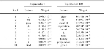
The experiments show that we can positively use dimensionality reduction of SVD within the computation of the pseudo-inverse matrix. We now want to analyze the first dimensions to understand which linear combination of the original features is relevant for the specific task of learning taxonomies using lexical patterns. As the decomposition algorithm that we are using sorts the eigenvectors according to decreasing eigenvalues, we will examine the first eigenvector that should be more significant and the eigenvector number 400. In Table 2, we present only some of these eigenvectors. We present the dimensions with the ten largest values. The first ten dimensions of the first eigenvector are presented in column 2 and 3. The first ten dimension of the 400th eigenvector are presented in column 4 and 5.
Two selected eigenvectors on the bag-of-n-grams

The first eigenvector is very interesting as it mixes many classical indicators of hypernymy, e.g. ‘,’, ‘be’, ‘&’, etc. These indicators appear with different relative weights in many of the first eigenvectors. It is worth noticing that the forms of the verb to be are present in the considered eigenvector. On the contrary, the eigenvector number 400 does not contain any relevant information related to the hypernymy phenomenon in the first positions. This qualitatively explains what has been shown by the experiments in the previous section. Many dimensions in the reduced space are totally irrelevant.
8 Conclusions and the future work
We presented a probabilistic taxonomy learning model that positively exploits transitivity. We demonstrated that keeping of the probability within the final knowledge base is extremely important for the performances of the learning method. We have also shown that our model positively exploits transitiveness, as the inductive model outperforms the direct model. Finally, we have demonstrated that SVD can be used as a natural feature selection model within the probabilistic taxonomy learning models.
In the future, we want to extend the model to consider feature spaces more complex and richer than bag-of-words. We believe this will boost the performances of our model. We plan to test our model for different transitive semantic relations, such as part-of, cause–effect, entailment, etc. Moreover, we want to extend the model to consider other structural properties of semantic networks