2.1 Facility and particle image velocimetry instrumentation

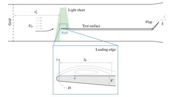
All measurements were carried out in an open-return, suckdown wind tunnel over a flat aluminium plate (figure 1). The tunnel consists of a bell-mouthed inlet, settling chamber (with a coarse honeycomb and a fine woven-mesh screen), contraction, working section ( $300~\text{mm}\times 300~\text{mm}\times 1000~\text{mm}$ ), diffuser (with two screens) and four axial fans in parallel. The background turbulence level $T_{ub}$ in the empty working section is 0.45 %.

Figure 1.

Cross-sectional view of the working section, grid, test plate and PIV set-up (not to scale). The zoom view shows the geometry of the leading edge.

The plate is 295 mm wide and is made up of three sections: (i) an asymmetrical leading edge, the underside of which is tapered at $5^{\circ }$ from the plate proper (10 mm thick) to a semi-cylindrical nose of diameter $D=2~\text{mm}$ ; (ii) a long test surface, which is smoothly conjoined to the leading edge; and (iii) a hinged trailing-edge flap (85 mm long), which allows the incidence of the approaching free stream to be manipulated indirectly. When the flap is set to a low angle $\unicode[STIX]{x1D709}$ , a separation bubble of time-mean length $l_{R}$ will appear on the test surface. The full plate is 920 mm long, excluding the flap.

The PIV system (from TSI Inc.) comprised a 200 mJ pulsed Nd:YAG laser, an 11 megapixel charge-coupled device camera (with a Sigma $f/2.8$ 105 mm prime lens) and a commercial fog machine. The field of view (FoV) in the laser light sheet ( $x$ – $y$ ) plane was $42~\text{mm}\times 28~\text{mm}$ and was offset by 10 mm from the centreline of the plate to accommodate the focus distance to the lens. In each case, 1000 image pairs were captured at a frequency of 0.55 pairs per second, as limited by the write speed of the storage drive. The vector field was later computed recursively across a rectangular grid of interrogation spots (down to a spacing of $93~\unicode[STIX]{x03BC}\text{m}$ per vector) using the second-order deformation algorithm in TSI Insight. This algorithm is based upon the iterative multigrid method of Scarano (Reference Scarano2002) and is particularly effective against in-plane velocity gradients. Each field was also corrected for mild pincushion distortion from the lens, although the effect was negligible.

Total uncertainty in PIV velocity measurements depends upon both bias (due to equipment and calibration) and random errors (which vary across the flow field according to local image quality, fluid strain and rotation, particle-image characteristics, etc.). The former being known, the latter were estimated using the Insight implementation of the peak ratio method (Charonko & Vlachos Reference Charonko and Vlachos2013). In case A, for example, the total standard uncertainty in the unsteady region to the rear of the bubble was typically 5–10 %, whereas in the laminar shear layer (and external stream), it was 1–3 %. Amid the upstream part of the bubble, it rose to 20–25 %, but here we were concerned only with the streamwise direction of the flow (to deduce the reattachment point) and not its magnitude.

Figure 2.

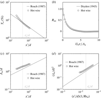
Characteristics of the grid-generated FST. Panels (a,c,d) show the development of the streamwise turbulence intensity $T_{u}$ , integral length scale $\unicode[STIX]{x1D6EC}_{u}$ and Taylor microscale $\unicode[STIX]{x1D706}_{u}$ , respectively, with distance $x^{\prime }/d$ behind the grid. Panel (b) shows the correlation function $R_{uu}$ at the location of the leading edge ( $x_{L}^{\prime }/d=47.3$ ), with only every 25th data point shown for clarity (the original data are very highly resolved).

2.2 Free stream turbulence

For case B, FST was generated upstream of the plate by means of a 2 mm thick perforated grid. The bars of the grid are $d=7~\text{mm}$ wide and spaced evenly at a mesh length of $M=26~\text{mm}$ . The turbulence was characterised in the empty working section of the tunnel with an AN-1005 hot-wire anemometer (from AA Lab Systems) and a 55P11 single-wire probe (from Dantec) that had been calibrated in situ beforehand against a Pitot-static tube using King’s law. Fluctuations in ambient temperature were corrected by the method of Kanevče & Oka (Reference Kanevče and Oka1973).

The decay of streamwise turbulence intensity $T_{u}$ with dimensionless distance $x^{\prime }/d$ behind the grid is shown in figure 2(a). For comparison, the data are plotted against the power-law correlation from Roach (Reference Roach1987),

with $A=1.13$ (Roach’s value for this grid type and Reynolds number); $\sqrt{\,\overline{u^{\prime 2}}}$ is the root-mean-square level of the streamwise fluctuations $u^{\prime }$ , where the overline denotes the time-averaging operation. After an initial settling region, the measured turbulence decays at approximately the same rate as Roach’s line. The leading edge ( $L$ ) of the plate was therefore positioned at the end of this region ( $x_{L}^{\prime }=331$  mm or $x_{L}^{\prime }/d=47.3$ ) in order to avoid any development effects near the grid. Figure 2(b) shows the streamwise correlation function at this location, computed as an autocorrelation of the $u^{\prime }$ signal or

and this matches Dryden’s (Reference Dryden, Friedlander and Topper1943) function for isotropic turbulence,

quite closely. Note that $R_{uu}$ has been plotted against the dimensionless quantity $U_{0}\unicode[STIX]{x1D70F}/\unicode[STIX]{x1D6EC}_{u}$ , where $\unicode[STIX]{x1D70F}$ is the time-lag variable (the product $U_{0}\unicode[STIX]{x1D70F}$ is therefore equivalent to the streamwise separation distance in a two-point correlation) and $\unicode[STIX]{x1D6EC}_{u}$ is the streamwise integral length scale, which was estimated by integration of $R_{uu}$ with respect to $\unicode[STIX]{x1D70F}$ as

The upper limit $\unicode[STIX]{x1D70F}_{L}$ was defined as the first point at which $R_{uu}=0.02$ to prevent any ‘noisy’ oscillations that might appear at large $\unicode[STIX]{x1D70F}$ from affecting the integral sum. This follows from the study of O’Neill et al. (Reference O’Neill, Nicolaides, Honnery and Soria2004), who used the first zero-crossing point of $R_{uu}$ .

The streamwise growth of $\unicode[STIX]{x1D6EC}_{u}$ is shown in figure 2(c). Roach’s (Reference Roach1987) universal correlation for all grid types,

is also shown. We note that his choice of growth exponent (0.5) was a general assumption, made for reasons given in his paper, and that the leading coefficient (0.2) was determined by regression to a multitude of datasets. Whilst the agreement is therefore reasonable given the generality of the correlation, we find from an optimised curve fit to our data that the present exponent is actually 0.37, and the leading coefficient 0.45. This is more consistent with the data of Kurian & Fransson (Reference Kurian and Fransson2009), who find an exponent of 0.33. Nonetheless, the correlation provides the requisite benchmark for comparison.

The Taylor microscale $\unicode[STIX]{x1D706}_{u}$ provides a measure of the smallest energetic eddies in the flow, i.e. anything smaller falls into the viscous dissipation range. It is defined by

In this work, $R_{uu}$ was sufficiently well resolved at small $\unicode[STIX]{x1D70F}$ for $\unicode[STIX]{x1D706}_{u}$ to be approximated using a simple finite difference. The computed results are plotted in figure 2(d) alongside Roach’s (Reference Roach1987) corresponding correlation,

which may be obtained from theory and (2.1). Note that $Re_{d}=U_{0}d/\unicode[STIX]{x1D708}$ is the bar Reynolds number of the grid. Despite a small vertical offset, the growth exponent here compares favourably to the data after the initial settling region.

These characteristics suggest overall that the turbulence is well behaved and, on the basis of figure 2(b) in particular, sufficiently isotropic for this work. PIV data from case B also show that the mode of the ratio $\overline{u^{\prime 2}}/\overline{v^{\prime 2}}$ in the free stream is approximately 1.04.

3.1 The flap effect

For attached boundary-layer experiments on plates, it is imperative that separation is prevented at the leading edge. One common method is to use an asymmetrical leading-edge section in conjunction with a raised trailing-edge flap: the leading edge provides a smooth blend from the plate proper (usually quite thick for structural reasons) to a finely rounded nose, and the flap provides the circulation necessary for the flow to attack the plate at negative incidence. This ensures that the stagnation point remains firmly anchored to the nose (Hernon, Walsh & McEligot Reference Hernon, Walsh and McEligot2007) so that separation is avoided. The attendant boundary layer might require a virtual origin for proper scaling, but under constant-pressure conditions will usually follow Blasius’ solution after a short initial leading-edge development length.

Figure 3.

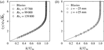
Velocity profiles of the attached, laminar boundary layer that grows on the test surface when $\unicode[STIX]{x1D709}=45^{\circ }$ and the external velocity $U_{\infty }\simeq 4.9~\text{m}~\text{s}^{-1}$ . Panel (a) shows growth along the centreline, and panel (b) the profiles 25 mm on either side of this line (in the cross-stream or $z$ direction) at $Re_{x}=U_{\infty }x/\unicode[STIX]{x1D708}=57\,700$ in order to demonstrate spanwise homogeneity. The shape factor $H_{12}$ for these profiles is in the range 2.53–2.60, confirming that the streamwise pressure gradient is small (Blasius’ profile yields $H_{12}=2.59$ ). Note that a virtual origin of $+10~\text{mm}$ , a downstream shift, has been applied; $x$ therefore extends from the new coordinate origin.

Table 1.

Experimental parameters in each case.

The present plate was designed in accordance with similar guidelines from Roach & Brierley (Reference Roach and Brierley1992). Attached flow is obtained when the elevation angle $\unicode[STIX]{x1D709}$ of the flap reaches approximately 45 $^{\circ }$ ; in this configuration the boundary layer that grows downstream is laminar and matches Blasius’ scaling well (figure 3). 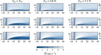But as the flap is lowered from $\unicode[STIX]{x1D709}=45^{\circ }$ , the circulation strength decreases and the approach angle of the incident flow increases. Eventually the flow can no longer remain attached and separates from the nose to form a bubble of reverse flow. The effect is demonstrated in figure 4 (reproduced from Stevenson et al. Reference Stevenson, Walsh, Nolan and Davies2014) for three flap settings and FST intensities, albeit at a slightly lower Reynolds number than the present work.

Figure 4.

Contours of the mean absolute velocity magnitude $|\overline{V}|$ at the leading edge for nine separated flows (from Stevenson et al. Reference Stevenson, Walsh, Nolan and Davies2014). Reynolds number $Re_{D}=480\pm 20$ . Isolines of $\overline{u}=0$ are shown by white lines. The profile of incident vectors at $x=-6$  mm has also been included in each case. Axes units are millimetres.

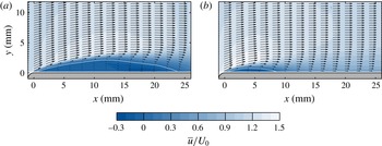
The flap setting of $\unicode[STIX]{x1D709}=0^{\circ }$ was chosen for further study at two levels of FST. Details of these experiments, including the turbulence characteristics at the leading edge, are provided in table 1, and contours of mean velocity are presented in figure 5. As described previously, the action of the flap (or lack thereof) causes the incident flow to approach at an elevated angle such that separation is forced at the leading edge. A thin band of shear, really a free shear layer, subsequently develops between the separated, high-velocity fluid in the free stream and the underlying low-velocity region, which at this Reynolds number is strong enough to initiate roll-up and ultimately the transition to turbulence. The flow then reattaches to form a recirculating separation bubble that is driven continuously by the shear. Under elevated FST (case B), the bubble shortens almost threefold from 24.4 mm to 8.9 mm. Its centre of ‘rotation’ (in terms of $l_{R}$ ) is also brought forward, whilst the maximum backflow velocity remains approximately the same at $\overline{u}/U_{0}\simeq -0.3$ (the importance of this is discussed in § 3). That FST tends to shrink or even eliminate separation bubbles has been observed by several workers at high Reynolds numbers (e.g. Kalter & Fernholz Reference Kalter and Fernholz2001) and is usually attributed to the effects of enhanced entrainment. At the present low Reynolds number, the shrinkage effect results primarily from an accelerated transition of the shear layer (§ 3.2).

Figure 5.

Contours of the streamwise velocity $\overline{u}/U_{0}$ in each case. Isolines of $\overline{u}/U_{0}=0$ are shown by white lines. Coarse vector profiles of the mean flow have also been overlaid.

3.2 Fluctuations in the shear layer

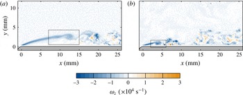
Perhaps the clearest overall perspective of the bubble dynamics is provided by the field of instantaneous spanwise vorticity (figure 6). In each case, the development of the flow is observed to consist of four essential parts: (i) the establishment and growth of the free shear layer from the point of separation, as shown by the smooth band of (diminishing) negative vorticity that extends from the leading edge; (ii) the onset of roll-up near the crest of the shear layer, which usually manifests as a circular patch of nearly constant negative vorticity (actually vortex roll-up, as later shown in the flow fields of figures 10 and 11); (iii) breakdown of the shear layer to turbulence, during which a wide range of three-dimensional motions – revealed by the divergence field, though not shown – start to appear; and finally (iv) reattachment to the wall to form a new turbulent boundary layer. Further, figure 6(b) shows that the point of roll-up in the shear layer is significantly advanced in case B. This mechanism, in combination with the enhanced spreading and mixing that take place naturally under elevated FST (Bearman & Morel Reference Bearman and Morel1983), serve to bring forward the first point of reattachment, and this in turn accounts for the observed reduction in the length of the bubble.

Figure 6.

Contours of the spanwise vorticity component $\unicode[STIX]{x1D714}_{z}$ for an instantaneous flow field in each case. The black windows are later referenced in figures 10 and 11.

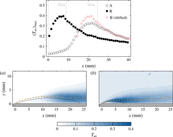
In a time-mean sense, the unsteadiness associated with the transition process is well described by the two-component turbulence intensity $T_{uv}$ (figure 7), defined as

where $u^{\prime }=u-\overline{u}$ and $v^{\prime }=v-\overline{v}$ are the Reynolds-decomposed velocity fluctuation components. Sasaki & Kiya (Reference Sasaki and Kiya1985) also suggest that the locus of maximum turbulence intensity may be used to identify the centreline, and hence trajectory, of a separated shear layer, and so this has been added to each contour in figure 7. We note that the laminar portion of the shear layer is reasonably steady in each case, and consequently the time-mean (figure 5) and instantaneous (figure 6) paths match one another quite well. An accompanying line plot of $(T_{uv})_{max}$ has also been included in the top panel of figure 7. This shows the familiar ‘growth–peak–decay’ behaviour that is fundamental to the transition process; Fransson, Matsubara & Alfredsson (Reference Fransson, Matsubara and Alfredsson2005) present a similar plot for the case of attached bypass transition, as do Langari & Yang (Reference Langari and Yang2013) for their separated flow under elevated FST.

Figure 7.

(a,b) Contours of $T_{uv}$ in each case, with orange dots marking the loci of $(T_{uv})_{max}$ at every 10th streamwise grid point. Isolines of $\overline{u}/U_{0}=0$ are shown in black. A corresponding line plot of $(T_{uv})_{max}$ along each locus has been included in the top panel. Note that the abscissa limits on the line plot extend to the extreme right-hand edge of the PIV field of view (not required by other plots) to show the decay phase.

In case B, initial events are clearly accelerated, in that $(T_{uv})_{max}$ grows more rapidly and reaches its peak much earlier, but downstream the decay rates turn out to be very similar. This has been illustrated by re-plotting the data for case B at a distance of 14 mm downstream but in light-coloured solid circles. Note that the shift is comparable to the difference between the time-mean bubble lengths ( $=15.5~\text{mm}$ ). The similarity could suggest that some form of ‘shear sheltering’ effect, provided by efflux from the bubble – see Hunt & Durbin (Reference Hunt and Durbin1999) for the original idea and Kalter & Fernholz (Reference Kalter and Fernholz2001) in this context – shields the reattaching boundary layer, so that after a certain point its development no longer depends upon the external turbulence. But whilst an interesting possibility, certainly from the perspective of boundary-layer control, one cannot draw firm conclusions without further data in the downstream direction.

Figure 8.

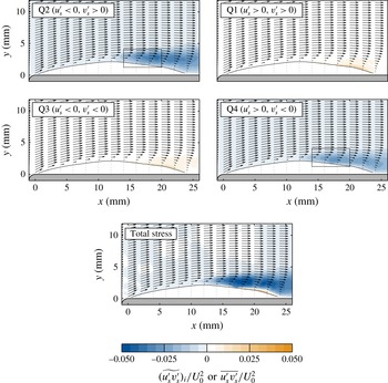
Contours of the stress contribution $\widetilde{(u_{s}^{\prime }v_{s}^{\prime })_{i}}/U_{0}^{2}$ from each quadrant in case A (excluding the bubble region). Total Reynolds stress $\overline{u_{s}^{\prime }v_{s}^{\prime }}/U_{0}^{2}$ is shown in the bottom panel. Isolines of $\overline{u}/U_{0}=0$ are shown in black. Coarse profiles of the corresponding mean vector field have also been overlaid.

Figure 9.

Contours of the stress contribution $\widetilde{(u_{s}^{\prime }v_{s}^{\prime })_{i}}/U_{0}^{2}$ from each quadrant in case B (excluding the bubble region). Total Reynolds stress $\overline{u_{s}^{\prime }v_{s}^{\prime }}/U_{0}^{2}$ is shown in the bottom panel. Isolines of $\overline{u}/U_{0}=0$ are shown in black. Coarse profiles of the corresponding mean vector field have also been overlaid.

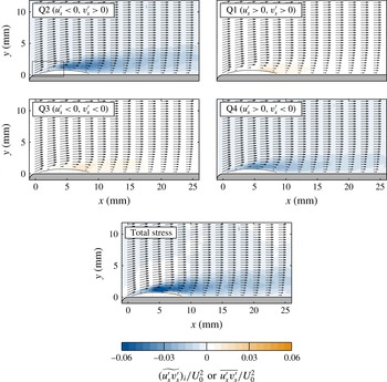
We have found the method of Reynolds-stress decomposition, often known simply as quadrant analysis, to be particularly effective in describing the physical nature of the fluctuations within the shear layer. The idea was first introduced by Lumley (Reference Lumley1970) and is useful in almost all fluctuating shear flows for identifying the main contributors to momentum transfer. For discrete data, the total Reynolds stress $\overline{u^{\prime }v^{\prime }}$ is usually calculated as the time average of contributions from the instantaneous fluctuation product $u^{\prime }v^{\prime }$ , which can be either positive or negative depending on the individual signs of $u^{\prime }$ and $v^{\prime }$ . If $u^{\prime }v^{\prime }>0$ , then $u^{\prime }$ and $v^{\prime }$ are either both positive or both negative; the product therefore belongs in quadrant 1 or 3. If $u^{\prime }v^{\prime }<0$ , then the product belongs in quadrant 2 or 4. ‘Quadrant’ (denoted Q) here has its usual meaning: one of the four sectors in the Cartesian $u^{\prime }$ – $v^{\prime }$ plane. At each point in the flow, the total stress $\overline{u^{\prime }v^{\prime }}$ can therefore be decomposed into contributions $\widetilde{{u^{\prime }v^{\prime }}_{i}}$ from each quadrant $i$ as

where

Here $N$ is the total number of measurement samples, and $N_{i}$ is the number that lie in quadrant $i$ , i.e. $N=\sum N_{i}$ . Now in the case of the boundary layer on a flat surface, whose time-mean streamlines are virtually parallel, quadrant analysis at each point is usually carried out in the fixed wall coordinate system ( $x$ – $y$ in this work) so that the sense of the fluctuations is clear. For curved shear layers like the present, however, it is perhaps more appropriate to work in a local system aligned with the mean streamlines, the main requirement being that the flow display a clear direction of development (Castro & Haque Reference Castro and Haque1987). We have therefore decided to adopt this approach. The velocity fluctuations in this system have been distinguished by a subscript ‘ $s$ ’ for ‘streamline’, and in any subsequent reference to a ‘Reynolds stress’ the use of this system is implied. Note that the bubble of reverse flow has been omitted; the flow direction here is not amenable to the analysis.

Figures 8 and 9 show contours of the quadrant-decomposed Reynolds stress around the bubble in cases A and B, respectively. All stresses are practically zero in the laminar part of the shear layer; those in Q1 and Q3 remain that way for most of the bubble. However, there exists a thin band of orange downstream that corresponds (if one envisages the orientation of a set of ‘quadrant axes’ in this region), for Q1 and Q3, respectively, to the recirculation of relatively low-speed (reversing) fluid back into the bubble and the deflection of relatively high-speed fluid into the new wall layer. This is one of the key processes of reattachment.

Figure 10.

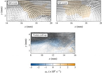
Fields of instantaneous absolute velocity in case A. The lower panel corresponds to the window on the left-hand contour in figure 6 and shows roll-up of the shear layer. The upper panels show typical Q4 and Q2 events from within the windows on the corresponding contours in figure 8. Each has been contoured by a logical function that is true (orange) wherever that event is detected (in streamline or ‘ $s$ ’ coordinates).

At $x\simeq 12~\text{mm}$ in case A, which also coincides with the location at which $(T_{uv})_{max}$ starts to rise considerably, the total stress increases due to large negative contributions from events in Q4 and Q2. These events broadly correspond to the movement of relatively high- and low-speed fluid towards and away from the wall, respectively, although those in Q2 can still correspond physically to downflow. Case B is quite similar in that contributions from Q2 and Q4 dominate the total stress in the latter part of the bubble – but particularly interesting is that the laminar part of the shear layer ( $0<x<2.5~\text{mm}$ ) also exhibits significant activity in these quadrants. We return to this point shortly.

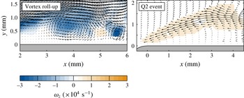
Attention is first drawn to the vorticity plots in figures 10 and 11, which show roll-up of the shear layer in each case. Most experimental and computational studies on separation on blunt or round-nosed plates report the presence of these KH vortices; the high-resolution direct numerical simulation of Lamballais et al. (Reference Lamballais, Silvestrini and Laizet2010) is one particularly lucid example and is qualitatively identical to what is seen here. Under elevated FST of the present magnitude, the only study of which we are aware is that of Langari & Yang (Reference Langari and Yang2013), who also suggest that concentrated regions of vorticity emerge near the leading edge, although not at the usual KH frequency. We do not here have the temporal resolution to comment upon shedding frequency but can confirm that distinct vortices, as shown in figure 11, are present in most of the instantaneous realisations of case B during the accelerated transition of the shear layer.

Figure 11.

Fields of instantaneous velocity in case B. The left-hand panel corresponds to the window on the right-hand contour in figure 6 and shows roll-up of the shear layer in terms of the absolute velocity field ( $u$ , $v$ ). The right-hand panel shows a typical Q2 event, as a Reynolds-decomposed fluctuation, from the window in the upper left-hand contour of figure 9. The fluctuation has been contoured by a logical function, as in figure 10.

Figure 12.

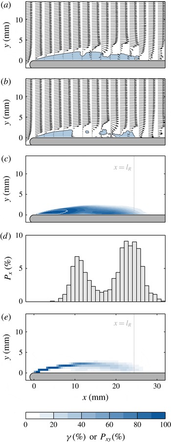
Reattachment and reverse-flow behaviour in case A. The instantaneous vector fields in panels (a) and (b) are contoured by isolines of $u=0$ and the regions they separate. The resulting distribution of the reverse-flow intermittency parameter $\unicode[STIX]{x1D6FE}$ (the probability that $u<0$ at each point) is shown in panel (c), with a white line to denote $\unicode[STIX]{x1D6FE}=99$  %. In panel (d), a histogram of the reattachment point for the separation isoline is plotted in 1 mm bins. Last, in panel (e), the field has been divided into tiles of $0.25~\text{mm}\times 0.25~\text{mm}$ , each of which is coloured according to the probability $P_{xy}$ that the separation isoline will lie within it during a realisation, i.e. it is a joint probability distribution function.

It was shown in figures 8 and 9 that in both cases the contributions to the total Reynolds stress from Q2 and Q4 were particularly strong over the latter half of the bubble. From a careful study of the individual vector fields in this region, it was subsequently found that the main transfer of momentum in Q4 results clearly from the type of event shown in the upper left-hand panel of figure 10, which shows fluid from upstream becoming entrained by a ‘residual’ KH vortex and diverted forcibly towards the wall at a speed greater than the mean. The corresponding region that actually generates Q4 stress (in streamline coordinates) has been contoured in orange. Note from figures 8 and 9 that the associated stress contribution is strongest at points that, on average, are: (i) far enough from the wall to experience entrainment only from the top side of the vortices; and (ii) far enough downstream for the vortices to have evolved to a sufficient strength. In fact, the mechanism is quite similar to the one suggested by Tafti & Vanka (Reference Tafti and Vanka1991) in their numerical study and is presumably responsible for driving reattachment processes at the rear of the bubble. In the upper right-hand panel of figure 10, a typical Q2 event – an energetic upwelling of fluid – is shown. Whilst this particular event appears to have been induced by the rising side of a vortex, many in Q2 seem incoherent and do not.

For case B, it was also noted previously that the total stress in the laminar part of the shear layer – before $(T_{uv})_{max}$ reaches its peak – receives strong negative contributions from both Q2 and Q4. The right-hand panel in figure 11 shows one such event from Q2: a slender, yet highly coherent, negative $u_{s}^{\prime }$ fluctuation (hence positive $v_{s}^{\prime }$ ) that spans the full length of the laminar shear layer until the onset of roll-up. Similar positive fluctuations in Q4 have also been observed. In the side view shown here, these structures are reminiscent of the laminar streaks that are usually observed in pre-transitional boundary layers (Nolan & Walsh Reference Nolan and Walsh2012) and upstream of laminar separation bubbles (Taniguchi, Sakai & Funazaki Reference Taniguchi, Sakai and Funazaki2012) under elevated FST. The vorticity isosurfaces presented by Langari & Yang (Reference Langari and Yang2013) for a transitional free shear layer under 5.6 % FST also appear to show corrugated fluctuations of a similar nature.

3.3 The reattachment process

Finally, we consider the reattachment process of the shear layer and the related question of ‘flapping’. Figure 12(a,b) shows the reverse-flow behaviour for two instantaneous realisations of case A (only this case is considered due to resolution limits near the wall). Each field has been contoured by isolines of $u=0$ into logical regions of forward ( $u>0$ , white) and reverse ( $u<0$ , blue) flow. Profiles of the instantaneous vector field have also been overlaid. The isoline is intended here as a device to reveal both the separation trajectory of the laminar part of the shear layer, with which it will move in tandem, and its unsteady reattachment behaviour downstream.

A common definition for the instantaneous reattachment point of a free shear layer is the last downstream location at which the skin friction is zero. This also corresponds to the last intersection between any isoline of $u=0$ and the wall. But in this flow, whilst there are times when the region of reverse flow at the leading edge constitutes a singular whole, as in figure 12(a), there are also times when it is fragmented into one or more isolated parts, as in figure 12(b). Some (or all) of these parts have no direct connection to the separating shear layer itself. By the usual definition, then, both of these bubbles would be regarded as having about the same instantaneous length, when in fact the main bubble of reverse flow at the leading edge differs in length by almost a factor of 3. We therefore suggest that the downstream end of the isoline that extends unbroken from the separation point, termed here the ‘separation isoline’, be used to define the true location of instantaneous reattachment (see also Castro Reference Castro2005). Figure 12(c) shows the associated time-mean distribution of the reverse-flow intermittency parameter $\unicode[STIX]{x1D6FE}$ , which confirms that the separation isoline always bounds a region of reverse flow at the leading edge.

Figure 12(d) shows the probability distribution $P_{x}$ of this first reattachment point; it is distinctly bimodal. Both of the peaks are quite well defined, implying that the main bubble spends most of its time in either a ‘short’ or ‘elongated’ state. The upstream peak, corresponding to the former, coincides with the location of marked fluctuation growth ( $x\simeq 10$  mm) in figures 6–8, which suggests that this reattachment scenario may be linked to roll-up of (and shedding from) the laminar shear layer. The downstream peak, synonymous with elongated bubbles of the type shown in figure 12(a), is located very near the time-mean reattachment point. These bubbles must form by continuous re-injection from downstream, as described by Eaton & Johnston (Reference Eaton and Johnston1982), by means of either (i) a very large structure, possibly a single vortex, or (ii) other smaller-scale structures. The former is unlikely in this case, however, because we have not observed any structures with a streamwise scale of the order of the distance between the peaks ( $\simeq l_{R}/2$ ). Q4 vortex events (figure 10) would seem to provide one logical physical basis for the reattachment process that causes this peak, but examination of the vector fields is inconclusive. These events do not appear to be consistently associated with elongated bubbles in the present, stationary reference frame.

An even fuller picture of the main bubble is provided by a joint probability distribution function $P_{xy}$ of the location of the separation isoline between realisations. This is shown in figure 12(e). The diffusion of colour reveals horizontal and (slight) vertical movements that cause the reattachment point to jump along the wall in accordance with the two ‘touchdown’ peaks on the histogram. Such wide-scale motions are a well-known feature of turbulent flows with low-frequency flapping (Eaton & Johnston Reference Eaton and Johnston1982; Yang & Voke Reference Yang and Voke2001). This fact, in combination with the absence (at present) of a definitive connection between regular KH shedding and the secondary peak, suggests that this flow may also be liable to a flapping motion involving the ‘elongated’ bubble, with the possibility of an associated global shedding mode (see Castro Reference Castro2005) – the maximum backflow velocity ( $\simeq 0.3U_{0}$ ) and Reynolds number (790) are certainly high enough.