1 Introduction
Eliciting truthful answers from respondents on sensitive issues is a difficult problem in surveys. When surveyors ask respondents these questions directly, some respondents may not be willing to answer truthfully or may even refuse to answer. To address this problem, several survey techniques have been developed and have gained popularity among political scientists and sociologists, such as list experiments (item count technique), randomized response techniques, and endorsement experiments. In political science, scholars have conducted and analyzed list experiments on various topics involving sensitive behaviors or attitudes (early works include Kuklinski, Cobb, and Gilens Reference Kuklinski, Cobb and Gilens1997 on racial prejudice; Kane, Craig, and Wald Reference Kane, Craig and Wald2004 on religion; Streb et al. Reference Streb, Burrell, Frederick and Genovese2008 on gender; Corstange Reference Corstange2009 on turnout; and Holbrook and Krosnick Reference Holbrook and Krosnick2010 on voting rights; see Section 3.2 for a list of recent works).
List experiments are intended to eliminate the direct association between a respondent’s answer and his or her attitude toward the sensitive item by including a few nonsensitive items (“control items”).Footnote 1 By doing so, list experiments give respondents the opportunity to provide truthful answers to the question while not revealing their attitudes toward the sensitive issue. Even though researchers do not gain knowledge about individual respondents’ preferences toward the sensitive issue, researchers can obtain the proportion of the population whose truthful responses are affirmative to the sensitive issue under some important assumptions. In their research on list experiments, Imai (Reference Imai2011) and Blair and Imai (Reference Blair and Imai2012) formulate the following two assumptions: (1) the inclusion of the sensitive item has no effect on respondents’ latent answers to the control items; (2) respondents give truthful latent answers to the sensitive item.Footnote 2 The analysis of list experiments depends crucially on these two assumptions, with the first assumption called “no design effect” and the latter referred to as “no liars”. The standard estimator is the difference between the average response from treated respondents and that from control respondents. The estimator is simple, intuitive, and unbiased under the assumptions of no design effect and no liars.
The no liars assumption is strong and may fail in many list experiments. In particular, a treated respondent who favors all or a large number of control items and the sensitive item may be reluctant to answer truthfully, as it reveals with certainty or a high probability that the respondent favors the sensitive item. In a recent study, Rosenfeld, Imai, and Shapiro (Reference Rosenfeld, Imai and Shapiro2016) find that their list experiment underestimates high incidence behavior in the context of a telephone interview. One possible explanation for this observation is that some respondents give untruthful answers for the sensitive item. Statistical tests are useful to detect certain forms of violations, but they usually look at the no design effect assumption, may lack power, or only examine a small subset of respondents. In this paper, I relax the no liars assumption, and in order to do so, maintain the no design effect assumption and focus on behaviors or attitudes with one-sided sensitivity.
I first illustrate which quantities concerning the proportions of different types of respondents are identifiable in the absence of the no liars assumption. In particular, the proportions of truth-telling respondents with the sensitive behaviors or attitudes are identifiable, but liars are observationally equivalent to respondents who do not favor the sensitive item, conditional on the same number of control items answered affirmatively. I proceed to develop a method to estimate bounds for the prevalence of sensitive behaviors or attitudes that does not depend on the no liars assumption. To relax the no liars assumption, I introduce parameters that capture the proportion of liars conditional on the number of control items answered affirmatively. Under a mild condition that the respondents who are supposed to answer affirmatively to all control items as well as the sensitive item have the strongest incentive to lie, I can derive bounds for the level of support for the sensitive item. In particular, the lower bound is the standard difference-in-means estimates. For the upper bound, I first calculate the maximal ratio of liars versus truth tellers among respondents answering affirmatively to all control items, and use this ratio to bound the proportion of liars whose answer is affirmative to fewer than all control items. To permit inference, I construct the confidence set using techniques developed for partially identified models (Imbens and Manski Reference Imbens and Manski2004; Stoye Reference Stoye2009).
I then apply my method to a list experiment on the anti-immigration attitudes of California residents and on a broad set of existing list experiment datasets in the literature. In my example on anti-immigration attitudes, I show that I can reach substantive conclusions without having to put full faith on the no liars assumption. I discuss when the bounds under my relaxed liars assumption are likely to be narrow. In particular, my simulated list experiments suggest that positive correlations between the sensitive item and the control items imply narrower bounds. Since such positive correlations are likely to be present when items on a list are of the same category, this result is consistent with my finding of narrower bounds in list experiments conducted in the literature with this feature. The contribution of my paper is to illustrate when the full power of the no liars assumption is most needed to pin down the prevalence of the sensitive behavior or attitude, and to facilitate analysis of list experiments robust to violations of the no liars assumption.
The structure of the rest of the paper is as follows. I formally describe list experiments and introduce my method in Section 2. In Section 3, I illustrate my method via an example and apply my method to a broad set of list experiment datasets in published studies as well as some simulated list experiments. I discuss a stronger assumption and potential challenges in Section 4 and then conclude.
2 Method
2.1 Setup
Consider a list experiment with
 $N$
respondents, randomly sampled from the population of interest. Researchers randomly assign the respondents to a control or a treatment condition. The number of respondents under control and treatment need not be the same. Researchers present to the control respondents a list of
 $J$
control items and ask them how many they would respond to in the affirmative. For treated respondents, researchers ask an otherwise identical question except for the addition of a sensitive item, namely among a list of
 $J$
control items and a sensitive item how many they would respond affirmatively to.
The canonical difference-in-means estimator is the difference between the average of respondents’ answers under treatment and control. Imai (Reference Imai2011) and Blair and Imai (Reference Blair and Imai2012) formulate the following two identification assumptions that facilitate the analysis of list experiments:
Assumption 1 (No design effect).
The inclusion of the sensitive item has no effect on respondents’ answers to control items.
and
Assumption 2 (No liars).
Respondents give truthful answers for the sensitive item.
Under Assumption 1, the difference in means is simple and intuitive, and it gives an unbiased estimator of the population proportion of those who give an affirmative answer to the sensitive item. Under Assumption 2, it is also the population proportion of those who favor the sensitive item in their underlying preferences.
I make three remarks here. First, following Imai (Reference Imai2011) and Blair and Imai (Reference Blair and Imai2012), researchers do not assume respondents give truthful answers to the control items, only that they answer in a consistent way under control and treatment. Second, I make a distinction between a respondent giving an affirmative answer to the sensitive question and the respondent favoring the sensitive item in their underlying preference. This distinction will be important throughout the paper. Finally, in the main text, I describe my method for the case where an affirmative response to the sensitive item is considered sensitive (such as have done, support, or agree with the sensitive item). The case where a negative response is sensitive is analogous and described in Section A.5 in the supplementary materials.
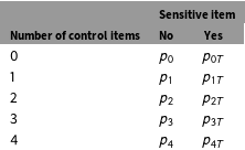
An important implication of no design effect and no liars is that researchers can recover—from the distribution of responses under control and treatment—the joint distribution of respondents’ preferences toward the sensitive item and the number of control items answered affirmatively (Glynn Reference Glynn2010). In particular, denote by
 $p_{k}$
the proportion of the population who respond affirmatively to
 $k$
control items and do not favor the sensitive item, and by
 $p_{kT}$
the proportion responding affirmatively to
 $k$
control items and favoring the sensitive item (shown in Table 1). Then
 $(p_{k},p_{kT})_{k=0}^{J}$
are identified under Assumptions 1 and 2.Footnote
3
Distribution of different types of respondents (
 $J=4$
).

2.2 No Liars Assumption
Ideally researchers would like all respondents to answer the list experiment question in a consistent and truthful way, satisfying the no design effect assumption and the no liars assumption. However, the no liars assumption is strong and may fail in many circumstances. For a treated respondent whose answer to all control items is affirmative and who favors the sensitive item, truth telling reveals with certainty that the respondent’s answer toward the sensitive item is affirmative, often referred to as ceiling effects in the literature (Kuklinski, Cobb, and Gilens Reference Kuklinski, Cobb and Gilens1997; Blair and Imai Reference Blair and Imai2012; Glynn Reference Glynn2013).Footnote 4 And for a treated respondent whose answer to a large number of control items is affirmative and who favors the sensitive item, intuitively, truth telling reveals with a high probability that the respondent’s answer toward the sensitive item is affirmative. Respondents who feel strongly about the social norm and fear their preferences for the sensitive item might be revealed thus have an incentive to lie about the sensitive item under list experiments, which leads to a violation of the no liars assumption. Moreover, failing to understand the protective nature of the list experiment design, actively managing perceptions about oneself (Köszegi Reference Köszegi2006) and being too embarrassed to admit also lead respondents to form untruthful latent response to the sensitive item.
Statistical tests are useful to detect certain violations of the assumptions, but there are limitations to these tests. Blair and Imai (Reference Blair and Imai2012) propose to test the positivity of the proportions of different types of respondents,
 $(p_{k},p_{kT})_{k=0}^{J}$
. However, they note that “the violation of Assumption 2 [no liars] alone does not lead to negative proportions of these types” and “researchers may fail to reject the null hypothesis due to a lack of statistical power” (Blair and Imai Reference Blair and Imai2012, pp. 64–65). In other words, the utility of the test is primarily detecting failures of the no design effect assumption and lack of statistical power can be a concern. Follow-up work by Aronow et al. (Reference Aronow, Coppock, Crawford and Green2015) proposes a complementary test when a direct question to the same respondents is also available.Footnote
5
Their test, however, can only detect violations of list experiment assumptions for respondents who reveal preferences for the sensitive item under the direct question.
In a recent validation study, Rosenfeld, Imai, and Shapiro (Reference Rosenfeld, Imai and Shapiro2016) find their list experiment underestimates sensitive votes against a referendum. One possible explanation for this observation is that some respondents give untruthful answers for the sensitive item.
In this paper, I will maintain the no design effect assumption and relax the no liars assumption. It will become clear that the no design effect assumption has important implications for identifying different types of respondents on its own and my analysis depends critically on it. For further discussion of this assumption, see Section A.6 in the supplementary materials.
2.3 Identification in the Absence of no Liars Assumption
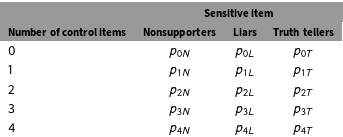
In the absence of the no liars assumption, the decomposition of respondent types in Table 1 is no longer valid. Instead, I denote the population fraction of respondents who answer affirmatively to
 $k$
control items and (1) do not favor the sensitive item by
 $p_{kN}$
; (2) favor the sensitive item, but would not give the truthful answer for it by
 $p_{kL}$
; (3) favor the sensitive item, and give the truthful answer for it by
 $p_{kT}$
. In particular, the proportion
 $p_{k}$
of respondents who answer in the affirmative to
 $k$
control items now consists of both the proportion
 $p_{kN}$
of nonsupporters and the proportion
 $p_{kL}$
of liars. Assuming only one side of the sensitive item is potentially socially undesirable, i.e.,
One-sided sensitivity assumption: Respondents who do not favor the sensitive item do not lie and falsely give an affirmative answer.
I can present the population distribution of different types of respondents in Table 2. In this terminology, the no liars assumption states that
 $p_{kL}=0$
for all
 $k$
.
Distribution of different types of respondents
 $(J=4)$
.

Researchers do not observe a respondent’s latent answer for the control items or the latent attitude toward the sensitive item (except when the respondent gives an answer of 0 or
 $J$
). What researchers observe is a response from 0 to
 $J$
for each respondent under the control condition, and a response from 0 to
 $J+1$
for each respondent under the treatment condition. Let
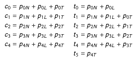
 $c_{k}$
be the population proportion of respondents whose answer is
 $k$
under the control condition and
 $t_{k}$
be the analogous proportion under the treatment condition, with
 $\sum _{k=0}^{J}c_{k}=\sum _{k=0}^{J+1}t_{k}=1$
.
To map a respondent’s latent response toward the control items and the latent attitude toward the sensitive item to his or her answer under the control condition, take a respondent who answers one item as an example. This respondent must answer affirmatively to exactly one control item, but I do not have any information about his or her attitude toward the sensitive item. The respondent may or may not favor the sensitive item, and in the latter case might or might not give a truthful answer for it if he or she were assigned to the treatment condition instead. Therefore, I have
 $c_{1}=p_{1N}+p_{1L}+p_{1T}$
. In the same fashion, I can express each
 $c_{k}$
in terms of the
 $p$
-terms, as shown in the left column in Table 3.
For a treated respondent, I can establish the mapping in a similar way. For example, to see
 $t_{1}=p_{1N}+p_{1L}+p_{0T}$
, notice that a response of one item under treatment comes from a respondent who (1) answers affirmatively to exactly one control item and does not favor the sensitive item, or (2) answers affirmatively to exactly one control item and favors the sensitive item, but does not give a truthful answer for it, or (3) answers affirmatively to no control items, but favors the sensitive item and is truthful. The expressions for all
 $t_{k}$
in terms of the
 $p$
-terms are shown in the right column in Table 3.
Relationship between latent attitudes and observable responses
 $(J=4)$
.

In Table 3, there are more unknown parameters than equations. Hence, the system of equations is underidentified and I cannot identify the distribution of all latent types,
 $(p_{kL},p_{kN},p_{kT})_{k=0}^{J}$
. A closer inspection reveals the reason why this system is underidentified. A lying respondent who actually favors the sensitive item is observationally equivalent to a respondent who does not favor the sensitive item at all, conditional on the same number of control items answered affirmatively. As a result, only the sum of the proportions of these two types is identified. In particular, regarding
 $p_{kN}+p_{kL}$
as one parameter instead of two parameters
 $p_{kN}$
and
 $p_{kL}$
, the system is exactly identified and I can identify
 $p_{kN}+p_{kL}$
and
 $p_{kT}$
for each
 $k=1,\ldots ,J$
.
2.4 Relaxed Liars Assumption, Bounds and Inference
The quantity of interest is the population proportion of respondents who favor the sensitive item,
 $\sum _{k=0}^{J}p_{kL}+p_{kT}$
. I have already shown that the proportion of truth tellers who respond affirmatively to
 $k$
control items,
 $p_{kT}$
, is identified for each
 $k$
, the remaining work concerns the fraction of respondents who favor the sensitive item but do not give truthful answers for it,
 $\sum _{k=0}^{J}p_{kL}$
. Since
 $p_{kN}+p_{kL}$
is identified for each
 $k=1,\ldots ,J$
, by setting all
 $p_{kL}$
’s to be zero (no liars), I obtain the standard difference-in-means estimator as a lower bound of the level of support for the sensitive item. At the other extreme, if I set all
 $p_{kN}$
’s to be zero (no nonsupporters), I obtain a trivial upper bound of 1.
With no behavioral assumption about the pattern of lying, I do not have an informative upper bound on the prevalence of the sensitive item. Toward a nontrivial upper bound, I propose the following assumption concerning the incentive to lie:
Relaxed liars assumption:
 $$\begin{eqnarray}\frac{p_{kL}}{p_{kL}+p_{kT}}\leqslant \frac{p_{JL}}{p_{JL}+p_{JT}},\quad \forall k=0,\ldots ,J-1,\end{eqnarray}$$
where
 $p_{kL}/(p_{kL}+p_{kT})$
is the ratio of liars conditional on responding affirmatively to
 $k$
control items and favoring the sensitive item. This assumption says that among all respondents who favor the sensitive item, the ones who respond affirmatively to all control items have the strongest incentive to lie. It relaxes the assumption of no liars, which amounts to
 $p_{kL}/(p_{kL}+p_{kT})\equiv 0$
for all
 $k=0,\ldots ,J$
. The relaxed liars assumption is simple and intuitive, and it captures the intuition behind the ceiling effect that truth telling reveals with certainty a respondent’s preference for the sensitive item when he or she favors all items. Also note that this assumption does not impose any relationship between lying incentives for respondents favoring fewer than all control items.
My relaxed liars assumption gives an upper bound for the number of liars among respondents who favor fewer than all control items. However, I need an estimate or upper bound on
 $p_{JL}$
to make this assumption implementable. Since
 $p_{JN}+p_{JL}$
is identified, it can serve as an upper bound. This bound will be crude unless
 $p_{JN}$
is relatively small. As presented in Section 3, in some applications, the crude bound can nevertheless be informative. In other list experiments, the bound can be wide, in which case the no liars assumption is important to nail down the prevalence of the sensitive item. Nonzero lower bound on
 $p_{kN}$
,
 $k=0,\ldots ,J$
, would improve upon the crude bounds, but would also necessarily involve additional information and/or assumptions. Formally, an upper/lower bound for the level of support for the sensitive item is given by the solution to the following linear system:
 $$\begin{eqnarray}\begin{array}{@{}l@{}}\displaystyle \max _{(p_{kL},p_{kN},p_{kT})_{k=0}^{J}}\left/\min _{(p_{kL},p_{kN},p_{kT})_{k=0}^{J}}\,\mathop{\sum }_{k=0}^{J}p_{kL}+p_{kT}\right.\\ \text{s.t.}~c_{0}=p_{0N}+p_{0L}+p_{0T},\ldots ,c_{J}=p_{JN}+p_{JL}+p_{JT}\\ \phantom{\text{s.t.}~}t_{0}=p_{0N}+p_{0L},\ldots ,t_{J}=p_{JN}+p_{JL}+p_{J-1,T},~t_{J+1}=p_{JT}\\ \phantom{\text{s.t.}~}p_{kL}/(p_{kL}+p_{kT})\leqslant (p_{JN}+p_{JL})/(p_{JN}+p_{JL}+p_{JT}),\quad \forall k=0,\ldots ,J-1.\end{array}\end{eqnarray}$$
I derive the bounds in steps in Section A.1 in the supplementary materials, and the lower and upper bounds are given by
 $$\begin{eqnarray}\left[\mathop{\sum }_{k=0}^{J}p_{kT},\mathop{\sum }_{k=0}^{J}p_{kT}+\mathop{\sum }_{k=0}^{J}\min \left\{\frac{\unicode[STIX]{x1D706}}{1-\unicode[STIX]{x1D706}}p_{kT},p_{kN}+p_{kL}\right\}\right]\end{eqnarray}$$
where
 $p_{kT}=\sum _{i=k+1}^{J+1}t_{i}-\sum _{j=k+1}^{J}c_{j}$
,
 $p_{kN}+p_{kL}=\sum _{j=k}^{J}c_{j}-\sum _{i=k+1}^{J+1}t_{i}$
, and the maximal liar ratio
 $\unicode[STIX]{x1D706}\equiv (p_{JN}+p_{JL})/(p_{JN}+p_{JL}+p_{JT})=(c_{J}-t_{J+1})/c_{J}$
. It follows that the bounds are nontrivial if and only if
 $\frac{\unicode[STIX]{x1D706}}{1-\unicode[STIX]{x1D706}}p_{kT}\leqslant p_{kN}+p_{kL}$
, or equivalently
 $p_{kT}/(p_{kN}+p_{kL})\leqslant p_{JT}/(p_{JN}+p_{JL})$
for some
 $k$
. In words, the condition holds if the proportion of truth-telling supporters is higher for respondents answering affirmatively to all
 $J$
control items than
 $k<J$
control items. A higher prevalence of the sensitive item will increase
 $\{p_{kT}\}_{k=0}^{J}$
but decrease
 $\unicode[STIX]{x1D706}$
, so the overall effect is ambiguous. Factors holding the prevalence fixed while decreasing the maximal liar ratio will narrow the bounds. I conduct detailed investigations in Section 3.
After identifying the lower and upper bounds, which I denote by
 $\hat{p}_{l}$
and
 $\hat{p}_{u}$
, I can construct the
 $(1-\unicode[STIX]{x1D6FC})$
-confidence intervals
 $\text{CI}(\hat{p}_{l})$
and
 $\text{CI}(\hat{p}_{u})$
via bootstrap. The confidence set formed by the lower endpoint of
 $\text{CI}(\hat{p}_{l})$
and the upper endpoint of
 $\text{CI}(\hat{p}_{u})$
covers the identified set with probability
 $(1-\unicode[STIX]{x1D6FC})$
, but will be slightly conservative in terms of covering the true prevalence of the sensitive item. Alternatively, I can construct the confidence set with
 $(1-\unicode[STIX]{x1D6FC})$
-coverage following Imbens and Manski (Reference Imbens and Manski2004) and Stoye (Reference Stoye2009) as
 $$\begin{eqnarray}\text{CI}_{\unicode[STIX]{x1D6FC}}=\left[\hat{p}_{l}-c_{\unicode[STIX]{x1D6FC}}\frac{\hat{\unicode[STIX]{x1D70E}}_{l}}{\sqrt{N}},\hat{p}_{u}+c_{\unicode[STIX]{x1D6FC}}\frac{\hat{\unicode[STIX]{x1D70E}}_{u}}{\sqrt{N}}\right],\end{eqnarray}$$
where
 $N$
is the total sample size,
 $\hat{\unicode[STIX]{x1D70E}}_{l}$
(
 $\hat{\unicode[STIX]{x1D70E}}_{u}$
) is the standard error for
 $\hat{p}_{l}$
(
 $\hat{p}_{u}$
), and
 $c_{\unicode[STIX]{x1D6FC}}$
solves
 $$\begin{eqnarray}\unicode[STIX]{x1D6F7}\left(c_{\unicode[STIX]{x1D6FC}}+\frac{\sqrt{N}}{\max \{\hat{\unicode[STIX]{x1D70E}}_{l},\hat{\unicode[STIX]{x1D70E}}_{u}\}}(\hat{p}_{u}-\hat{p}_{l})\right)-\unicode[STIX]{x1D6F7}(-c_{\unicode[STIX]{x1D6FC}})=1-\unicode[STIX]{x1D6FC},\end{eqnarray}$$
where
 $\unicode[STIX]{x1D6F7}$
is the standard normal cumulative distribution function.Footnote
6
,
Footnote
7
For a 95% confidence set,
 $c_{\unicode[STIX]{x1D6FC}}$
will be
 $\unicode[STIX]{x1D6F7}^{-1}(0.975)\approx 1.96$
if
 $\hat{p}_{u}-\hat{p}_{l}=0$
and will approach
 $\unicode[STIX]{x1D6F7}^{-1}(0.975)\approx 1.64$
as
 $\hat{p}_{u}-\hat{p}_{l}$
grows large relative to sampling error.
2.5 Extensions
2.5.1 Auxiliary Information to Sharpen Bounds
Further information can help us bound
 $p_{kN}$
and improve upon the crude upper bound. Auxiliary direct questions can be helpful to sharpen the bound. For example, researchers interested in learning the prevalence of anti-immigration attitudes can ask a direct question on support for a pathway to citizenship with possible choices yes, no, and ambivalent answers (not sure, rather not say, or do not know). The proportion of yes answers—indicating pro-immigration attitudes—among those who favor
 $k$
control items is a conservative estimate for
 $p_{kN}$
, under the assumption that the proportion of liars who answer yes to this direct question is smaller than that of nonsupporters who give negative or ambivalent answers.
2.5.2 Too Few Respondents on the Boundary
To reduce the number of respondents choosing zero or all items, some applied researchers include an item of very high prevalence and an item of very low prevalence. Glynn (Reference Glynn2013) instead suggests including negatively correlated items in favor of using high- or low-prevalence items. Both practices may result in very few respondents favoring all control items in some list experiments. In this case, the estimation of maximal liar ratio
 $(p_{JN}+p_{JL})/(p_{JN}+p_{JL}+p_{JT})$
in (2) relies on a small number of observations.
If answering affirmatively to all control items is vanishingly unlikely, then answering affirmatively to all but one control items is effectively an extreme response. So instead of estimating the maximal liar ratio as
 $(p_{JN}+p_{JL})/(p_{JN}+p_{JL}+p_{JT})$
in (2), I collapse the case of all control items and all but one control items and replace it with
 $(p_{J-1,N}+p_{J-1,L}+p_{JN}+p_{JL})/(p_{J-1,N}+p_{J-1,L}+p_{J-1,T}+p_{JN}+p_{JL}+p_{JT})$
, a quantity that can be more precisely estimated.Footnote
8
In words, I now require respondents favoring at least all but one control items to have stronger incentive to lie than those favoring fewer items.
3 Applications
3.1 Illustrative Example
For illustration, consider a list experiment Alvarez et al. (Reference Alvarez, Atkeson, Levin and Li2019) included in an online survey of 2,722 California adults conducted in 2014 using a sample recruited by Qualtrics. I excluded inattentive respondents who fail one of three trap questions included in the survey, and this leaves me with a total of 1,750 respondents.Footnote 9 The experiment was designed to measure the support for two state chapters of national anti-immigrant organizations among California residents. To preserve the anonymity of these organizations, I refer to them here as organization X and organization Y.
Respondents saw a control list or a treatment list with the names and short descriptions of different groups and organizations as shown in Table A.2, and were instructed to specify “how many of these groups and organizations you broadly support”.
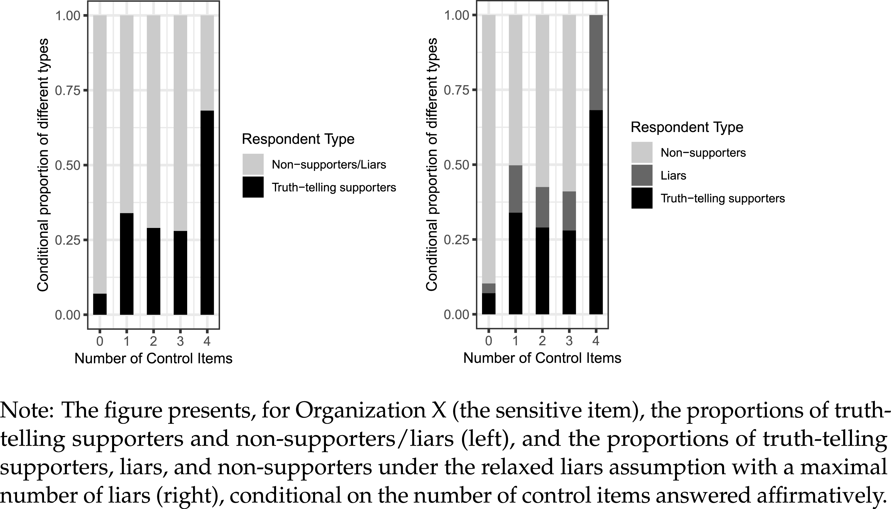
The proportions of control and treated respondents giving each answer are shown in Table A.3. Under the no design effect assumption, I can identify the proportions of truth-telling supporters and (truth-telling) nonsupporters/liars conditional on the number of control items answered affirmatively. Figure 1 shows these proportions for organization X on the left. If I further impose the relaxed liars assumption and allow a maximal number of liars, I can obtain the proportion of truth-telling supporters, the maximal proportion of liars, and the minimal proportion of nonsupporters, all conditional on the number of control items answered affirmatively. These proportions are shown in Figure 1 on the right.
Proportions of different types of respondents for Organization X.

Doing the calculations, the difference-in-means estimates are 0.36 for Organization X and 0.22 for Organization Y. 95% confident intervals for the point estimates are
 $[0.19,0.53]$
and
 $[0.05,0.39]$
, respectively. From my argument in Section 2, the difference-in-means estimate may understate the level of support for these organizations by neglecting respondents who support them but did not give truthful answers. If I allow the possibility of liars, but assume my relaxed liars assumption and implement my crude bound, I obtain an upper bound 0.53 for the level of support for Organization X, and 0.36 for Organization Y. 95% confidence sets for the interval estimates are
 $[0.23,0.80]$
and
 $[0.10,0.64]$
for Organization X and Organization Y, respectively. My bound estimates have important implications. To reach the conclusion that at most around a half respondents support Organization X and around a third respondents support Organization Y, I do not need to have full faith on the no liars assumption.
3.2 List Experiments in Published Studies
I now turn attention to a comprehensive set of list experiments in the political science literature, with basic information about these studies summarized in Table A.5.Footnote 10
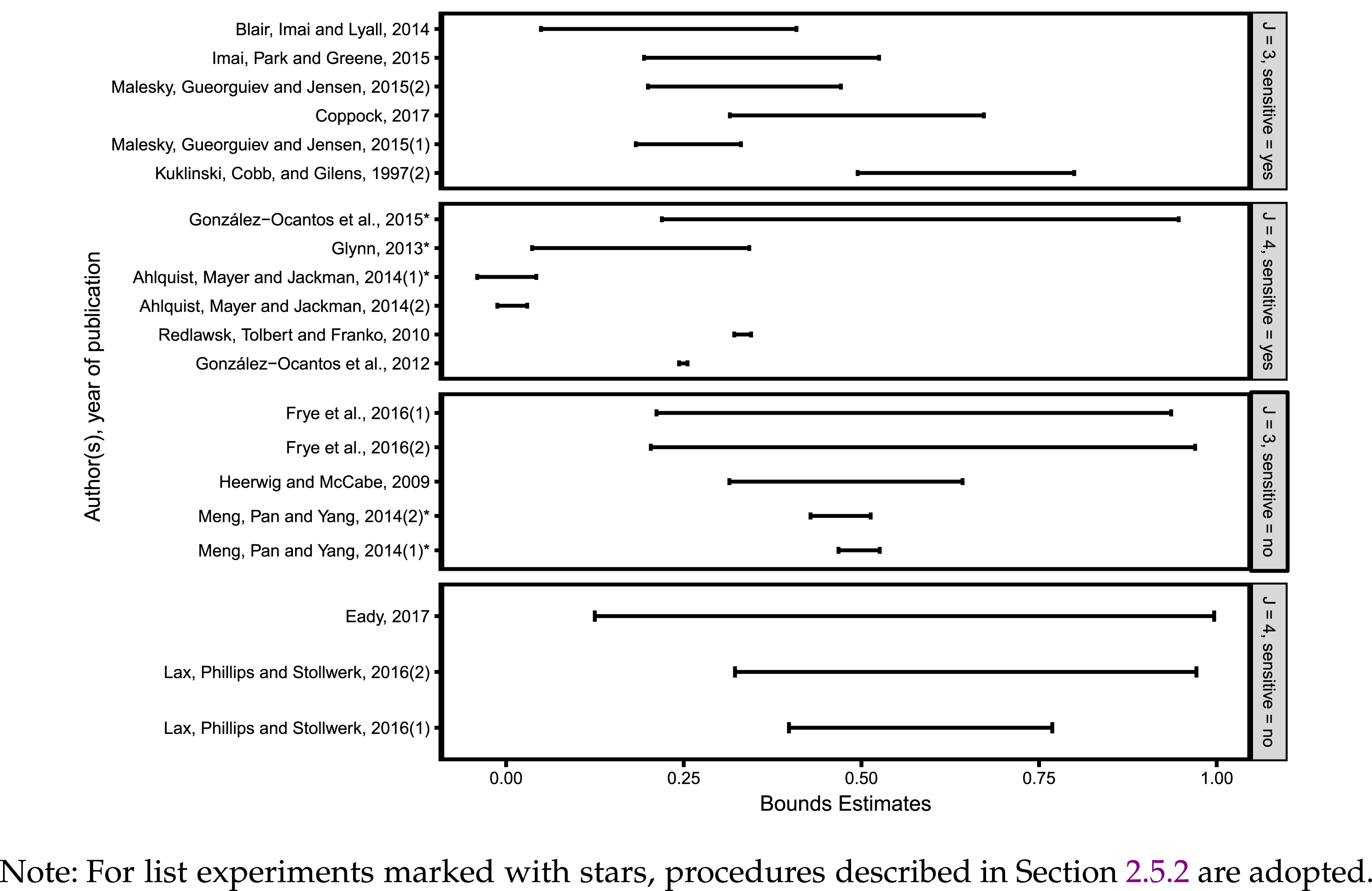
First notice that the list experiment concerning racial prejudice in Kuklinski, Cobb, and Gilens (Reference Kuklinski, Cobb and Gilens1997) and the list experiment concerning vote for an anti-abortion referendum in Rosenfeld, Imai, and Shapiro (Reference Rosenfeld, Imai and Shapiro2016) fail the Blair–Imai test of no design effect. Therefore, I exclude these applications from subsequent analysis. I now apply my method to obtain the range of the prevalence of sensitive behaviors or attitudes possible under the relaxed liars assumption for all other list experiments. Since no extra information for constructing tighter bounds for these studies is available, I compute my crude bounds. Recall that the lower bounds correspond to the difference-in-means estimates under the no liars assumption. In Figure 2, the intervals show the estimated lower and upper bounds.Footnote 11 The top two panels and the bottom two panels display studies with affirmative and negative sensitive responses, respectively. Within each panel, the studies are ordered by the maximal proportion of liars permitted by the relaxed liars assumption (with the largest value on the top).
Bound estimates for list experiments in published studies.

The widths of the intervals vary substantially across studies. Within each panel, the intervals tend to be narrower for studies with a smaller maximal proportion of liars permitted by the relaxed liars assumption. Across panels, the intervals appear to be narrower for list experiments with positive sensitive responses than those with negative sensitive responses, with the exception of Meng, Pan, and Yang (Reference Meng, Pan and Yang2014) and González-Ocantos, Kiewiet de Jonge, and Nickerson (Reference González-Ocantos, Kiewiet de Jonge and Nickerson2015). However, this pattern can be due to difference in other aspects of these list experiments; in fact, there is a symmetry between the case of an affirmative sensitive item and a negative sensitive item.Footnote 12 To better understand why some intervals are narrow and some are wide, I take a closer look at these list experiments.
As I showed in Section 2.3 and illustrated in the example, under no design effect, I can identify the proportions of (1) truth tellers with the sensitive behavior or attitude
 $p_{kT}$
, and (2) the combination of liars
 $p_{kL}$
and truth tellers without the sensitive behavior or attitude
 $p_{kN}$
, conditional on the number of control items answered affirmatively (or negatively for list experiments with negative sensitive responses). Figures A.1 and A.2 display these conditional proportions for studies with affirmative and negative sensitive responses, respectively. In other words, the lines in these figures correspond to the line connecting the top of the black bars shown in Figure 1. Since crude bounds use no external information about liars versus nonsupporters for sensitive items, narrower bounds come from: first, increasing proportions of truth tellers with the sensitive behavior/attitude conditional on the number of control items answered affirmatively/negatively, which corresponds to the inequalities in the relaxed liars assumption (1); second, a smaller maximal proportion of liars permitted by the relaxed liars assumption, which corresponds to the right hand side of (1). As shown in Figures A.1 and A.2, the increasing trend is present for many list experiments with affirmative sensitive responses and several with negative sensitive responses. This pattern explains why the intervals in Figure 2 appear to be narrower for these studies. Meanwhile, the widths of the intervals in Figure 2 are governed by the maximal possible proportion of liars in Figures A.1 and A.2, which in turn depends on the prevalence of different control and sensitive items that varies across studies.
One important implication is that the crude bound is more informative when the control items and the sensitive item are of the same type, which may give rise to positive correlation among different items. In a list experiment included in a large-scale administrative survey in Malesky, Gueorguiev, and Jensen (Reference Malesky, Gueorguiev and Jensen2015), items on the control and treatment lists are different activities that firms engage in to expedite the steps needed to receive their investment license/registration certificate. Another notable example is Meng, Pan, and Yang (Reference Meng, Pan and Yang2014), who study the factors that Chinese government officials consider when making local policy and expenditure decisions. Control items include considerations such as local administrative expenditures, influence in attracting foreign investment and scope of the migrant population, and the sensitive items are suggestions from residents expressed through formal state institutional channels and those through the Internet. Given the items included in these list experiments, it is not surprising that the crude bounds are informative, as is clear from Figure 2.
3.3 Simulated List Experiments
I now investigate the determinants of the length of the intervals through several simulated list experiments. The benefit of looking at these artificially generated list experiments is that I have full knowledge of the data generating processes, which is not the case for list experiments in published studies. I focus on the differences in the data generating processes and the resulting differences in the interval lengths, and not absolute lengths.
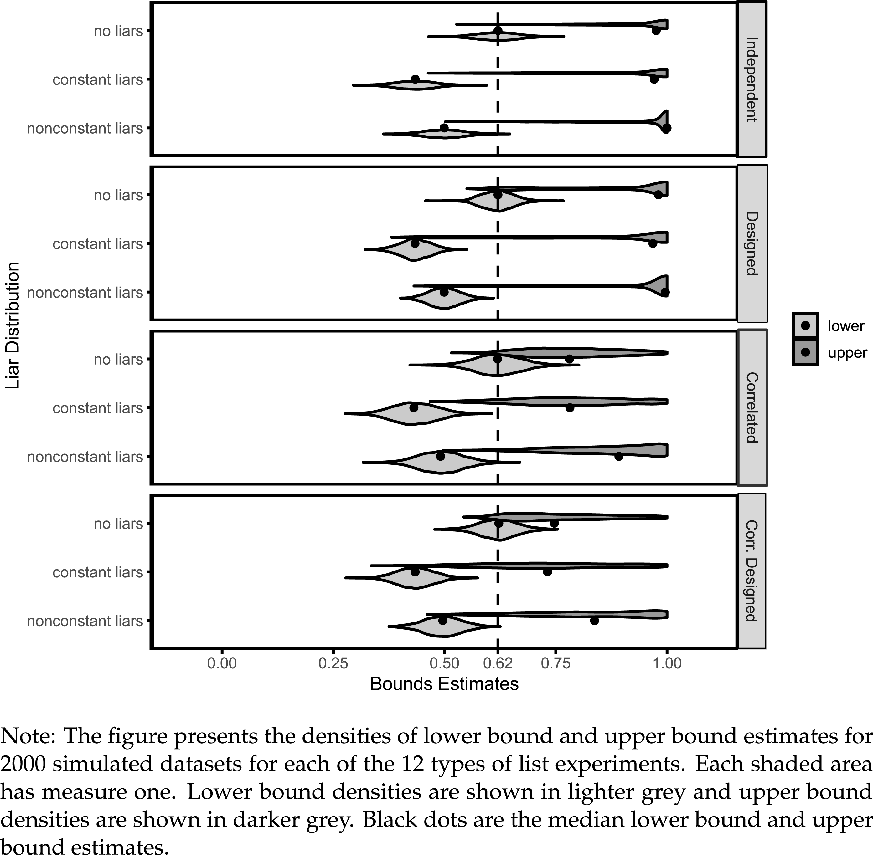
I consider a sensitive item of high prevalence (0.62) and list experiments of length 4 with 2,000 respondents in total, and vary the design of the control-item list and the distribution of liars conditional on the number of control items answered affirmatively.
I study four list structures. In an “independent” list, all control items are independent with prevalence
 $(1/6,1/2,2/3,2/3)$
, and independent from the sensitive item. In a “designed” list, there are high- and low-prevalence control items (0.85 and 0.15), as well as two negatively correlated control items, with prevalence 0.5 and correlation
 $-0.6$
. These parameter choices are borrowed from Ahlquist (Reference Ahlquist2017). I modify the “independent” lists and “designed” lists by adding 0.1 to the correlation of each pair of (control and sensitive) items, and refer to them as “correlated” and “correlated designed” lists.
I look at three different liar distributions. In the case of “no liars”, the lower bound—the difference-in-means estimate—consistently estimates the prevalence of the sensitive item. In the case of “constant liars”, I assume 30% of the respondents who favor the sensitive item answer the question as if they do not favor it. Finally, in the case of “nonconstant liars”, I assume
 $30\%\times 0.8^{k}$
liars for respondents who answer affirmatively to all but
 $k$
control items.
Bound estimates for simulated list experiments.

Figure 3 displays the densities and the medians of the crude bound estimates (lower bounds in lighter gray and upper bounds in darker gray) for 2,000 simulated datasets for each of the 12 types of list experiments under consideration. As expected, in the case of “no liars”, the lower bounds consistently estimate the prevalence of the sensitive item. In the case of “constant liars” and “nonconstant liars”, the lower bounds underestimate the prevalence of the sensitive item by the proportions of liars in the population, whereas the interval estimates cover the prevalence. If the sensitive item is truly independent of control items, then the prevalence of sensitive item conditional on the number of control items answered affirmatively is flat. And as the top half of the figure shows, I have trivial upper bounds most of the time for “independent” and “designed” lists. On the other hand, if there is positive correlation between the sensitive item and control items, then the prevalence of sensitive item conditional on the number of control items answered affirmatively is increasing. And as the bottom half of the figure shows, I have nontrivial upper bounds for “correlated” and “correlated designed” lists.
I present further simulations in the supplementary materials. The widths of the bounds are decreasing in the correlation between list items (Figures A.3 and A.4), consistent with our observation in Section 2.4 that decreasing the maximal liar ratio while keeping the prevalence fixed narrows the bounds. On the other hand, whether the sensitive response is affirmative or negative has no effect on the bound widths (Figure A.6), suggesting the differences between studies with affirmative and negative sensitive responses in Section 3.2 are due to differences in other aspects of these list experiments. Finally, list experiments with lower-prevalence items tend to produce slightly wider bounds in my simulations (Figure A.5).
3.4 Summary
By construction, the bounds will be nontrivial if and only if the proportion of truth-telling supporters is higher for respondents answering affirmatively to all
 $J$
control items than
 $k<J$
control items for some
 $k$
. The stronger the tendency that the proportion of truth-telling supporters increases in the number of control items answered affirmatively (especially when it approaches the boundary), the more informative the crude bounds are, as applications illustrate.
To put in primitive terms, the simulation exercise shows that positive correlation between the sensitive item and control items overall leads to narrower bounds, which is consistent with my previous observation that the width of the crude bound is narrower when items are of the same type. Absent such positive correlation, I expect uninformative bounds. For a list experiment with auxiliary question asking about the sensitive item directly, in addition to visualization in the form of Figure 1, researchers can also learn about the correlation by examining the correlation between control respondents’ answers to list experiment and their answers to the auxiliary question.Footnote 13
4 Discussion
4.1 Strengthening the Relaxed Liars Assumption
The relaxed liars assumption is a weaker assumption than the no liars assumption, leaving open the possibility that assumptions lying in between may give a tighter bound while accommodating the potential presence of liars. One such assumption states that the proportion of liars is increasing in the number of control items answered affirmatively:
 $$\begin{eqnarray}\frac{p_{kL}}{p_{kL}+p_{kT}}\leqslant \frac{p_{mL}}{p_{mL}+p_{mT}},\quad \forall 0\leqslant k<m\leqslant J-1.\end{eqnarray}$$
Without further information or assumption about the proportion of nonsupporters,
 $p_{mL}$
, one can weaken the inequality by replacing
 $p_{mL}/(p_{mL}+p_{mT})$
with
 $(p_{mL}+p_{mN})/(p_{mL}+p_{mN}+p_{mT})$
. Hence, the improvement of this stronger assumption over the relaxed liars assumption depends on the relationship between
 $(p_{mL}+p_{mN})/(p_{mL}+p_{mN}+p_{mT})$
and
 $(p_{JL}+p_{JN})/(p_{JL}+p_{JN}+p_{JT})$
. Since
 $(p_{JL}+p_{JN})/(p_{JL}+p_{JN}+p_{JT})$
—one minus the proportion of truth-telling supporters conditional on all control items answered affirmatively—is smaller for many list experiments in Section 3.2, the gain is limited for these applications.
4.2 Nonstrategic Respondent Error
By looking at violations of the no liars assumption, I essentially restrict attention to strategic misreporting. In addition to strategic misreporting, an inattentive respondent engaging in survey satisficing may choose randomly an answer, the first answer or the last answer from all options available, suggested by evidence from placebo list experiments (Holbrook and Krosnick Reference Holbrook and Krosnick2010; Ahlquist, Mayer, and Jackman Reference Ahlquist, Mayer and Jackman2014; Kiewiet de Jonge and Nickerson Reference Kiewiet de Jonge and Nickerson2014).Footnote 14 Alvarez et al. (Reference Alvarez, Atkeson, Levin and Li2019) find in two datasets with screener questions, difference-in-means estimates for respondents failing screener questions are significantly different from those for attentive respondents.Footnote 15
Nonstrategic respondent error can lead to violations of no design effect, no liars, and my relaxed liars assumption, result in bias to the difference-in-means estimator and maximum likelihood estimator à la Imai (Reference Imai2011) (Ahlquist Reference Ahlquist2017), and undermine the validity of the bounds developed in this paper. For online surveys, I recommend that applied researchers use screener questions—instructional manipulation checks (Oppenheimer, Meyvis, and Davidenko Reference Oppenheimer, Meyvis and Davidenko2009; Berinsky, Margolis, and Sances Reference Berinsky, Margolis and Sances2014) or conventional instructed-response items (Alvarez et al. Reference Alvarez, Atkeson, Levin and Li2019)—to identify inattentive respondents so as to minimize such biases whenever possible. For face-to-face or telephone surveys (where survey satisficing is arguably less serious), screener questions are infeasible and researchers may have to rely on response time or other indicators to identify inattentive respondents.
4.3 Heterogeneous Lying Patterns
Some subgroups of respondents may be more truthful than others. If a respondent characteristic is correlated with both the number of control items answered affirmatively and lying about the sensitive item, then depending on the lying pattern and the magnitude of such correlation, it could potentially violate the relaxed liars assumption. For example, suppose respondents with less education are less likely to realize when ceiling effects are occurring and are more truthful as a result. Then the relaxed liars assumption will be violated if they are disproportionately more likely to answer affirmatively to all control items, and the magnitude is large enough to offset the strategic incentive underlying the assumption. Researchers can check whether respondents answering affirmatively to all control items are very different in composition from other respondents, and make changes to the control items if possible (for example, after a pilot study). If there is still concern, researchers can apply the method to each demographic group separately (estimation precision will be lower).
5 Conclusion
Standard analysis of list experiments requires a strong assumption on respondents’ truthfulness toward sensitive issues, known as no liars. In this paper, I derive bounds for the prevalence of sensitive behaviors or attitudes under a weaker behavioral assumption and apply my method to an example on anti-immigration attitudes and a broad set of list experiments in the literature. The widths of the bounds vary substantially across studies. In some cases, especially when items on the list are of the same category, I can still reach substantive conclusions without putting full faith on the no liars assumption. In other cases, the full power of the no liars assumption is needed to pin down the prevalence of the sensitive behaviors or attitudes. I suggest that applied researchers compute the bounds as a guard against potential existence of liars in list experiments.
List experiments are designed to incentivize more truth telling from respondents than direct questions, but how successfully any particular application achieves it is not clear.Footnote 16 In particular, a small incremental support for the sensitive item over direct questions can mean either a small social desirability bias, or an unsuccessful inducement of truth telling. The method proposed in this paper is a first attempt to accommodate the presence of liars. The bounds exploit underlying strategic incentives and information in list experiments, but can be uninformative depending on applications. When there are resources, applied researchers can also employ other strategies such as the randomized response technique and compare estimates to gain confidence.
The method I propose is an addition to the list experiment toolbox and applicable to a large number of list experiments. But post-data-collection methods should not substitute or be prioritized over efforts to design good list experiments in the first place. Applied researchers should carefully construct the list items so that the question looks natural and the sensitive item stands out to a lesser extent, and follow other recommended practices discussed in Blair and Imai (Reference Blair and Imai2012) and Glynn (Reference Glynn2013). Meanwhile, when the list features a positive correlation between the sensitive item and control items overall, researchers can exploit this opportunity to estimate bounds robust to the presence of liars.
Supplementary material
For supplementary material accompanying this paper, please visit https://doi.org/10.1017/pan.2019.7.