1 Introduction
The upright annular (circular) tank belongs to the historically oldest reservoir shapes with analytical sloshing solutions. Standing wave patterns (natural sloshing modes) for the upright circular tank were first described by Ostrogradsky (Reference Ostrogradsky1832, submitted to the Paris Academy of Sciences in 1826) by introducing what we now name the Bessel functions. Analytical and experimental studies of the nonlinear resonant sloshing with longitudinal harmonic excitations started approximately 60 years ago. Interested readers can find more on these studies in the NASA Reports by Abramson (Reference Abramson1966) and Abramson, Chu & Kana (Reference Abramson, Chu and Kana1966a ) (see also references therein) as well as in the papers by Hutton (Reference Hutton1963, Reference Hutton1964), Abramson, Chu & Kana (Reference Abramson, Chu and Kana1966b ) and Chu (Reference Chu1968). A focus was on steady-state wave regimes. Modulated (nearly steady-state) resonant waves were examined by Miles (Reference Miles1984a ,Reference Miles b ). The resonant longitudinally excited sloshing in an upright circular tank was experimentally studied by Royon-Lebeaud, Hopfinger & Cartellier (Reference Royon-Lebeaud, Hopfinger and Cartellier2007) and Hopfinger & Baumbach (Reference Hopfinger and Baumbach2009) with an emphasis on the steady-state wave regimes, wave breaking and other free-surface phenomena. The multimodal analysis by Faltinsen, Rognebakke & Timokha (Reference Faltinsen, Rognebakke and Timokha2003) was used to qualitatively classify the observed steady-state resonant liquid motions.
The multimodal method is a powerful analytical tool for studying and simulating the nonlinear resonant sloshing. Its idea, technical details, advantages and drawbacks are described in Faltinsen & Timokha (Reference Faltinsen and Timokha2009, chaps. 7–9). Assuming an ideal incompressible liquid with irrotational flow and adopting a variational formulation, the method derives a (modal) system of nonlinear ordinary differential equations with respect to the generalised coordinates of the natural sloshing modes. When pursuing analytical studies, the system normally simplifies to a weakly nonlinear form by postulating asymptotic relations between these generalised coordinates. Reviews on the nonlinear modal systems for an upright circular (annular) reservoir can be found in Lukovsky (Reference Lukovsky1990, Reference Lukovsky2015), Lukovsky & Timokha (Reference Lukovsky and Timokha2011, Reference Lukovsky and Timokha2015) and Takahara & Kimura (Reference Takahara and Kimura2012). Adopting the Narimanov–Moiseev-type asymptotic relations is common. Examples are the five-dimensional modal system by Lukovsky (Reference Lukovsky1990, Reference Lukovsky2015) and the weakly nonlinear modal system by Takahara & Kimura (Reference Takahara and Kimura2012) who have in addition to Lukovsky’s approximation accounted for eight second- and third-order generalised coordinates. Since the Narimanov–Moiseev relations require the inclusion of, for axisymmetric tanks, two dominant lowest-order generalised coordinates (responsible for the two lowest degenerate antisymmetric natural sloshing modes) and an infinite number of both second- and third-order generalised coordinates, these weakly nonlinear modal systems are not complete from a mathematical point of view. The completeness suggests that the number of the second- and third-order generalised coordinates should not be fixed a priori but be a consequence of convergence analysis. Lukovsky, Ovchynnykov & Timokha (Reference Lukovsky, Ovchynnykov and Timokha2012) made an attempt to derive a complete modal system of the Narimanov–Moiseev-type for an upright circular tank but their paper contains a derivation error (see discussion in § 2.3).
The first goal of the present paper consists of deriving the complete weakly nonlinear Narimanov–Moiseev’s modal system for an upright annular/circular cylindrical tank. This is done in § 2 by using the analytical technique of Faltinsen & Timokha (Reference Faltinsen and Timokha2013). The derivations are verified by comparing the hydrodynamic coefficients of the system with those tabled by Lukovsky (Reference Lukovsky1990, Reference Lukovsky2015) for his five-dimensional modal approximation (§ 2.3). Adopting the Narimanov–Moiseev asymptotic relations assumes a small amplitude of excitation with the forcing frequency
 $\unicode[STIX]{x1D70E}$
close to the lowest natural sloshing frequency. The asymptotic relations also require no secondary (internal) resonances occurring when the
 $2\unicode[STIX]{x1D70E}$
or
 $3\unicode[STIX]{x1D70E}$
harmonics are close to a natural sloshing frequency of a second- or third-order mode/generalised coordinate, respectively (see an extensive discussion on the secondary resonance concept in chaps. 8 and 9 of Faltinsen & Timokha Reference Faltinsen and Timokha2009). Applicability of the derived modal system is investigated by evaluating the secondary resonance occurrence versus the liquid-depth-to-outer-cylinder-radius ratio
 $h$
and the central pole radius-to-outer-cylinder-radius ratio
 $r_{1}$
. In § 2.4, areas (zones) of
 $(h,r_{1})$
are specified where the system is applicable. This normally requires a fairly deep liquid depth,
 $1.5\lesssim h$
and
 $r_{1}$
should be away from 0.08546, 0.17618, 0.27826, 0.31323, 0.31855, 0.43444, 0.46015, 0.48434, 0.68655, 0.70118. Increasing the forcing amplitude increases the secondary resonance ranges around the aforementioned critical
 $r_{1}$
. The modal system can be used for modelling the experimental studies with the upright circular tank of Abramson et al. (Reference Abramson, Chu and Kana1966a
,Reference Abramson, Chu and Kana
b
) (
 $h=2$
) and Royon-Lebeaud et al. (Reference Royon-Lebeaud, Hopfinger and Cartellier2007) (
 $h=1.5$
) but experiments by Takahara & Kimura (Reference Takahara and Kimura2012) (an annular tank with
 $h=0.3$
and 1.0) generally need an adaptive asymptotic ordering, which makes it possible to adequately describe the secondary resonance effect.
The upright annular (or circular) tank shape is relevant for spacecraft applications (if the surface tension is accounted for, see p. 3 in Abramson Reference Abramson1966), it can be associated with a pressure-suppression pool of boiling water reactors (Aslam, Godden & Scalise Reference Aslam, Godden and Scalise1979), storage tanks (Balendra et al. Reference Balendra, Ang, Paramasivam and Lee1982; Tedesco, Landis & Kostem Reference Tedesco, Landis and Kostem1989) and tuned liquid dampers mitigating the vibration of wind turbines (Ghaemmaghami, Kianoush & Yuan Reference Ghaemmaghami, Kianoush and Yuan2013). Partly filled upright cylindrical shafts of offshore concrete towers (Chakrabarti Reference Chakrabarti1987; Faltinsen & Timokha Reference Faltinsen and Timokha2009), circular basins and annular flumes of aquacultural engineering (Pirhonen & Forsman Reference Pirhonen and Forsman1998; Timmons, Summerfelt & Vinci Reference Timmons, Summerfelt and Vinci1998; Fredriksson, Tsukrov & Hudson Reference Fredriksson, Tsukrov and Hudson2008) are other classes of applications. Resonant sloshing in upright circular/annular tanks has been studied for the longitudinal (horizontal and/or angular) harmonic forcing. Stable steady-state planar (in the excitation plane), swirling and irregular (unstable) waves were detected and described, experimentally and theoretically, for instance, in Abramson et al. (Reference Abramson, Chu and Kana1966a ,Reference Abramson, Chu and Kana b ), Lukovsky (Reference Lukovsky1990, Reference Lukovsky2015), Royon-Lebeaud et al. (Reference Royon-Lebeaud, Hopfinger and Cartellier2007), Faltinsen & Timokha (Reference Faltinsen and Timokha2009, chap. 9) and Takahara & Kimura (Reference Takahara and Kimura2012). A recent review on sloshing with parametric (vertical) excitations is given by Ibrahim (Reference Ibrahim2015).
The aforementioned industrial applications deal generally speaking with the coupled three-dimensional rigid-body dynamics. This causes a particular interest in analytical studies of resonant sloshing with a three-dimensional harmonic forcing. To the authors’ knowledge, the literature on that point is empty and there are no answers as to what kind of steady-state regimes are expected when the tank moves along a closed three-dimensional orbit. These (stable and unstable) regimes should differ from the longitudinally exited ones. Employing the derived modal system, we originate a pioneering study in this direction assuming a combined surge-sway-pitch-roll harmonic tank motion which, as we show, leads to either longitudinal or elliptic forcing (a formal definition of elliptic tank forcing is given in § 3). The purely elliptic and circular (rotary) type tank motions may appear for a combined pitch-and-roll (precession like) oscillation of missiles around the rocket mass centre. The reservoir can also move elliptically when it is suspended to a physical pendulum that is subject of the pendulum-slosh problem (Turner, Bridges & Ardakani Reference Turner, Bridges and Ardakani2015). The rotary forcing was used in the experiments by Prandtl (Reference Prandtl1949) and Faller (Reference Faller2001) to achieve a robust resonant steady-state rotary wave swirling with equivalent amplitudes in the two perpendicular horizontal directions. Their choice of the rotary forcing was not theoretically justified.
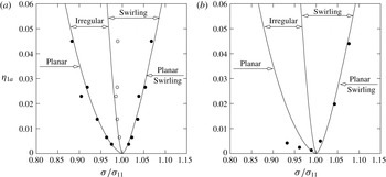
The second goal of the present paper consists, therefore, of studying the steady-state resonance sloshing with elliptic and rotary-type tank excitations. In § 3, we construct asymptotic periodic (steady-state) solutions of the derived nonlinear modal system and investigate their stability. A general elliptic harmonic forcing is assumed so that longitudinal and rotary excitations are particular cases of the proposed analytical asymptotic scheme. To validate the asymptotic solutions and the stability analysis, we focus in § 4 on the steady-state results for the longitudinal harmonic forcing. These theoretical results are validated by experimental observations and measurements of Abramson et al. (Reference Abramson, Chu and Kana1966a
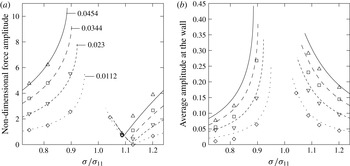
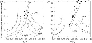
) and Royon-Lebeaud et al. (Reference Royon-Lebeaud, Hopfinger and Cartellier2007). Agreement is good for the effective frequency ranges where planar waves, swirling and irregular waves are realised. The horizontal hydrodynamic force caused by the planar waves is also well predicted. For the planar waves, the theoretical steady-state wave elevations at the vertical wall are in satisfactory agreement with the experimental measurements. The difference between the theory and the experiments for swirling may be affected by contributions from higher modes (see discussion in Faltinsen, Rognebakke & Timokha Reference Faltinsen, Rognebakke and Timokha2006), wave breaking and other complex free-surface phenomena which are observed and extensively described by Royon-Lebeaud et al. (Reference Royon-Lebeaud, Hopfinger and Cartellier2007). Modelling these phenomena needs a viscous hydrodynamic solution. The effect of the inner radius
 $r_{1}$
on the steady-state wave regimes with longitudinal forcing is analysed. We show that the
 $r_{1}$
-value influences the effective frequency ranges where stable planar, swirling and irregular (unstable) waves are expected. For
 $1.5\lesssim h$
, the stable swirling and/or irregular waves may disappear and only planar waves are stable for all resonance forcing frequencies when
 $r_{1}\approx 0.25$
and 0.35.
In § 5, we focus on the response curves for the elliptic forcing with
 $1.5\lesssim h$
and the admissible inner radius
 $r_{1}$
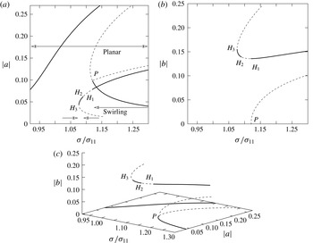
away from the aforementioned values 0.25 and 0.35. This forcing means that planar waves are impossible. We distinguish then the steady-state swirling waves propagating in two opposite angular directions. One wave is co-directed with the forcing but the other swirling wave is counter-directed. These two waves possess different amplitudes and stability properties. We draw the corresponding response curves for
 $h=2$
and
 $r_{1}=0$
, but the results remain qualitatively the same for
 $r_{1}$
away from 0.25 and 0.35. The branching versus the minor-to-major-axis component ratio of the elliptic forcing is studied. Increasing the ratio leads to vanishing irregular waves but the stable co-directed swirling wave tends to have equal amplitudes in the perpendicular horizontal directions, namely, the steady-state wave becomes close to rotary swirling. The aforementioned stable counter-directed (to the forcing) swirling wave also exists in a certain resonance frequency range. This range is almost independent of the minor-axis forcing component. The rotary swirling becomes the unique stable wave for the purely rotary (circular) forcing (see § 6); all other steady-state resonant waves become then unstable. The latter fact clarifies the advantages of using rotary forcing in studying the swirling-like free-surface phenomena as was done by Prandtl (Reference Prandtl1949) and Faller (Reference Faller2001).
2 Nonlinear modal equations
2.1 Fully nonlinear modal equations
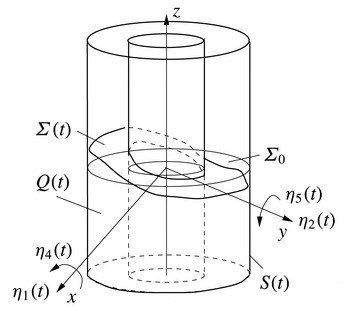
An inviscid incompressible contained liquid with irrotational flows is assumed. We consider liquid sloshing in an upright annular rigid tank with (outer) radius
 $\bar{r}_{2}$
performing small-magnitude sway, surge, roll and pitch motions (no heave and yaw) which are described by the
 $\bar{r}_{2}$
-scaled generalised coordinates
 $\unicode[STIX]{x1D702}_{1}(t)$
and
 $\unicode[STIX]{x1D702}_{2}(t)$
(responsible for translatory horizontal tank motions) and angular perturbations (generalised coordinates)
 $\unicode[STIX]{x1D702}_{4}(t)$
and
 $\unicode[STIX]{x1D702}_{5}(t)$
. The yaw tank motions cannot excite sloshing within the framework of the inviscid potential flow model. Heave (vertical) excitations are not considered. All geometric and physical parameters are henceforth considered scaled by
 $\bar{r}_{2}$
. We introduce a small parameter
 $\unicode[STIX]{x1D716}\ll 1$
characterising the forcing, i.e.
 $\unicode[STIX]{x1D702}_{i}(t)=O(\unicode[STIX]{x1D716}),i=1,2,4,5$
.
The time-dependent liquid domain
 $Q(t)$
confined by the free surface
 $\unicode[STIX]{x1D6F4}(t)$
and the wetted tank surface
 $S(t)$
. The free-surface evolution is considered in the tank-fixed coordinate system
 $Oxyz$
whose coordinate plane
 $Oxy$
coincides with the mean free surface
 $\unicode[STIX]{x1D6F4}_{0}$
and
 $Oz$
is the symmetry axis. Small-magnitude tank motions are governed by the generalised coordinates
 $\unicode[STIX]{x1D702}_{1}(t)$
(surge),
 $\unicode[STIX]{x1D702}_{4}(t)$
(roll),
 $\unicode[STIX]{x1D702}_{2}(t)$
(sway) and
 $\unicode[STIX]{x1D702}_{5}(t)$
(pitch).

The geometric notations are defined in figure 1 and include the time-dependent liquid domain
 $Q(t)$
with the free surface
 $\unicode[STIX]{x1D6F4}(t)$
and the wetted tank surface
 $S(t)$
. The free surface
 $\unicode[STIX]{x1D6F4}(t)$
is governed by the single-valued function
 $z=\unicode[STIX]{x1D701}(r,\unicode[STIX]{x1D703},t)$
and the liquid flow is determined by the velocity potential
 $\unicode[STIX]{x1D6F7}(r,\unicode[STIX]{x1D703},z,t)$
. The unknowns,
 $\unicode[STIX]{x1D701}$
and
 $\unicode[STIX]{x1D6F7}$
, are defined in the tank-fixed Cartesian (or equivalent cylindrical) coordinate system. The functions
 $\unicode[STIX]{x1D701}$
and
 $\unicode[STIX]{x1D6F7}$
can be found from either the corresponding free-surface problem or its equivalent variational formulation (see chap. 2 by Faltinsen & Timokha Reference Faltinsen and Timokha2009, and references therein).
The Bateman–Luke variational principle normally facilitates the multimodal method, which is based on the Fourier-type representations of
 $\unicode[STIX]{x1D701}$
and
 $\unicode[STIX]{x1D6F7}$
by the natural sloshing modes. The time-dependent coefficients in these Fourier representations are treated as independent time-varying generalised coordinates and velocities. The representations are normally based on the natural sloshing modes and frequencies given in an analytical form. The natural sloshing modes are the eigenfunctions of the spectral boundary problem
 $$\begin{eqnarray}\displaystyle \unicode[STIX]{x1D6FB}^{2}\unicode[STIX]{x1D711}=0\quad \text{in }Q_{0},\quad \frac{\unicode[STIX]{x2202}\unicode[STIX]{x1D711}}{\unicode[STIX]{x2202}n}=0\quad \text{on }S_{0e},S_{0i},S_{0b},\quad \frac{\unicode[STIX]{x2202}\unicode[STIX]{x1D711}}{\unicode[STIX]{x2202}n}=\unicode[STIX]{x1D705}\unicode[STIX]{x1D711}\quad \text{on }\unicode[STIX]{x1D6F4}_{0},\quad \int _{\unicode[STIX]{x1D6F4}_{0}}\unicode[STIX]{x1D711}\,\text{d}S=0 & & \displaystyle \nonumber\\ \displaystyle & & \displaystyle\end{eqnarray}$$
formulated in the mean liquid domain
 $Q_{0}$
confined by the mean free surface
 $\unicode[STIX]{x1D6F4}_{0}$
and the wetted tank surface
 $S_{0}$
(see notations in figure 2). The latter spectral boundary problem follows from the linear unforced sloshing problem of an inviscid incompressible liquid. The
 $\bar{r}_{2}$
-scaled spectral boundary problem (2.1) has the analytical solution (Faltinsen & Timokha Reference Faltinsen and Timokha2009; Lukovsky Reference Lukovsky2015)
 $$\begin{eqnarray}\displaystyle \unicode[STIX]{x1D711}_{Mi}(r,z,\unicode[STIX]{x1D703})=\mathscr{R}_{Mi}(r)\mathscr{Z}_{Mi}(z)_{\sin M\unicode[STIX]{x1D703}}^{\cos M\unicode[STIX]{x1D703}},\quad M=0,\ldots ;i=1,\ldots , & & \displaystyle\end{eqnarray}$$
where
 $$\begin{eqnarray}\displaystyle \mathscr{R}_{Mi}(r)=\unicode[STIX]{x1D6FC}_{Mi}\det \left|\text{}_{J_{M}^{\prime }(k_{Mi})}^{J_{M}(k_{Mi}r)}~\text{}_{Y_{M}^{\prime }(k_{Mi})}^{Y_{M}(k_{Mi}r)}\right|,\quad \mathscr{Z}_{Mi}(z)=\frac{\cosh (k_{Mi}(z+h))}{\cosh (k_{Mi}h)}. & & \displaystyle\end{eqnarray}$$
Here,
 $J_{M}(\cdot )$
and
 $Y_{M}(\cdot )$
are the Bessel functions of the first and second kinds, respectively. The radial wavenumbers
 $k_{Mi}$
are determined by
 $\mathscr{R}_{M,i}^{\prime }(r_{1})=0$
. The limit case
 $r_{1}=0$
(circular cylindrical tank) implies replacing (2.3) with
 $\mathscr{R}_{Mi}(r)=\unicode[STIX]{x1D6FC}_{Mi}J_{M}(k_{Mi}r)$
. The normalising multipliers
 $\unicode[STIX]{x1D6FC}_{Mi}$
follow from the orthogonality condition
 $$\begin{eqnarray}\displaystyle \unicode[STIX]{x1D706}_{(Mi)(Mj)}=\int _{r_{1}}^{1}r\mathscr{R}_{Mi}(r)\mathscr{R}_{Mj}(r)\,\text{d}r=\unicode[STIX]{x1D6FF}_{ij},\quad i,j=1,\ldots , & & \displaystyle\end{eqnarray}$$
where
 $\unicode[STIX]{x1D6FF}_{ij}$
is the Kronecker delta. The spectral parameter
 $\unicode[STIX]{x1D705}_{Mi}$
and the natural sloshing frequencies
 $\unicode[STIX]{x1D70E}_{Mi}$
are
 $$\begin{eqnarray}\displaystyle \unicode[STIX]{x1D705}_{Mi}=k_{Mi}\tanh (k_{Mi}h),\quad \unicode[STIX]{x1D70E}_{Mi}^{2}=\unicode[STIX]{x1D705}_{Mi}\bar{g}/\bar{r}_{2}=\unicode[STIX]{x1D705}_{Mi}g, & & \displaystyle\end{eqnarray}$$
where
 $\bar{g}$
is the gravitational acceleration.
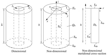
Dimensional and non-dimensional sketches of the mean liquid domain
 $Q_{0}$
in an upright annular tank. The non-dimensional mean liquid depth is
 $h$
, the inner radius equals to
 $r_{1}$
and the outer radius is equal to 1. The mean free surface is
 $\unicode[STIX]{x1D6F4}_{0}$
, the wetted inner and outer walls are
 $S_{0i}$
and
 $S_{0e}$
, respectively;
 $S_{0b}$
is the bottom. The corresponding boundaries in the meridional cross-section are denoted by the
 $L_{0\ast }$
symbols.

Dealing with small-amplitude angular tank excitations requires the linearised Stokes–Joukowski potentials
 $\unicode[STIX]{x1D6FA}_{0i}(r,z,\unicode[STIX]{x1D703}),i=1,2,3$
, which are harmonic functions satisfying the Neumann boundary conditions (Faltinsen & Timokha Reference Faltinsen and Timokha2009, § 5.4.4)
 $$\begin{eqnarray}\displaystyle \frac{\unicode[STIX]{x2202}\unicode[STIX]{x1D6FA}_{01}}{\unicode[STIX]{x2202}n}=-(zn_{r}-rn_{z})\sin \unicode[STIX]{x1D703},\quad \frac{\unicode[STIX]{x2202}\unicode[STIX]{x1D6FA}_{02}}{\unicode[STIX]{x2202}n}=(zn_{r}-rn_{z})\cos \unicode[STIX]{x1D703},\quad \frac{\unicode[STIX]{x2202}\unicode[STIX]{x1D6FA}_{03}}{\unicode[STIX]{x2202}n}=0 & & \displaystyle\end{eqnarray}$$
on
 $\unicode[STIX]{x1D6F4}_{0}$
,
 $S_{0i},S_{0e},$
and
 $S_{0b}$
(see notations in figure 2), where
 $n_{r}$
and
 $n_{z}$
are the outer normal components in the
 $r$
and
 $z$
directions so that
 $n_{z}=0$
on the vertical walls
 $L_{0i}$
and
 $L_{0e}$
but
 $n_{r}=0$
on
 $L_{0}$
and
 $L_{b}$
. This implies
 $\unicode[STIX]{x1D6FA}_{01}=-F(r,z)\sin \unicode[STIX]{x1D703}$
,
 $\unicode[STIX]{x1D6FA}_{02}=F(r,z)\cos \unicode[STIX]{x1D703}$
,
 $\unicode[STIX]{x1D6FA}_{03}=0$
, where
 $$\begin{eqnarray}\displaystyle F(r,z)=rz+\mathop{\sum }_{n=1}^{\infty }-\frac{2P_{n}}{k_{1n}}\mathscr{R}_{1n}(r)\frac{\sinh \left(k_{1n}\left(z+{\textstyle \frac{1}{2}}h\right)\right)}{\cosh \left({\textstyle \frac{1}{2}}k_{1n}h\right)},\quad P_{n}=\int _{r_{1}}^{1}r^{2}\mathscr{R}_{1n}(r)\,\text{d}r.\qquad & & \displaystyle\end{eqnarray}$$
Using the Bateman–Luke variational principle, Faltinsen & Timokha (Reference Faltinsen and Timokha2009) derived the fully nonlinear modal system with respect to the generalised coordinates (
 $p_{Mi}(t)$
and
 $r_{mi}(t)$
) and velocities (
 $P_{Mi}(t)$
and
 $R_{mi}(t)$
) in the Fourier (modal) solution
 $$\begin{eqnarray}\displaystyle \unicode[STIX]{x1D701}(r,\unicode[STIX]{x1D703},t)=\mathop{\sum }_{M,i}^{I_{\unicode[STIX]{x1D703}},I_{r}}\mathscr{R}_{Mi}(r)\cos (M\unicode[STIX]{x1D703})p_{Mi}(t)+\mathop{\sum }_{m,i}^{I_{\unicode[STIX]{x1D703}},I_{r}}\mathscr{R}_{mi}(r)\sin (m\unicode[STIX]{x1D703})r_{mi}(t), & & \displaystyle\end{eqnarray}$$
 $$\begin{eqnarray}\displaystyle \unicode[STIX]{x1D6F7}(r,\unicode[STIX]{x1D703},z,t) & = & \displaystyle \dot{\unicode[STIX]{x1D702}}_{1}(t)r\cos \unicode[STIX]{x1D703}+\dot{\unicode[STIX]{x1D702}}_{2}(t)r\sin \unicode[STIX]{x1D703}+F(r,z)[-\dot{\unicode[STIX]{x1D702}}_{4}(t)\sin \unicode[STIX]{x1D703}+\dot{\unicode[STIX]{x1D702}}_{5}(t)\cos \unicode[STIX]{x1D703}]\nonumber\\ \displaystyle & & \displaystyle +\,\mathop{\sum }_{M,i}^{I_{\unicode[STIX]{x1D703}},I_{r}}\mathscr{R}_{Mi}(r)\mathscr{Z}_{Mi}(z)\cos (M\unicode[STIX]{x1D703})P_{Mi}(t)+\mathop{\sum }_{m,i}^{I_{\unicode[STIX]{x1D703}},I_{r}}\mathscr{R}_{mi}(r)\mathscr{Z}_{mi}(z)\sin (m\unicode[STIX]{x1D703})R_{mi}(t),\nonumber\\ \displaystyle & & \displaystyle\end{eqnarray}$$
 $I_{\unicode[STIX]{x1D703}},I_{r}\rightarrow \infty$
. Here and further, all capital summation letters imply summing from zero to
 $I_{\unicode[STIX]{x1D703}}$
but the lower case indices mean changing from one to either
 $I_{\unicode[STIX]{x1D703}}$
or
 $I_{r}$
.
We assume a resonant sloshing when the hydrodynamic generalised coordinates
 $O(\unicode[STIX]{x1D716})\lesssim p_{Mi}(t),r_{mi}(t)$
and velocities
 $O(\unicode[STIX]{x1D716})\lesssim P_{Mi}(t),R_{mi}(t)$
are of a lower asymptotic order than
 $O(\unicode[STIX]{x1D716})$
. The
 $o(\unicode[STIX]{x1D716})$
-quantities associated with the nonlinear Stokes–Joukowski potential are omitted so that (2.8b
) only linearly depends on
 $\unicode[STIX]{x1D702}_{i}(t)$
as occurs in linear sloshing theory (see details in Faltinsen & Timokha Reference Faltinsen and Timokha2009, chaps. 5 and 7). The general fully nonlinear modal system can then be expressed as
 $$\begin{eqnarray}\displaystyle & \displaystyle \mathop{\sum }_{M,n}^{I_{\unicode[STIX]{x1D703}},I_{r}}\frac{\unicode[STIX]{x2202}A_{Ab}^{p}}{\unicode[STIX]{x2202}p_{Mn}}{\dot{p}}_{Mn}+\mathop{\sum }_{m,n}^{I_{\unicode[STIX]{x1D703}},I_{r}}\frac{\unicode[STIX]{x2202}A_{Ab}^{p}}{\unicode[STIX]{x2202}r_{mn}}{\dot{r}}_{mn}=\mathop{\sum }_{M,n}^{I_{\unicode[STIX]{x1D703}},I_{r}}A_{(Ab)(Mn)}^{pp}P_{Mn}+\mathop{\sum }_{m,n}^{I_{\unicode[STIX]{x1D703}},I_{r}}A_{(Ab),(Mn)}^{pr}R_{mn}, & \displaystyle\end{eqnarray}$$
 $$\begin{eqnarray}\displaystyle & \displaystyle \mathop{\sum }_{M,n}^{I_{\unicode[STIX]{x1D703}},I_{r}}\frac{\unicode[STIX]{x2202}A_{ab}^{r}}{\unicode[STIX]{x2202}p_{Mn}}{\dot{p}}_{Mn}+\mathop{\sum }_{m,n}^{I_{\unicode[STIX]{x1D703}},I_{r}}\frac{\unicode[STIX]{x2202}A_{ab}^{r}}{\unicode[STIX]{x2202}r_{mn}}{\dot{r}}_{mn}=\mathop{\sum }_{M,n}^{I_{\unicode[STIX]{x1D703}},I_{r}}A_{(Mn),(ab)}^{pr}P_{Mn}+\mathop{\sum }_{m,n}^{I_{\unicode[STIX]{x1D703}},I_{r}}A_{(ab)(mn)}^{rr}R_{mn}, & \displaystyle\end{eqnarray}$$
 $A=0,\ldots ,I_{\unicode[STIX]{x1D703}};a=1,\ldots ,I_{\unicode[STIX]{x1D703}};b=1,\ldots ,I_{r};I_{\unicode[STIX]{x1D703}},I_{r}\rightarrow \infty$
, the kinematic subsystem) and
 $$\begin{eqnarray}\displaystyle & & \displaystyle \displaystyle \mathop{\sum }_{M,n}^{I_{\unicode[STIX]{x1D703}},I_{r}}\frac{\unicode[STIX]{x2202}A_{Mn}^{p}}{\unicode[STIX]{x2202}p_{Ab}}{\dot{P}}_{Mn}+\mathop{\sum }_{m,n}^{I_{\unicode[STIX]{x1D703}},I_{r}}\frac{\unicode[STIX]{x2202}A_{mn}^{r}}{\unicode[STIX]{x2202}p_{Ab}}{\dot{R}}_{mn}+\frac{1}{2}\mathop{\sum }_{ML,nk}^{I_{\unicode[STIX]{x1D703}},I_{r}}\frac{\unicode[STIX]{x2202}A_{(Mn)(Lk)}^{pp}}{\unicode[STIX]{x2202}p_{Ab}}P_{Mn}P_{Lk}\nonumber\\ \displaystyle & & \displaystyle \displaystyle \quad +\,\mathop{\sum }_{Ml,nk}^{I_{\unicode[STIX]{x1D703}},I_{r}}\frac{\unicode[STIX]{x2202}A_{(Mn),(lk)}^{pr}}{\unicode[STIX]{x2202}p_{Ab}}P_{Mn}R_{lk}+\frac{1}{2}\mathop{\sum }_{ml,nk}^{I_{\unicode[STIX]{x1D703}},I_{r}}\frac{\unicode[STIX]{x2202}A_{(mn)(lk)}^{rr}}{\unicode[STIX]{x2202}P_{Ab}}R_{mn}R_{lk}+g\unicode[STIX]{x1D6EC}_{AA}p_{Ab}\nonumber\\ \displaystyle & & \displaystyle \displaystyle \quad +\,(\ddot{\unicode[STIX]{x1D702}}_{1}-g\unicode[STIX]{x1D702}_{5}-S_{b}\ddot{\unicode[STIX]{x1D702}}_{5})\unicode[STIX]{x1D6EC}_{1A}P_{b}=0,\end{eqnarray}$$
 $$\begin{eqnarray}\displaystyle & & \displaystyle \displaystyle \mathop{\sum }_{M,n}^{I_{\unicode[STIX]{x1D703}},I_{r}}\frac{\unicode[STIX]{x2202}A_{Mn}^{p}}{\unicode[STIX]{x2202}r_{ab}}{\dot{P}}_{Mn}+\mathop{\sum }_{m,n}^{I_{\unicode[STIX]{x1D703}},I_{r}}\frac{\unicode[STIX]{x2202}A_{mn}^{r}}{\unicode[STIX]{x2202}r_{ab}}{\dot{R}}_{mn}+\frac{1}{2}\mathop{\sum }_{ML,nk}^{I_{\unicode[STIX]{x1D703}},I_{r}}\frac{\unicode[STIX]{x2202}A_{(Mn)(Kl)}^{pp}}{\unicode[STIX]{x2202}r_{ab}}P_{Mn}P_{Lk}\nonumber\\ \displaystyle & & \displaystyle \displaystyle \quad +\,\mathop{\sum }_{Nl,nk}^{I_{\unicode[STIX]{x1D703}},I_{r}}\frac{\unicode[STIX]{x2202}A_{(Mn),(lk)}^{pr}}{\unicode[STIX]{x2202}r_{ab}}P_{Mn}R_{lk}+\frac{1}{2}\mathop{\sum }_{ml,nk}^{I_{\unicode[STIX]{x1D703}},I_{r}}\frac{\unicode[STIX]{x2202}A_{(mn)(lk)}^{rr}}{\unicode[STIX]{x2202}r_{ab}}R_{mn}R_{lk}+g\unicode[STIX]{x1D6EC}_{aa}r_{ab}\nonumber\\ \displaystyle & & \displaystyle \displaystyle \quad +\,(\ddot{\unicode[STIX]{x1D702}}_{2}+g\unicode[STIX]{x1D702}_{4}+S_{b}\ddot{\unicode[STIX]{x1D702}}_{4})\unicode[STIX]{x1D6EC}_{1a}P_{b}=0,A=0,\ldots ,I_{\unicode[STIX]{x1D703}};\quad a=1,\ldots ,I_{\unicode[STIX]{x1D703}};b=1,\ldots ,I_{r},\nonumber\\ \displaystyle & & \displaystyle\end{eqnarray}$$
 $I_{\unicode[STIX]{x1D703}},I_{r}\rightarrow \infty$
, where a comma between pairs of indices, such as
 $(Ab),(Mn)$
, means that the pairs do not commutate; coefficients
 $P_{b}$
are defined in (2.7),
 $$\begin{eqnarray}\displaystyle S_{b}=2k_{1b}^{-1}\tanh \left(k_{1b}\frac{h}{2}\right),\quad \unicode[STIX]{x1D6EC}_{IJ}=\left\{\begin{array}{@{}ll@{}}2\unicode[STIX]{x03C0},\quad & I=J=0,\\ \unicode[STIX]{x03C0}\unicode[STIX]{x1D6FF}_{IJ},\quad & \text{otherwise},\end{array}\right. & & \displaystyle\end{eqnarray}$$
where
 $\unicode[STIX]{x1D6FF}_{IJ}$
is the Kronecker delta. Faltinsen & Timokha (Reference Faltinsen and Timokha2013) wrote down this system for a spherical tank which differs from (2.9) and (2.10) by the forcing terms whose expressions for the annular (circular) tanks can be found in Ch. 5 of Faltinsen & Timokha (Reference Faltinsen and Timokha2009).
The modal system (2.9), (2.10) contains the following nonlinear functions of the hydrodynamic generalised coordinates
 $$\begin{eqnarray}\displaystyle \left.\begin{array}{@{}c@{}}\displaystyle A_{(Ab)(Mn)}^{pp}=\int _{r_{1}}^{1}\int _{-\unicode[STIX]{x03C0}}^{\unicode[STIX]{x03C0}}r[\cos A\unicode[STIX]{x1D703}\cos M\unicode[STIX]{x1D703}\mathscr{G}_{(Ab)(Mn)}^{(1)}+\sin A\unicode[STIX]{x1D703}\sin M\unicode[STIX]{x1D703}\mathscr{G}_{(Ab)(Mn)}^{(2)}]\,\text{d}\unicode[STIX]{x1D703}\,\text{d}r,\\ \displaystyle A_{(ab)(mn)}^{rr}=\int _{r_{1}}^{1}\int _{-\unicode[STIX]{x03C0}}^{\unicode[STIX]{x03C0}}r[\sin a\unicode[STIX]{x1D703}\sin m\unicode[STIX]{x1D703}\mathscr{G}_{(ab)(mn)}^{(1)}+\cos a\unicode[STIX]{x1D703}\cos m\unicode[STIX]{x1D703}\mathscr{G}_{(ab)(mn)}^{(2)}]\,\text{d}\unicode[STIX]{x1D703}\,\text{d}r,\\ \displaystyle A_{(Ab),(mn)}^{pr}=\int _{r_{1}}^{1}\int _{-\unicode[STIX]{x03C0}}^{\unicode[STIX]{x03C0}}r[\cos A\unicode[STIX]{x1D703}\sin m\unicode[STIX]{x1D703}\mathscr{G}_{(Ab)(mn)}^{(1)}-\sin A\unicode[STIX]{x1D703}\cos m\unicode[STIX]{x1D703}\mathscr{G}_{(Ab)(mn)}^{(2)}]\,\text{d}\unicode[STIX]{x1D703}\,\text{d}r,\\ \displaystyle A_{Ab}^{p}=\int _{r_{1}}^{1}\int _{-\unicode[STIX]{x03C0}}^{\unicode[STIX]{x03C0}}r\cos (A\unicode[STIX]{x1D703})\mathscr{G}_{Ab}^{(0)}\,\text{d}\unicode[STIX]{x1D703}\,\text{d}r,\quad A_{ab}^{r}=\int _{r_{1}}^{1}\int _{-\unicode[STIX]{x03C0}}^{\unicode[STIX]{x03C0}}r\sin (a\unicode[STIX]{x1D703})\mathscr{G}_{Ab}^{(0)}\,\text{d}\unicode[STIX]{x1D703}\,\text{d}r,\end{array}\right\}\qquad & & \displaystyle\end{eqnarray}$$
where
 $$\begin{eqnarray}\displaystyle \left.\begin{array}{@{}c@{}}\displaystyle \mathscr{G}_{Ab}^{(0)}=\mathscr{R}_{Ab}(r)\int _{-h}^{\unicode[STIX]{x1D701}}\frac{\cosh (k_{Ab}(z+h))}{\cosh (k_{Ab}h)}\,\text{d}z=\mathscr{R}_{Ab}(r)I_{(Ab)}^{(0)},\\ \displaystyle \mathscr{G}_{(Ab)(Mn)}^{(1)}=\mathscr{R}_{Ab}^{\prime }(r)\mathscr{R}_{Mn}^{\prime }(r)I_{(Ab)(Mn)}^{(1)}+\mathscr{R}_{Ab}(r)\mathscr{R}_{Mn}(r)k_{Ab}k_{Mn}I_{(Ab)(Mn)}^{(2)},\\ \displaystyle \mathscr{G}_{(Ab)(Mn)}^{(2)}=AMr^{-2}\mathscr{R}_{Ab}(r)\mathscr{R}_{Mn}(r)I_{(Ab)(Mn)}^{(1)};\end{array}\right\} & & \displaystyle\end{eqnarray}$$
 $$\begin{eqnarray}\displaystyle \left.\begin{array}{@{}c@{}}\displaystyle I_{(Ab)(Mn)}^{(1)}=\int _{-h}^{\unicode[STIX]{x1D701}}\frac{\cosh (k_{Ab}(z+h))\cosh (k_{Mn}(z+h))}{\cosh (k_{Ab}h)\cosh (k_{Mnh})}\,\text{d}z,\\ \displaystyle I_{(Ab)(Mn)}^{(2)}=\int _{-h}^{\unicode[STIX]{x1D701}}\frac{\sinh (k_{Ab}(z+h))\sinh (k_{Mn}(z+h))}{\cosh (k_{Ab}h)\cosh (k_{Mnh})}\,\text{d}z.\end{array}\right\} & & \displaystyle\end{eqnarray}$$
2.2 The Narimanov–Moiseev-type modal equations
Moiseev (Reference Moiseev1958) proposed an analytical scheme for constructing the periodic (steady-state) solution of the original free-surface sloshing problem by introducing
 $O(\unicode[STIX]{x1D716})$
-order harmonic excitation and so-called Moiseev detuning
 $$\begin{eqnarray}\displaystyle \bar{\unicode[STIX]{x1D70E}}_{11}^{2}-1=O(\unicode[STIX]{x1D716}^{2/3}),\quad \bar{\unicode[STIX]{x1D70E}}_{11}=\unicode[STIX]{x1D70E}_{11}/\unicode[STIX]{x1D70E}. & & \displaystyle\end{eqnarray}$$
The scheme implicitly assumes that there are no secondary resonances and other small non-dimensional parameters, e.g. shallow liquid depth. Moiseev’s analysis implies that the dominant steady-state sloshing response is of order
 $O(\unicode[STIX]{x1D716}^{1/3})$
and is contributed to solely by the primary excited modes.
Independently, Narimanov (Reference Narimanov1957) proposed an asymptotic scheme to derive a weakly nonlinear modal system assuming that the forcing is not necessarily periodic and is of order
 $O(\unicode[STIX]{x1D716})\ll 1$
. The latter means that the steady-state condition was relaxed and, therefore, the detuning condition (2.15) is not required. Narimanov’s scheme suggests that the primary excited generalised coordinates have the dominant character
 $O(\unicode[STIX]{x1D716}^{1/3})$
but the ordering of other generalised coordinates follows from the asymptotic scheme. Trigonometrical algebra by the angular coordinate
 $\unicode[STIX]{x1D703}$
shows that the axisymmetric tanks cause the following asymptotic relations for the generalised coordinates in the modal solution (2.8a
)
 $$\begin{eqnarray}\displaystyle \left.\begin{array}{@{}c@{}}\displaystyle p_{11}\sim r_{11}=O(\unicode[STIX]{x1D716}^{1/3}),\quad p_{0j}\sim p_{2j}\sim r_{2j}=O(\unicode[STIX]{x1D716}^{2/3}),\\ \displaystyle r_{1(j+1)}\sim p_{1(j+1)}\sim p_{3j}\sim r_{3j}=O(\unicode[STIX]{x1D716}),\quad j=1,2,\ldots ,I_{r};\quad I_{r}\rightarrow \infty .\end{array}\right\}\qquad & & \displaystyle\end{eqnarray}$$
The remaining generalised coordinates
 $r_{kl}\sim p_{kl}=o(\unicode[STIX]{x1D716}),k\geqslant 4$
and, therefore, these can be neglected. When adopting the periodicity condition and (2.15), one can show that Narimanov’s asymptotic scheme is equivalent to Moiseev’s derivations and leads to the same steady-state solution.
The asymptotic relations (2.16) mean that
 $I_{\unicode[STIX]{x1D703}}=3$
in (2.8). Using these relations and neglecting the
 $o(\unicode[STIX]{x1D716})$
terms (tedious but straightforward derivations are available in the supplementary materials at http://dx.doi.org/10.1017/jfm.2016.539) leads to the following Narimanov–Moiseev-type modal system
 $$\begin{eqnarray}\displaystyle & & \displaystyle \displaystyle \ddot{p}_{11}+\unicode[STIX]{x1D70E}_{11}^{2}p_{11}+d_{1}p_{11}(\ddot{p}_{11}p_{11}+\ddot{r}_{11}r_{11}+{\dot{p}}_{11}^{2}+{\dot{r}}_{11}^{2})\nonumber\\ \displaystyle & & \displaystyle \displaystyle \quad +\,d_{2}[r_{11}(\ddot{p}_{11}r_{11}-\ddot{r}_{11}p_{11})+2{\dot{r}}_{11}({\dot{p}}_{11}r_{11}-{\dot{r}}_{11}p_{11})]\nonumber\\ \displaystyle & & \displaystyle \displaystyle \quad +\,\mathop{\sum }_{j=1}^{I_{r}} [\!d_{3}^{(j)}(\ddot{p}_{11}p_{2j}+\ddot{r}_{11}r_{2j}+{\dot{p}}_{11}{\dot{p}}_{2j}+{\dot{r}}_{11}{\dot{r}}_{2j})+d_{4}^{(j)}(\ddot{p}_{2j}p_{11}+\ddot{r}_{2j}r_{11})\nonumber\\ \displaystyle & & \displaystyle \displaystyle \quad +\,d_{5}^{(j)}(\ddot{p}_{11}p_{0j}+{\dot{p}}_{11}{\dot{p}}_{0j})+d_{6}^{(j)}\ddot{p}_{0j}p_{11}\! ]=-(\ddot{\unicode[STIX]{x1D702}}_{1}-g\unicode[STIX]{x1D702}_{5}-S_{1}\ddot{\unicode[STIX]{x1D702}}_{5})\unicode[STIX]{x1D705}_{11}P_{1},\end{eqnarray}$$
 $$\begin{eqnarray}\displaystyle & & \displaystyle \displaystyle \ddot{r}_{11}+\unicode[STIX]{x1D70E}_{11}^{2}r_{11}+d_{1}r_{11}(\ddot{p}_{11}p_{11}+\ddot{r}_{11}r_{11}+{\dot{p}}_{11}^{2}+{\dot{r}}_{11}^{2})\nonumber\\ \displaystyle & & \displaystyle \quad \displaystyle +\,d_{2}[p_{11}(\ddot{r}_{11}p_{11}-\ddot{p}_{11}r_{11})+2{\dot{p}}_{11}({\dot{r}}_{11}p_{11}-{\dot{p}}_{11}r_{11})]\nonumber\\ \displaystyle & & \displaystyle \quad +\,\displaystyle \mathop{\sum }_{j=1}^{I_{r}} [\!d_{3}^{(j)}(\ddot{p}_{11}r_{2j}-\ddot{r}_{11}p_{2j}+{\dot{p}}_{11}{\dot{r}}_{2j}-{\dot{p}}_{2j}{\dot{r}}_{11})+d_{4}^{(j)}(\ddot{r}_{2j}p_{11}-\ddot{p}_{2j}r_{11})\nonumber\\ \displaystyle & & \displaystyle \displaystyle \quad +\,d_{5}^{(j)}(\ddot{r}_{11}p_{0j}+{\dot{r}}_{11}{\dot{p}}_{0j})+d_{6}^{(j)}\ddot{p}_{0j}r_{11}\! ]=-(\ddot{\unicode[STIX]{x1D702}}_{2}+g\unicode[STIX]{x1D702}_{4}+S_{1}\ddot{\unicode[STIX]{x1D702}}_{4})\unicode[STIX]{x1D705}_{11}P_{1};\end{eqnarray}$$
 $$\begin{eqnarray}\displaystyle & \displaystyle \ddot{p}_{2k}+\unicode[STIX]{x1D70E}_{2k}^{2}p_{2k}+d_{7,k}({\dot{p}}_{11}^{2}-{\dot{r}}_{11}^{2})+d_{9,k}(\ddot{p}_{11}p_{11}-\ddot{r}_{11}r_{11})=0, & \displaystyle\end{eqnarray}$$
 $$\begin{eqnarray}\displaystyle & \displaystyle \ddot{r}_{2k}+\unicode[STIX]{x1D70E}_{2k}^{2}r_{2k}+2d_{7,k}{\dot{p}}_{11}{\dot{r}}_{11}+d_{9,k}(\ddot{p}_{11}r_{11}+\ddot{r}_{11}p_{11})=0, & \displaystyle\end{eqnarray}$$
 $$\begin{eqnarray}\displaystyle & \displaystyle \ddot{p}_{0k}+\unicode[STIX]{x1D70E}_{0k}^{2}p_{0k}+d_{8,k}({\dot{p}}_{11}^{2}+{\dot{r}}_{11}^{2})+d_{10,k}(\ddot{p}_{11}p_{11}+\ddot{r}_{11}r_{11})=0; & \displaystyle\end{eqnarray}$$
 $$\begin{eqnarray}\displaystyle & & \displaystyle \displaystyle \ddot{p}_{3k}+\unicode[STIX]{x1D70E}_{3k}^{2}p_{3k}+d_{11,k}[\ddot{p}_{11}(p_{11}^{2}-r_{11}^{2})-2p_{11}r_{11}\ddot{r}_{11}]+d_{12,k}[p_{11}({\dot{p}}_{11}^{2}-{\dot{r}}_{11}^{2})-2r_{11}{\dot{p}}_{11}{\dot{r}}_{11}]\nonumber\\ \displaystyle & & \displaystyle \displaystyle \quad +\,\mathop{\sum }_{j=1}^{I_{r}} [\!d_{13,k}^{(j)}(\ddot{p}_{11}p_{2j}-\ddot{r}_{11}r_{2j})+d_{14,k}^{(j)}(\ddot{p}_{2j}p_{11}-\ddot{r}_{2j}r_{11})\nonumber\\ \displaystyle & & \displaystyle \displaystyle \quad +\,d_{15,k}^{(j)}({\dot{p}}_{2j}{\dot{p}}_{11}-{\dot{r}}_{2j}{\dot{r}}_{11})\!]=0,\end{eqnarray}$$
 $$\begin{eqnarray}\displaystyle & & \displaystyle \displaystyle \ddot{r}_{3k}+\unicode[STIX]{x1D70E}_{3k}^{2}r_{3k}+d_{11,k}[\ddot{r}_{11}(p_{11}^{2}-r_{11}^{2})+2p_{11}r_{11}\ddot{p}_{11}]+d_{12,k}[r_{11}({\dot{p}}_{11}^{2}-{\dot{r}}_{11}^{2})+2p_{11}{\dot{p}}_{11}{\dot{r}}_{11}]\nonumber\\ \displaystyle & & \displaystyle \displaystyle \quad +\,\mathop{\sum }_{j=1}^{I_{r}} [\!d_{13,k}^{(j)}(\ddot{p}_{11}r_{2j}+\ddot{r}_{11}p_{2j})+d_{14,k}^{(j)}(\ddot{p}_{2j}r_{11}+\ddot{r}_{2j}p_{11})\nonumber\\ \displaystyle & & \displaystyle \displaystyle +\,d_{15,k}^{(j)}({\dot{p}}_{2j}{\dot{r}}_{11}+{\dot{r}}_{2j}{\dot{p}}_{11})\!]=0,\quad k=1,\ldots ,I_{r};\end{eqnarray}$$
 $$\begin{eqnarray}\displaystyle & & \displaystyle \ddot{p}_{1n}+\unicode[STIX]{x1D70E}_{1n}^{2}p_{1n}+d_{16,n}(\ddot{p}_{11}p_{11}^{2}+r_{11}p_{11}\ddot{r}_{11})+d_{17,n}(\ddot{p}_{11}r_{11}^{2}-r_{11}p_{11}\ddot{r}_{11})+d_{18,n}p_{11}({\dot{p}}_{11}^{2}+{\dot{r}}_{11}^{2})\nonumber\\ \displaystyle & & \displaystyle \displaystyle \qquad +\,d_{19,n}(r_{11}{\dot{p}}_{11}{\dot{r}}_{11}-p_{11}{\dot{r}}_{11}^{2})+\mathop{\sum }_{j=1}^{I_{r}} [\!d_{20,n}^{(j)}(\ddot{p}_{11}p_{2j}+\ddot{r}_{11}r_{2j})+d_{21,n}^{(j)}(p_{11}\ddot{p}_{2j}+r_{11}\ddot{r}_{2j})\nonumber\\ \displaystyle & & \displaystyle \displaystyle \qquad +\,d_{22,n}^{(j)}({\dot{p}}_{11}{\dot{p}}_{2j}+{\dot{r}}_{11}{\dot{r}}_{2j})+d_{23,n}^{(j)}\ddot{p}_{11}p_{0j}+d_{24,n}^{(j)}p_{11}\ddot{p}_{0j}+d_{25,n}^{(j)}{\dot{p}}_{11}{\dot{p}}_{0j}\! ]\nonumber\\ \displaystyle & & \displaystyle \displaystyle \quad =-(\ddot{\unicode[STIX]{x1D702}}_{1}-g\unicode[STIX]{x1D702}_{5}-S_{n}\ddot{\unicode[STIX]{x1D702}}_{5})\unicode[STIX]{x1D705}_{1n}P_{n},\end{eqnarray}$$
 $$\begin{eqnarray}\displaystyle & & \displaystyle \displaystyle \ddot{r}_{1n}+\unicode[STIX]{x1D70E}_{1n}^{2}r_{1n}+d_{16,n}(\ddot{r}_{11}r_{11}^{2}+r_{11}p_{11}\ddot{p}_{11})+d_{17,n}(\ddot{r}_{11}p_{11}^{2}-r_{11}p_{11}\ddot{p}_{11})+d_{18,n}r_{11}({\dot{p}}_{11}^{2}+{\dot{r}}_{11}^{2})\nonumber\\ \displaystyle & & \displaystyle \displaystyle \qquad +\,d_{19,n}(p_{11}{\dot{p}}_{11}{\dot{r}}_{11}-r_{11}{\dot{p}}_{11}^{2})+\mathop{\sum }_{j=1}^{I_{r}} [\!d_{20,n}^{(j)}(\ddot{p}_{11}r_{2j}-\ddot{r}_{11}p_{2j})+d_{21,n}^{(j)}(p_{11}\ddot{r}_{2j}-r_{11}\ddot{p}_{2j})\nonumber\\ \displaystyle & & \displaystyle \displaystyle \qquad +\,d_{22,n}^{(j)}({\dot{p}}_{11}{\dot{r}}_{2j}-{\dot{r}}_{11}{\dot{p}}_{2j})+d_{23,n}^{(j)}\ddot{r}_{11}p_{0j}+d_{24,n}^{(j)}r_{11}\ddot{p}_{0j}+d_{25,n}^{(j)}{\dot{r}}_{11}{\dot{p}}_{0j}\! ]\nonumber\\ \displaystyle & & \displaystyle \displaystyle \quad =-(\ddot{\unicode[STIX]{x1D702}}_{2}+g\unicode[STIX]{x1D702}_{4}+S_{n}\ddot{\unicode[STIX]{x1D702}}_{4})\unicode[STIX]{x1D705}_{1n}P_{n},\quad n=2,\ldots ,I_{r},\end{eqnarray}$$
 $I_{r}\rightarrow \infty$
. The system needs either an initial or periodicity condition that determines transient and steady-state solutions, respectively. Linear damping terms accounting for the viscous boundary layer and bulk damping can be incorporated as described in Ch. 6 of Faltinsen & Timokha (Reference Faltinsen and Timokha2009). The steady-state analysis of the modal system can be directly done by a numerical method but the present study does it in an analytical way.
When neglecting the nonlinear quantities, the modal system transforms to the linear modal equations (see chap. 5 of Faltinsen & Timokha Reference Faltinsen and Timokha2009) where only equations with indices
 $(1n),n\geqslant 1$
((2.17) and (2.20)) contain inhomogeneous terms and, therefore, imply forced sloshing. The two equations in (2.17) govern the dominant generalised coordinates
 $p_{11}$
and
 $r_{11}$
which depend on the second-order generalised coordinates determined from (2.18). Differential equations (2.19) and (2.20) are linear with respect to the third-order generalised coordinates and these coordinates do not appear in other differential equations. This means that the third-order hydrodynamic generalised coordinates are ‘driven’ by the lower-order ones. One can consider, as an exception, the case
 $I_{\unicode[STIX]{x1D703}}=2$
which means neglecting (2.19) and (2.20) with respect to the driven natural sloshing modes (generalised coordinates). The positive integer
 $I_{r}$
determines the number of differential equations in (2.18)–(2.20) as well as the summation limits in formulas for the hydrodynamic coefficients and the differential equations (2.17), (2.19) and (2.20).
The horizontal hydrodynamic forces can be expressed via the hydrodynamic generalised coordinates by using the Lukovsky formulas ((7.22) in Faltinsen & Timokha Reference Faltinsen and Timokha2009). The expressions are linear in
 $p_{1k},r_{1k},k=1,\ldots ,I_{r}$
and take the form
 $$\begin{eqnarray}\displaystyle \left.\begin{array}{@{}c@{}}\displaystyle F_{1}(t)=\unicode[STIX]{x03C0}\unicode[STIX]{x1D70C}\bar{r}_{2}^{4}\left[(1-r_{1}^{2})h\left(g\unicode[STIX]{x1D702}_{5}-\ddot{\unicode[STIX]{x1D702}}_{1}+\frac{1}{2}h\ddot{\unicode[STIX]{x1D702}}_{5}\right)-\mathop{\sum }_{j=1}^{I_{r}}P_{j}\ddot{p}_{1j}\right],\\ \displaystyle F_{2}(t)=\unicode[STIX]{x03C0}\unicode[STIX]{x1D70C}\bar{r}_{2}^{4}\left[(1-r_{1}^{2})h\left(-g\unicode[STIX]{x1D702}_{4}-\ddot{\unicode[STIX]{x1D702}}_{2}+\frac{1}{2}h\ddot{\unicode[STIX]{x1D702}}_{4}\right)-\mathop{\sum }_{j=1}^{I_{r}}P_{j}\ddot{r}_{1j}\right],\end{array}\right\} & & \displaystyle\end{eqnarray}$$
where the square bracket terms are scaled by
 $\bar{r}_{2}$
and
 $\unicode[STIX]{x1D70C}$
is the liquid density. Analogous Lukovsky’s formulas exist for the hydrodynamic moments (see chap. 7 of Faltinsen & Timokha Reference Faltinsen and Timokha2009).
2.3 Verification of (2.17) and (2.18)
The hydrodynamic coefficients can be compared with computations by other authors. Takahara & Kimura (Reference Takahara and Kimura2012) do not report the corresponding numerical values but Lukovsky (Reference Lukovsky1990, Reference Lukovsky2015) has tabled the hydrodynamic coefficients for a broad set of
 $r_{1}$
and
 $h$
. Lukovsky (Reference Lukovsky1990) derived the Narimanov–Moiseev modal equations adopting the following five-term approximate modal solution
 $$\begin{eqnarray}\displaystyle \unicode[STIX]{x1D701}(r,z,\unicode[STIX]{x1D703}) & = & \displaystyle \frac{\mathscr{R}_{01}(r)}{\mathscr{R}_{0}}p_{0}(t)+\frac{\mathscr{R}_{11}(r)}{\mathscr{R}_{1}}[p_{1}(t)\cos \unicode[STIX]{x1D703}+r_{1}(t)\sin \unicode[STIX]{x1D703}]\nonumber\\ \displaystyle & & \displaystyle +\,\frac{\mathscr{R}_{21}(r)}{\mathscr{R}_{2}}[p_{2}(t)\cos 2\unicode[STIX]{x1D703}+r_{2}(t)\sin 2\unicode[STIX]{x1D703}],\quad \mathscr{R}_{i}=\mathscr{R}_{i1}(1),i=0,1,2,\qquad\end{eqnarray}$$
which links the generalised coordinates (2.22) and (2.8a
) via the equality
 $p_{i}(t)=\mathscr{R}_{i}p_{i1}(t).$
The five-term approximation completely neglects the third-order modes contributions as well as excluding the second-order generalised coordinates with the indices
 $(0n),(2n),~n\geqslant 2$
. The authors’ experience with modal system for a rectangular cross-section shows that neglecting the third-order terms causes a less accurate quantitative prediction of the resonance response.
The five-dimensional modal system by Lukovsky (Reference Lukovsky2015, (4.1.15)–(4.1.19)) reads as
 $$\begin{eqnarray}\displaystyle & & \displaystyle \displaystyle \unicode[STIX]{x1D707}_{1}(\ddot{r}_{1}+\unicode[STIX]{x1D70E}_{1}^{2}r_{1})+d_{1}(r_{1}^{2}\ddot{r}_{1}+r_{1}{\dot{r}}_{1}^{2}+r_{1}p_{1}\ddot{p}_{1}+r_{1}{\dot{p}}_{1}^{2})+d_{2} (\!p_{1}^{2}\ddot{r}_{1}+2p_{1}{\dot{r}}_{1}{\dot{p}}_{1}\nonumber\\ \displaystyle & & \displaystyle \displaystyle \quad -\,r_{1}p_{1}\ddot{p}_{1}-2r_{1}{\dot{p}}_{1}^{2}\! )-d_{3}(r_{2}\ddot{r}_{1}-r_{2}\ddot{p}_{1}+{\dot{r}}_{1}{\dot{p}}_{2}-{\dot{p}}_{1}{\dot{r}}_{2})+d_{4}(r_{1}\ddot{p}_{2}-p_{1}\ddot{r}_{2})\nonumber\\ \displaystyle & & \displaystyle \displaystyle \quad +\,d_{5}(p_{0}\ddot{r}_{1}+{\dot{r}}_{1}{\dot{p}}_{0})+d_{6}r_{1}\ddot{p}_{0}=-P\ddot{\unicode[STIX]{x1D702}}_{2}(t),\end{eqnarray}$$
 $$\begin{eqnarray}\displaystyle & & \displaystyle \displaystyle \unicode[STIX]{x1D707}_{1}(\ddot{p}_{1}+\unicode[STIX]{x1D70E}_{1}^{2}p_{1})+d_{1}(p_{1}^{2}\ddot{p}_{1}+r_{1}p_{1}\ddot{r}_{1}+p_{1}{\dot{r}}_{1}^{2}+p_{1}{\dot{p}}_{1}^{2})+d_{2} (\!r_{1}^{2}\ddot{p}_{1}-r_{1}p_{1}\ddot{r}_{1}\nonumber\\ \displaystyle & & \displaystyle \displaystyle \quad +\,2r_{1}{\dot{r}}_{1}{\dot{p}}_{1}-2p_{1}{\dot{r}}_{1}^{2}\! )+d_{3}(p_{2}\ddot{p}_{1}+r_{2}\ddot{r}_{1}+{\dot{r}}_{1}{\dot{r}}_{2}+{\dot{p}}_{1}{\dot{p}}_{2})-d_{4}(p_{1}\ddot{p}_{2}+r_{1}\ddot{r}_{2})\nonumber\\ \displaystyle & & \displaystyle \displaystyle \quad +\,d_{5}(p_{0}\ddot{p}_{1}+{\dot{p}}_{1}{\dot{p}}_{0})+d_{6}p_{1}\ddot{p}_{0}=-P\ddot{\unicode[STIX]{x1D702}}_{1}(t),\end{eqnarray}$$
 $$\begin{eqnarray}\displaystyle \unicode[STIX]{x1D707}_{0}(\ddot{p}_{0}+\unicode[STIX]{x1D70E}_{0}^{2}p_{0})+d_{6}(r_{1}\ddot{r}_{1}+p_{1}\ddot{p}_{1})+d_{8}({\dot{r}}_{1}^{2}+{\dot{p}}_{1}^{2})=0, & & \displaystyle\end{eqnarray}$$
 $$\begin{eqnarray}\displaystyle \unicode[STIX]{x1D707}_{2}(\ddot{r}_{2}+\unicode[STIX]{x1D70E}_{2}^{2}r_{2})-d_{4}(p_{1}\ddot{r}_{1}+r_{1}\ddot{p}_{1})-2d_{7}{\dot{r}}_{1}{\dot{p}}_{1}=0, & & \displaystyle\end{eqnarray}$$
 $$\begin{eqnarray}\displaystyle \unicode[STIX]{x1D707}_{2}(\ddot{p}_{2}+\unicode[STIX]{x1D70E}_{2}^{2}p_{2})+d_{4}(r_{1}\ddot{r}_{1}-p_{1}\ddot{p}_{1})+d_{7}({\dot{r}}_{1}^{2}-{\dot{p}}_{1}^{2})=0. & & \displaystyle\end{eqnarray}$$
This means that
 $$\begin{eqnarray}\displaystyle \left.\begin{array}{@{}c@{}}\displaystyle d_{1}=\frac{d_{1}\mathscr{R}_{1}^{2}}{\unicode[STIX]{x1D707}_{1}},\quad d_{2}=\frac{d_{2}\mathscr{R}_{1}^{2}}{\unicode[STIX]{x1D707}_{1}},\quad d_{3}^{(1)}=\frac{d_{3}\mathscr{R}_{2}}{\unicode[STIX]{x1D707}_{1}},\quad d_{4}^{(1)}=-\frac{d_{4}\mathscr{R}_{2}}{\unicode[STIX]{x1D707}_{1}},\quad d_{5}^{(1)}=\frac{d_{5}\mathscr{R}_{0}}{\unicode[STIX]{x1D707}_{1}},\\ \displaystyle d_{6}^{(1)}=\frac{d_{6}\mathscr{R}_{0}}{\unicode[STIX]{x1D707}_{1}},\quad d_{7,1}=-\frac{d_{7}\mathscr{R}_{1}^{2}}{\mathscr{R}_{2}\unicode[STIX]{x1D707}_{2}},\quad d_{8,1}=\frac{d_{8}\mathscr{R}_{1}^{2}}{\mathscr{R}_{0}\unicode[STIX]{x1D707}_{0}},\\ \displaystyle d_{9,1}=-\frac{d_{4}\mathscr{R}_{1}^{2}}{\mathscr{R}_{2}\unicode[STIX]{x1D707}_{2}},\quad d_{10,1}=\frac{d_{6}\mathscr{R}_{1}^{2}}{\mathscr{R}_{0}\unicode[STIX]{x1D707}_{0}}.\end{array}\right\}\qquad & & \displaystyle\end{eqnarray}$$
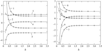
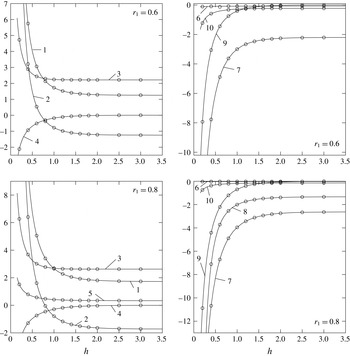
Values of hydrodynamic coefficients (vertical axes) of the Narimanov–Moiseev modal system within the framework of Lukovsky (Reference Lukovsky1990, Reference Lukovsky2015)’s five-dimensional approximation (
 $I_{\unicode[STIX]{x1D703}}=2,I_{r}=1$
in our computational formulas) versus the non-dimensional liquid depth
 $h$
. There is no inner pole,
 $r_{1}=0$
. The solid lines denote our calculations and the circles correspond to the tabled values from Lukovsky (Reference Lukovsky1990, Reference Lukovsky2015) rescaled according to (2.24). The integers on the graphs imply: 1 –
 $d_{1}$
, 2 –
 $d_{2}$
, 3 –
 $d_{3}^{(1)}$
, 4 –
 $d_{4}^{(1)}$
, 5 –
 $d_{5}^{(1)}$
, 6 –
 $d_{6}^{(1)}$
, 7 –
 $d_{7,1}$
, 8 –
 $d_{8,1}$
, 9 –
 $d_{9,1}$
, and 10 –
 $d_{10,1}$
.

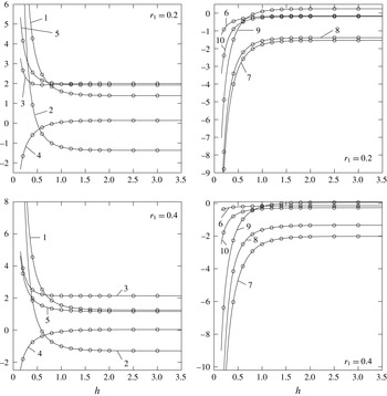
The same as in figure 3 but for annular cross-sections with
 $r_{1}=0.2$
and 0.4.

The same as in figure 3 but for annular cross-sections with
 $r_{1}=0.6$
and 0.8.

Computed hydrodynamic coefficients
 $d_{1}$
and
 $d_{2}$
for
 $h=1$
versus
 $I_{r}$
.
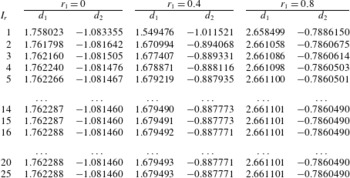
Our computations with
 $I_{\unicode[STIX]{x1D703}}=2$
and
 $I_{r}=1$
and the tabled hydrodynamic coefficients by Lukovsky (Reference Lukovsky1990, Reference Lukovsky2015) (rescaled by (2.24)) have a small relative difference which is less than 0.1 % that is actually the stated precision (from three to five digits) of Lukovsky’s computations. This fact is illustrated in figures 3–5. Increasing
 $I_{r}\geqslant 2$
increases the number of ordinary differential (modal) equations and may change the hydrodynamic coefficients at the cubic terms by the lowest-order generalised coordinates. These hydrodynamic coefficients,
 $d_{1},d_{2},d_{11,k},d_{12,k},d_{16,k}$
and
 $d_{18,k}$
, are functions of the upper summation limit
 $I_{r}$
. This means, in particular, that
 $d_{1}$
and
 $d_{2}$
in (2.23) cannot be used in Narimanov–Moiseev modal systems with
 $I_{r}\geqslant 2$
.
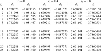
The numerical values of
 $d_{1}$
and
 $d_{2}$
versus
 $I_{r}$
are shown in table 1 for
 $h=1$
. The computations demonstrate that increasing
 $I_{r}$
may affect the coefficient values; the difference is not negligible for
 $r_{1}=0.4$
. Lukovsky et al. (Reference Lukovsky, Ovchynnykov and Timokha2012) missed out the dependence
 $d_{1}$
and
 $d_{2}$
on
 $I_{r}$
by taking
 $I_{r}=1$
in the corresponding formulas.
2.4 Applicability of the modal system (2.17)–(2.20)
The nonlinear modal theory (2.17)–(2.20) assumes that the forcing amplitude is sufficiently small and the forcing frequency
 $\unicode[STIX]{x1D70E}$
is close to the lowest natural sloshing frequency
 $\unicode[STIX]{x1D70E}_{11}$
. Another limitation is that the theory requires no secondary resonances (see the text below, § 2.2 as well as chaps. 8 and 9 of Faltinsen & Timokha Reference Faltinsen and Timokha2009, and references therein). Miles (Reference Miles1984b
) and Bryant (Reference Bryant1989) were, most probably, the first two scientists who paid attention to the secondary resonances for sloshing in upright circular cylindrical tanks. Nowadays, taking care of the secondary resonances is a necessary component of analytical and numerical studies. However, these studies mainly focus on prismatic tanks (see e.g. Ikeda, Harata & Osasa Reference Ikeda, Harata and Osasa2016, and references therein). We could only recall Gavrilyuk et al. (Reference Gavrilyuk, Lukovsky, Trotsenko and Timokha2007) and Takahara & Kimura (Reference Takahara and Kimura2012), where the secondary resonances were estimated for circular and annular upright containers, and Lukovsky & Timokha (Reference Lukovsky and Timokha2011) and Faltinsen & Timokha (Reference Faltinsen and Timokha2013), who discussed these resonances for sloshing in axisymmetric tanks.
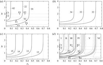
The curves specify the critical pairs of
 $r_{1}$
and
 $h$
where secondary resonance is possible. They are marked by the double indices
 $Mi$
of
 $p_{Mi}(t)$
and
 $r_{Mi}(t)$
, which are resonantly amplified owing to the second- (
 $M=0,2$
, panel (a), (2.25a
)) and third- (
 $M=3,1$
, panels (b) and (c), (2.25b
)) order secondary resonances. The case
 $r_{1}=0$
corresponds to the circular cross-section but the vertical asymptotes at a certain
 $r_{1}$
mean secondary resonance at infinite depth. The panel (d) summarises (a–c) and indicates the
 $(r_{1},h)$
zones (I–VI) where the modal system is applicable. The zones reduce with increasing of the forcing amplitude. The experimental cases by Abramson et al. (Reference Abramson, Chu and Kana1966a
,
 $\,h=2,r_{1}=0$
), Royon-Lebeaud et al. (Reference Royon-Lebeaud, Hopfinger and Cartellier2007,
 $\,h=1.5,r_{1}=0$
) and Takahara & Kimura (Reference Takahara and Kimura2012,
 $\,h=1,r_{1}=0.196,0.393;h=0.3,r_{1}=0.196,393$
) are marked by points C1, C2 and T1–T4, respectively. The cases E1 (
 $r_{1}=0.25$
) and E2 (
 $r_{1}=0.35$
) are discussed in § 4 in the context of
 $r_{1}$
for which the only planar steady-state regime becomes stable owing to longitudinal excitations.

Trigonometrical algebra by the angular coordinate
 $\unicode[STIX]{x1D703}$
determines the analytical structure of (2.18)–(2.20) where the dominant (lowest-order) generalised coordinates
 $p_{11}$
and
 $r_{11}$
(and their time derivatives) constitute quadratic terms in the modal equations with respect to
 $p_{2k},r_{2k}$
and
 $p_{0k}$
(here, in (2.18)) but the cubic quantities in
 $p_{11}$
and
 $r_{11}$
appear in (2.17) and (2.19)–(2.20). When the (mean) forcing frequency
 $\unicode[STIX]{x1D70E}$
is close to the lowest natural sloshing frequency
 $\unicode[STIX]{x1D70E}_{11}$
, the generalised coordinates
 $p_{11}$
and
 $r_{11}$
contain the resonantly excited harmonics
 $\cos \unicode[STIX]{x1D70E}t$
and
 $\sin \unicode[STIX]{x1D70E}t$
and the quadratic terms by
 $p_{11}$
and
 $r_{11}$
in (2.18) yield the
 $2\unicode[STIX]{x1D70E}$
harmonics. If the double harmonics are close to one of the natural sloshing frequencies
 $\{\unicode[STIX]{x1D70E}_{2k},\unicode[STIX]{x1D70E}_{0k}\}$
, a resonant amplification of the corresponding second-order generalised coordinate occurs. Analogously, cubic quantities in (2.19)–(2.20) yield the
 $3\unicode[STIX]{x1D70E}$
harmonics which can be close to
 $\unicode[STIX]{x1D70E}_{3n},n\geqslant 1$
and
 $\unicode[STIX]{x1D70E}_{1k},k\geqslant 2$
and thereby resonantly amplify the third-order generalised coordinates. Formalising this fact implies that the secondary resonance is expected when at least one of the following conditions
 $$\begin{eqnarray}\displaystyle & \displaystyle \unicode[STIX]{x1D70E}_{0k}/\unicode[STIX]{x1D70E}=2,\quad \unicode[STIX]{x1D70E}_{2k}/\unicode[STIX]{x1D70E}=2,k\geqslant 1\text{ (second-order resonances)} & \displaystyle\end{eqnarray}$$
 $$\begin{eqnarray}\displaystyle & \displaystyle \unicode[STIX]{x1D70E}_{1(k+1)}/\unicode[STIX]{x1D70E}=3,\quad \unicode[STIX]{x1D70E}_{3k}/\unicode[STIX]{x1D70E}=3,k\geqslant 1\text{ (third-order resonances)} & \displaystyle\end{eqnarray}$$
 $$\begin{eqnarray}\displaystyle & \displaystyle \unicode[STIX]{x1D70E}_{0k}/\unicode[STIX]{x1D70E}=4,\quad \unicode[STIX]{x1D70E}_{2k}/\unicode[STIX]{x1D70E}=4,\unicode[STIX]{x1D70E}_{4k}/\unicode[STIX]{x1D70E}=4,k\geqslant 1\text{ (fourth-order resonances)} & \displaystyle\end{eqnarray}$$
 $$\begin{eqnarray}\displaystyle \ldots \ldots \ldots \ldots \ldots \ldots \ldots \ldots & & \displaystyle \nonumber\end{eqnarray}$$
is satisfied accompanied by the primary resonance condition
 $\unicode[STIX]{x1D70E}_{11}/\unicode[STIX]{x1D70E}\approx 1$
.
Taking the asymptotic limit
 $\unicode[STIX]{x1D70E}=\unicode[STIX]{x1D70E}_{11}$
makes it possible to compute critical values of
 $(h,r_{1})$
from (2.25). These are shown in figure 6. The result for
 $r_{1}=0$
is consistent with Bryant (Reference Bryant1989) who detected critical values of
 $h$
at 1.0097, 0.83138, 0.15227 for the generalised coordinates (modes) with indices 02, 22 and 01; at 0.74775, 0.45505, 0.27897 for 34, 33 and 32; and at 0.79110, 0.47794, 0.30531 for 15, 14 and 13, respectively. Vertical asymptotes at a certain
 $r_{1}$
indicate the secondary resonance for the infinite depth. This happens at
 $r_{1}$
equal to 0.08546, 0.31323, 0.43444 for modes 02, 22 and 01; at 0.27826, 0.46015, 0.68655 for 34, 33 and 32; and at 0.17618, 0.31855, 0.48434, 0.70118 for 15, 14, 13 and 12, respectively. Figure 6(d) summarises the secondary resonance results and specifies zones (areas) I–VI where there are no secondary resonances and the Narimanov–Moiseev asymptotics (2.16) (and therefore (2.18)–(2.20)) are valid. The first conclusion is that Narimanov–Moiseev-type theories can fail for
 $h\lesssim 1$
and
 $0\leqslant r_{1}\lesssim 0.7$
. In the particular case of an upright circular tank, the theories are applicable only for a fairly deep filling and existing theoretical results obtained for a finite liquid depth should be re-examined by using an adaptive (not Narimanov–Moiseev) asymptotic ordering. This makes disputable the well-known result on the critical depth
 $h=0.5059$
, where steady-state response becomes infinite owing to longitudinal harmonic forcing. The depth was discussed by Miles (Reference Miles1984b
) and Faltinsen & Timokha (Reference Faltinsen and Timokha2009, p. 425). Because our modal theory is of asymptotic character, the importance of the secondary resonances increases with increasing forcing amplitude.
One must also note that the five-dimensional modal system by Lukovsky (Reference Lukovsky2015) ignores the secondary resonances in figure 6 except by the axisymmetric mode 01 in (a) and, therefore, their usage can lead to wrong results if
 $h$
and
 $r_{1}$
are not taken from zones I–VI. Takahara & Kimura (Reference Takahara and Kimura2012) account for the secondary resonances in (a) but the resonances 33, 34 (b) and 14, 15 (c) are neglected which may also cause wrong prediction of the nonlinear resonance wave response.
Points C1, C2 and T1–T4 correspond to the model tests by Abramson et al. (Reference Abramson, Chu and Kana1966a
,
 $h=2,r_{1}=0$
), Royon-Lebeaud et al. (Reference Royon-Lebeaud, Hopfinger and Cartellier2007,
 $h=1.5,r_{1}=0$
) and Takahara & Kimura (Reference Takahara and Kimura2012,
 $h=1,r_{1}=0.196;0.393;h=0.3,r_{1}=0.196;393$
), respectively. Experimental cases C1 and C2 could be used for validation of the derived modal system. However, the cases T1–T4 need accounting for the secondary resonances. This explains why the Narimanov–Moiseev-type modal system by Takahara & Kimura (Reference Takahara and Kimura2012) provides only qualitative agreement with experiments in the neighbourhood of
 $\unicode[STIX]{x1D70E}_{11}$
.
Faltinsen & Timokha (Reference Faltinsen and Timokha2009, chap. 6) showed how to account for diverse sources of damping. The laminar boundary layer at the wetted walls and the so-called bulk damping effects were extensively studied, starting from the 1950s for an upright circular tank. Generalising Mikishev & Rabinovich (Reference Mikishev and Rabinovich1968) and Miles (Reference Miles1956, Reference Miles1967) (see also references therein), Miles & Henderson (Reference Miles and Henderson1998) gave a theoretical estimate of the logarithmic decrements due to laminar boundary layer and bulk damping for an upright circular tank. The latter estimate can easily be generalised for the annular cross-section. These logarithmic decrements are normally small for low-viscosity liquids. Estimating flow separation around the central pole deserves an independent and dedicated study. The forthcoming analysis neglects the damping.
The surface tension could be important depending on the
 $(\bar{r}_{2}-\bar{r}_{1})$
value. Faltinsen & Timokha (Reference Faltinsen and Timokha2009, p. 125) discussed this fact. Referring to the corresponding studies, they stated that the surface tension can be fully neglected (except at the contact line) when the Bond number
 $10^{4}\lesssim Bo=\bar{g}\unicode[STIX]{x1D70C}(\bar{r}_{2}-\bar{r}_{1})^{2}/T_{s}$
, where
 $T_{s}$
is the surface tension.
3 Steady-state (periodic) solutions and their stability
The derived modal system facilitates analysing the steady-state wave regimes with a combined sway-surge-roll-pitch harmonic excitation. We start out with writing
 $$\begin{eqnarray}\displaystyle \left.\begin{array}{@{}c@{}}\displaystyle \unicode[STIX]{x1D702}_{1}(t)=\unicode[STIX]{x1D702}_{1a}\cos (\unicode[STIX]{x1D70E}t)+\unicode[STIX]{x1D707}_{1a}\sin (\unicode[STIX]{x1D70E}t),\quad \unicode[STIX]{x1D702}_{2}(t)=\unicode[STIX]{x1D702}_{2a}\cos (\unicode[STIX]{x1D70E}t)+\unicode[STIX]{x1D707}_{2a}\sin (\unicode[STIX]{x1D70E}t),\\ \displaystyle \unicode[STIX]{x1D702}_{4}(t)=-\unicode[STIX]{x1D702}_{4a}\cos (\unicode[STIX]{x1D70E}t)-\unicode[STIX]{x1D707}_{4a}\sin (\unicode[STIX]{x1D70E}t),\quad \unicode[STIX]{x1D702}_{5}(t)=\unicode[STIX]{x1D702}_{5a}\cos (\unicode[STIX]{x1D70E}t)+\unicode[STIX]{x1D707}_{5a}\sin (\unicode[STIX]{x1D70E}t).\end{array}\right\} & & \displaystyle\end{eqnarray}$$
Substituting (3.1) into (2.17) and (2.20) leads to the harmonic right-hand sides
 $$\begin{eqnarray}\displaystyle \unicode[STIX]{x1D70E}^{2}(\unicode[STIX]{x1D716}_{pc}^{(n)}\cos \unicode[STIX]{x1D70E}t+\unicode[STIX]{x1D716}_{ps}^{(n)}\sin (\unicode[STIX]{x1D70E}t))\quad \text{and}\quad \unicode[STIX]{x1D70E}^{2}(\unicode[STIX]{x1D716}_{rc}^{(n)}\cos \unicode[STIX]{x1D70E}t+\unicode[STIX]{x1D716}_{rs}^{(n)}\sin (\unicode[STIX]{x1D70E}t)),\quad n\geqslant 1,\quad & & \displaystyle\end{eqnarray}$$
in (2.17a ), (2.20a ) and (2.17b ), (2.20b ), respectively, where, accounting for (2.15),
 $$\begin{eqnarray}\displaystyle \left.\begin{array}{@{}c@{}}\displaystyle \unicode[STIX]{x1D716}_{pc}^{(n)}=P_{n}\unicode[STIX]{x1D705}_{1n}(\unicode[STIX]{x1D702}_{1a}+(g/\unicode[STIX]{x1D70E}_{11}^{2}-S_{n})\unicode[STIX]{x1D702}_{5a}),\quad \unicode[STIX]{x1D716}_{ps}^{(n)}=P_{n}\unicode[STIX]{x1D705}_{1n}(\unicode[STIX]{x1D707}_{1a}+(g/\unicode[STIX]{x1D70E}_{11}^{2}-S_{n})\unicode[STIX]{x1D707}_{5a}),\\ \displaystyle \unicode[STIX]{x1D716}_{rc}^{(n)}=P_{n}\unicode[STIX]{x1D705}_{1n}(\unicode[STIX]{x1D702}_{2a}+(g/\unicode[STIX]{x1D70E}_{11}^{2}-S_{n})\unicode[STIX]{x1D702}_{4a}),\quad \unicode[STIX]{x1D716}_{rs}^{(n)}=P_{n}\unicode[STIX]{x1D705}_{1n}(\unicode[STIX]{x1D707}_{2a}+(g/\unicode[STIX]{x1D70E}_{11}^{2}-S_{n})\unicode[STIX]{x1D707}_{4a}),\\ \displaystyle \unicode[STIX]{x1D716}_{pc}^{(n)}\sim \unicode[STIX]{x1D716}_{ps}^{(n)}\sim \unicode[STIX]{x1D716}_{rc}^{(n)}\sim \unicode[STIX]{x1D716}_{rs}^{(n)}=O(\unicode[STIX]{x1D716})\ll 1,\quad n\geqslant 1.\end{array}\right\} & & \displaystyle\end{eqnarray}$$
The right-hand sides in the differential equations (2.17a
) and (2.17b
) governing the primary excited generalised coordinates
 $p_{11}(t)$
and
 $r_{11}(t)$
, respectively, can be rewritten in the form
 $$\begin{eqnarray}\displaystyle \unicode[STIX]{x1D70E}^{2}(\unicode[STIX]{x1D716}_{x}\cos \unicode[STIX]{x1D70E}t+\bar{\unicode[STIX]{x1D716}}_{x}\sin (\unicode[STIX]{x1D70E}t))\quad \text{and}\quad \unicode[STIX]{x1D70E}^{2}(\bar{\unicode[STIX]{x1D716}}_{y}\cos \unicode[STIX]{x1D70E}t+\unicode[STIX]{x1D716}_{y}\sin (\unicode[STIX]{x1D70E}t)), & & \displaystyle\end{eqnarray}$$
where we denote, for brevity,
 $\unicode[STIX]{x1D716}_{x}=\unicode[STIX]{x1D716}_{pc}^{(1)},\bar{\unicode[STIX]{x1D716}}_{x}=\unicode[STIX]{x1D716}_{ps}^{(1)},\bar{\unicode[STIX]{x1D716}}_{y}=\unicode[STIX]{x1D716}_{rc}^{(1)}$
and
 $\unicode[STIX]{x1D716}_{y}=\unicode[STIX]{x1D716}_{rs}^{(1)}$
.
Because the periodicity condition allows for an arbitrary phase shift,
 $t:=t+t_{0}$
, using this shift makes it possible to find, without loss of generality, that
 $$\begin{eqnarray}\displaystyle \unicode[STIX]{x1D716}_{x}>0,\quad \bar{\unicode[STIX]{x1D716}}_{x}=0 & & \displaystyle\end{eqnarray}$$
on the right-hand sides (3.4).
When looking for the periodic asymptotic solutions within (3.9), we follow the Bubnov–Galerkin procedure by Faltinsen & Timokha (Reference Faltinsen and Timokha2013) by posing the lowest-order asymptotic solution component
 $$\begin{eqnarray}\displaystyle p_{11}(t)=a\cos (\unicode[STIX]{x1D70E}t)+\bar{a}\sin (\unicode[STIX]{x1D70E}t)+O(\unicode[STIX]{x1D716}),\quad r_{11}(t)=\bar{b}\cos (\unicode[STIX]{x1D70E}t)+b\sin (\unicode[STIX]{x1D70E}t)+O(\unicode[STIX]{x1D716})\qquad & & \displaystyle\end{eqnarray}$$
(
 $a,\bar{a},\bar{b}$
and
 $b$
are of
 $O(\unicode[STIX]{x1D716}^{1/3})$
) of
 $p_{11}$
and
 $r_{11}$
as follows from the Narimanov–Moiseev asymptotics in § 2.2. The steady-state resonant sloshing can be classified by analysing the lowest-order-amplitude parameters
 $a,\bar{a},b$
and
 $\bar{b}$
. As we discussed above, the third-order generalised modes
 $p_{1n}(t)$
and
 $r_{1n},n\geqslant 2$
of (2.20) do not affect
 $p_{11}(t)$
and
 $r_{11}(t)$
and, therefore, only the inhomogeneous terms (3.4) influence the lowest-order-amplitude parameters. This means that, in view of the lowest-order component, the resonant sloshing regimes are functions of non-zero
 $\unicode[STIX]{x1D716}_{x},\bar{\unicode[STIX]{x1D716}}_{y}$
and
 $\unicode[STIX]{x1D716}_{y}$
.
One can introduce the artificial horizontal harmonic tank motions
 $$\begin{eqnarray}\displaystyle (\unicode[STIX]{x1D705}_{11}P_{1})\unicode[STIX]{x1D702}_{1}(t)=\unicode[STIX]{x1D716}_{x}\cos \unicode[STIX]{x1D70E}t,\quad (\unicode[STIX]{x1D705}_{11}P_{1})\unicode[STIX]{x1D702}_{2}(t)=\bar{\unicode[STIX]{x1D716}}_{y}\cos \unicode[STIX]{x1D70E}t+\unicode[STIX]{x1D716}_{y}\sin \unicode[STIX]{x1D70E}t,\quad \unicode[STIX]{x1D702}_{4}(t)=\unicode[STIX]{x1D702}_{5}(t)=0, & & \displaystyle \nonumber\\ \displaystyle & & \displaystyle\end{eqnarray}$$
which lead to the same (3.4), (3.5). These artificial motions define either longitudinal (when
 $\unicode[STIX]{x1D716}_{y}=0$
) or elliptic (rotary) (
 $\unicode[STIX]{x1D716}_{y}\neq 0$
) harmonic tank forcing. The latter forcing is of the elliptic type since (3.7) implies that the tank horizontally moves along the elliptic trajectory given by
 $$\begin{eqnarray}\displaystyle (\unicode[STIX]{x1D716}_{y}^{2}+\bar{\unicode[STIX]{x1D716}}_{y}^{2})x^{2}+y^{2}-2\bar{\unicode[STIX]{x1D716}}_{y}\unicode[STIX]{x1D716}_{x}xy=\unicode[STIX]{x1D716}_{y}^{2}\unicode[STIX]{x1D716}_{x}^{2}. & & \displaystyle\end{eqnarray}$$
Suggesting, for clarity, that the semi-major axis of the elliptic forcing belongs to
 $Ox$
and assuming the elliptic motion occurs in the counter-clockwise direction, leads to
 $$\begin{eqnarray}\displaystyle 0\leqslant \unicode[STIX]{x1D716}_{y}\leqslant \unicode[STIX]{x1D716}_{x}\neq 0,\quad \bar{\unicode[STIX]{x1D716}}_{x}=\bar{\unicode[STIX]{x1D716}}_{y}=0, & & \displaystyle\end{eqnarray}$$
which can be assumed without loss of generality.
The second- and third-order generalised coordinates can be found from (2.18) and (2.19), (2.20), respectively. The second-order generalised coordinates take then the form
 $$\begin{eqnarray}\displaystyle p_{0k}(t) & = & \displaystyle s_{0k}(a^{2}+\bar{a}^{2}+b^{2}+\bar{b}^{2})\nonumber\\ \displaystyle & & \displaystyle +\,s_{1k}[(a^{2}-\bar{a}^{2}-b^{2}+\bar{b}^{2})\cos (2\unicode[STIX]{x1D70E}t)+2(a\bar{a}+b\bar{b})\sin (2\unicode[STIX]{x1D70E}t)]+o(\unicode[STIX]{x1D716}),\end{eqnarray}$$
 $$\begin{eqnarray}\displaystyle p_{2k}(t) & = & \displaystyle c_{0k}(a^{2}+\bar{a}^{2}-b^{2}-\bar{b}^{2})\nonumber\\ \displaystyle & & \displaystyle +\,c_{1k}[(a^{2}-\bar{a}^{2}+b^{2}-\bar{b}^{2})\cos (2\unicode[STIX]{x1D70E}t)+2(a\bar{a}-b\bar{b})\sin (2\unicode[STIX]{x1D70E}t)]+o(\unicode[STIX]{x1D716}),\end{eqnarray}$$
 $$\begin{eqnarray}\displaystyle r_{2k}(t) & = & \displaystyle 2c_{0k}(a\bar{b}+b\bar{a})+2c_{1k}[(a\bar{b}-b\bar{a})\cos (2\unicode[STIX]{x1D70E}t)+(ab+\bar{a}\bar{b})\sin (2\unicode[STIX]{x1D70E}t)]+o(\unicode[STIX]{x1D716}),\nonumber\\ \displaystyle & & \displaystyle\end{eqnarray}$$
 $$\begin{eqnarray}\displaystyle \left.\begin{array}{@{}c@{}}\displaystyle s_{0k}=\frac{1}{2}\left(\frac{d_{10,k}-d_{8,k}}{\bar{\unicode[STIX]{x1D70E}}_{0k}^{2}}\right),\quad s_{1k}=\frac{d_{10,k}+d_{8,k}}{2(\bar{\unicode[STIX]{x1D70E}}_{0k}^{2}-4)},\quad \bar{\unicode[STIX]{x1D70E}}_{0k}=\frac{\unicode[STIX]{x1D70E}_{0k}}{\unicode[STIX]{x1D70E}},\\ \displaystyle c_{0k}=\frac{1}{2}\left(\frac{d_{9,k}-d_{7,k}}{\bar{\unicode[STIX]{x1D70E}}_{2k}^{2}}\right),\quad c_{1k}=\frac{d_{9,k}+d_{7,k}}{2(\bar{\unicode[STIX]{x1D70E}}_{2k}^{2}-4)},\quad \bar{\unicode[STIX]{x1D70E}}_{2k}=\frac{\unicode[STIX]{x1D70E}_{2k}}{\unicode[STIX]{x1D70E}}.\end{array}\right\} & & \displaystyle\end{eqnarray}$$
The third-order periodic generalised coordinates
 $p_{1n},n\geqslant 2$
and
 $p_{3n},n\geqslant 1$
are presented in appendix A by formulas (A 2) and (A 3), respectively.
Substituting (3.6) and (3.10) into equations (2.17) and gathering the first harmonic terms,
 $\cos \unicode[STIX]{x1D70E}t$
and
 $\sin \unicode[STIX]{x1D70E}t$
, gives the solvability (secular) equations
 $$\begin{eqnarray}\displaystyle \left.\begin{array}{@{}l@{}}\displaystyle \unicode[STIX]{x2460}:~a[(\bar{\unicode[STIX]{x1D70E}}_{11}^{2}-1)+m_{1}(a^{2}+\bar{a}^{2}+\bar{b}^{2})+m_{3}b^{2}]+(m_{1}-m_{3})\bar{a}\bar{b}b=\unicode[STIX]{x1D716}_{x},\\ \displaystyle \unicode[STIX]{x2461}:~b[(\bar{\unicode[STIX]{x1D70E}}_{11}^{2}-1)+m_{1}(b^{2}+\bar{b}^{2}+\bar{a}^{2})+m_{3}a^{2}]+(m_{1}-m_{3})\bar{a}a\bar{b}=\unicode[STIX]{x1D716}_{y},\\ \displaystyle \unicode[STIX]{x2462}:~\bar{a}[(\bar{\unicode[STIX]{x1D70E}}_{11}^{2}-1)+m_{1}(a^{2}+\bar{a}^{2}+b^{2})+m_{3}\bar{b}^{2}]+(m_{1}-m_{3})a\bar{b}b=0,\\ \displaystyle \unicode[STIX]{x2463}:~\bar{b}[(\bar{\unicode[STIX]{x1D70E}}_{11}^{2}-1)+m_{1}(b^{2}+\bar{b}^{2}+a^{2})+m_{3}\bar{a}^{2}]+(m_{1}-m_{3})\bar{a}ab=0\end{array}\right\} & & \displaystyle\end{eqnarray}$$
for
 $a,\bar{a},\bar{b}$
and
 $b$
, where
 $$\begin{eqnarray}\displaystyle & \displaystyle m_{1}=-\frac{1}{2}d_{1}+\mathop{\sum }_{j=1}^{I_{r}}\left[c_{1j}\left(\frac{1}{2}d_{3}^{(j)}-2d_{4}^{(j)}\right)+s_{1j}\left(\frac{1}{2}d_{5}^{(j)}-2d_{6}^{(j)}\right)-s_{0j}d_{5}^{(j)}-c_{0j}d_{3}^{(j)}\right], & \displaystyle \nonumber\\ \displaystyle & & \displaystyle\end{eqnarray}$$
 $$\begin{eqnarray}\displaystyle & \displaystyle \!m_{3}=\frac{1}{2}d_{1}-2d_{2}+\mathop{\sum }_{j=1}^{I_{r}}\left[c_{1j}\left(\frac{3}{2}d_{3}^{(j)}-6d_{4}^{(j)}\right)+s_{1j}\left(-\frac{1}{2}d_{5}^{(j)}+2d_{6}^{(j)}\right)-s_{0j}d_{5}^{(j)}+c_{0j}d_{3}^{(j)}\right]\!. & \displaystyle \nonumber\\ \displaystyle & & \displaystyle\end{eqnarray}$$
 $a,\bar{a},\bar{b}$
and
 $b$
from (3.12), the second- and third-order components of the asymptotic solution are fully determined by (3.10), (A 2), (A 3) and (A 1). Coefficients in this solution, as well as
 $m_{1}$
and
 $m_{3}$
in (3.12), are functions of
 $h$
,
 $r_{1}$
and the forcing frequency
 $\unicode[STIX]{x1D70E}$
. Utilising (2.15) shows that the latter dependence can be neglected by substituting
 $\unicode[STIX]{x1D70E}=\unicode[STIX]{x1D70E}_{11}$
into the corresponding expressions. Dependence on
 $\unicode[STIX]{x1D70E}$
remains only in the
 $(\bar{\unicode[STIX]{x1D70E}}_{11}^{2}-1)$
quantity of (3.12).
One can follow Faltinsen & Timokha (Reference Faltinsen and Timokha2013) to study the stability of the asymptotic solution by using the linear stability analysis and the multi-timing technique. Limitations of the linear stability analysis scheme by the multi-timing technique are extensively discussed by Faltinsen & Timokha (Reference Faltinsen and Timokha2009, chaps. 8 and 9) and Faltinsen et al. (Reference Faltinsen, Rognebakke and Timokha2003). We introduce the slowly varying time
 $\unicode[STIX]{x1D70F}=\unicode[STIX]{x1D716}^{2/3}\unicode[STIX]{x1D70E}t/2$
(the order
 $\unicode[STIX]{x1D716}^{2/3}$
is chosen to match the lowest asymptotic terms in the multi-timing technique), Moiseev detuning (2.15) and express the infinitesimally perturbed solution
 $$\begin{eqnarray}\displaystyle \left.\begin{array}{@{}c@{}}\displaystyle p_{11}=(a+\unicode[STIX]{x1D6FC}(\unicode[STIX]{x1D70F}))\cos \unicode[STIX]{x1D70E}t+(\bar{a}+\bar{\unicode[STIX]{x1D6FC}}(\unicode[STIX]{x1D70F}))\sin \unicode[STIX]{x1D70E}t+o(\unicode[STIX]{x1D716}^{1/3}),\\ \displaystyle r_{11}=(\bar{b}+\bar{\unicode[STIX]{x1D6FD}}(\unicode[STIX]{x1D70F}))\cos \unicode[STIX]{x1D70E}t+(b+\unicode[STIX]{x1D6FD}(\unicode[STIX]{x1D70F}))\sin \unicode[STIX]{x1D70E}t+o(\unicode[STIX]{x1D716}^{1/3}),\end{array}\right\} & & \displaystyle\end{eqnarray}$$
where
 $a,\bar{a},b$
and
 $\bar{b}$
are known and
 $\unicode[STIX]{x1D6FC},\bar{\unicode[STIX]{x1D6FC}},\unicode[STIX]{x1D6FD}$
and
 $\bar{\unicode[STIX]{x1D6FD}}$
are their relative perturbations depending on
 $\unicode[STIX]{x1D70F}$
. Inserting (3.14) into the Narimanov–Moiseev modal equations, gathering terms of the lowest asymptotic order and keeping linear terms in
 $\unicode[STIX]{x1D6FC},\bar{\unicode[STIX]{x1D6FC}},\unicode[STIX]{x1D6FD}$
and
 $\bar{\unicode[STIX]{x1D6FD}}$
lead to the following linear system of ordinary differential equations
 $$\begin{eqnarray}\displaystyle \frac{\text{d}\boldsymbol{c}}{\text{d}\unicode[STIX]{x1D70F}}+\unicode[STIX]{x1D63E}\boldsymbol{c}=0, & & \displaystyle\end{eqnarray}$$
where
 $\boldsymbol{c}=(\unicode[STIX]{x1D6FC},\bar{\unicode[STIX]{x1D6FC}},\unicode[STIX]{x1D6FD},\bar{\unicode[STIX]{x1D6FD}})^{\text{T}}$
and the matrix
 $\unicode[STIX]{x1D63E}$
has the elements
 $$\begin{eqnarray}\displaystyle \left.\begin{array}{@{}c@{}}\displaystyle \!\!\!c_{11}=-[2a\bar{a}m_{1}+(m_{1}-m_{3})b\bar{b}];\quad c_{12}=-[(\bar{\unicode[STIX]{x1D70E}}_{11}^{2}-1)+m_{1}(a^{2}+3\bar{a}^{2}+b^{2})+m_{3}\bar{b}^{2}],\\ \displaystyle c_{13}=-[2\bar{a}bm_{1}+(m_{1}-m_{3})a\bar{b}];\quad c_{14}=-[2\bar{a}\bar{b}m_{3}+(m_{1}-m_{3})ab],\\ \displaystyle c_{21}=(\bar{\unicode[STIX]{x1D70E}}_{11}^{2}-1)+m_{1}(3a^{2}+\bar{a}^{2}+\bar{b}^{2})+m_{3}b^{2};\quad c_{22}=2a\bar{a}m_{1}+(m_{1}-m_{3})b\bar{b},\\ \displaystyle c_{23}=2abm_{3}+(m_{1}-m_{3})\bar{a}\bar{b};\quad c_{24}=2a\bar{b}m_{1}+(m_{1}-m_{3})\bar{a}b,\\ \displaystyle c_{31}=2m_{1}a\bar{b}+(m_{1}-m_{3})b\bar{a};\quad c_{32}=2m_{3}\bar{a}\bar{b}+(m_{1}-m_{3})ab,\\ \displaystyle c_{33}=2m_{1}b\bar{b}+(m_{1}-m_{3})a\bar{a};\quad c_{34}=(\bar{\unicode[STIX]{x1D70E}}_{11}^{2}-1)+m_{1}(b^{2}+3\bar{b}^{2}+a^{2})+m_{3}\bar{a}^{2},\\ \displaystyle c_{41}=-[2m_{3}ab+(m_{1}-m_{3})\bar{a}\bar{b}];\quad c_{42}=-[2\bar{a}bm_{1}+(m_{1}-m_{3})a\bar{b}],\\ \displaystyle \!\!\!c_{43}=-[(\bar{\unicode[STIX]{x1D70E}}_{11}^{2}-1)+m_{1}(3b^{2}+\bar{b}^{2}+\bar{a}^{2})+m_{3}a^{2}];\quad c_{44}=-[2b\bar{b}m_{1}+(m_{1}-m_{3})a\bar{a}].\end{array}\right\} & & \displaystyle \nonumber\\ \displaystyle & & \displaystyle\end{eqnarray}$$
The instability of the asymptotic solution can be evaluated by studying (3.15). Its fundamental solution depends on the eigenvalue problem
 $\det [\unicode[STIX]{x1D706}\unicode[STIX]{x1D640}+C]=0$
, where
 $\unicode[STIX]{x1D640}$
is the identity matrix. Computations give the following characteristic polynomial
 $$\begin{eqnarray}\displaystyle \unicode[STIX]{x1D706}^{4}+c_{1}\unicode[STIX]{x1D706}^{2}+c_{0}=0, & & \displaystyle\end{eqnarray}$$
where
 $c_{0}$
is the determinant of
 $\unicode[STIX]{x1D63E}$
and
 $c_{1}$
is a complicated function of the elements of
 $\unicode[STIX]{x1D63E}$
. As discussed by Faltinsen & Timokha (Reference Faltinsen and Timokha2013), stability requires
 $$\begin{eqnarray}\displaystyle c_{0}>0,\quad c_{1}>0,\quad c_{1}^{2}-4c_{0}>0. & & \displaystyle\end{eqnarray}$$
When at least one of the inequalities is not fulfilled, the steady-state wave regime associated with the dominant amplitudes
 $a,\bar{a},b$
and
 $\bar{b}$
is not stable.
Miles (Reference Miles1984a
,Reference Miles
b
) and Faltinsen et al. (Reference Faltinsen, Rognebakke and Timokha2003) classified the bifurcation points employing the same stability analysis scheme and using the information on the signs of
 $c_{i}$
. According to these works,
 $c_{0}$
vanishes at the turning point solutions and at the Poincaré bifurcation points, the zeros of the discriminant
 $c_{1}^{2}-4c_{0}$
are the Hopf bifurcation points where the real parts of a pair of complex-conjugate zeros of
 $c_{0}$
become positive. Definitions of the bifurcation points can also be found in Seydel (Reference Seydel2010).
Properties of the steady-state sloshing and its stability are determined by (3.12), which strongly depends on the forcing type (values of
 $\unicode[STIX]{x1D716}_{x}$
and
 $\unicode[STIX]{x1D716}_{y}$
) as well as
 $m_{1}$
and
 $m_{3}$
. We assume the inequalities
 $$\begin{eqnarray}\displaystyle m_{1}\neq m_{3}\quad \text{and}\quad m_{1}m_{3}\neq 0, & & \displaystyle\end{eqnarray}$$
which are numerically confirmed except for some isolated values of critical pairs
 $(h,r_{1})$
. The following equalities
 $$\begin{eqnarray}\displaystyle & \displaystyle \bar{a}\cdot \unicode[STIX]{x2460}-a\cdot \unicode[STIX]{x2462}=\bar{b}\cdot \unicode[STIX]{x2461}-b\cdot \unicode[STIX]{x2463}=(m_{1}-m_{3})[a\bar{a}(\bar{b}^{2}-b^{2})+\bar{b}b(\bar{a}^{2}-a^{2})]=\bar{a}\unicode[STIX]{x1D716}_{x}=\bar{b}\unicode[STIX]{x1D716}_{y}, & \displaystyle \nonumber\\ \displaystyle & & \displaystyle\end{eqnarray}$$
 $$\begin{eqnarray}\displaystyle & \displaystyle \bar{b}\cdot \unicode[STIX]{x2460}-a\cdot \unicode[STIX]{x2463}=\bar{a}\cdot \unicode[STIX]{x2461}-b\cdot \unicode[STIX]{x2462}=(m_{1}-m_{3})[b\bar{a}(\bar{b}^{2}-a^{2})+\bar{b}a(\bar{a}^{2}-b^{2})]=\bar{b}\unicode[STIX]{x1D716}_{x}=\bar{a}\unicode[STIX]{x1D716}_{y}, & \displaystyle \nonumber\\ \displaystyle & & \displaystyle\end{eqnarray}$$
 $$\begin{eqnarray}\displaystyle & \displaystyle b\cdot \unicode[STIX]{x2460}-a\cdot \unicode[STIX]{x2461}=(m_{1}-m_{3})(a^{2}-b^{2})(ab-\bar{a}\bar{b})=b\unicode[STIX]{x1D716}_{x}-a\unicode[STIX]{x1D716}_{y} & \displaystyle\end{eqnarray}$$
 $\bar{a}=\bar{b}$
and, if, in addition,
 $\unicode[STIX]{x1D716}_{y}\neq \unicode[STIX]{x1D716}_{x}$
(non-circular excitations), then
 $\bar{a}=\bar{b}=0$
and the only non-zero-amplitude parameters
 $a$
and
 $b$
are governed by
 $$\begin{eqnarray}\displaystyle \left.\begin{array}{@{}c@{}}\displaystyle a[(\bar{\unicode[STIX]{x1D70E}}_{11}^{2}-1)+m_{1}a^{2}+m_{3}b^{2}]=\unicode[STIX]{x1D716}_{x},\\ \displaystyle b[(\bar{\unicode[STIX]{x1D70E}}_{11}^{2}-1)+m_{1}b^{2}+m_{3}a^{2}]=\unicode[STIX]{x1D716}_{y}.\end{array}\right\} & & \displaystyle\end{eqnarray}$$
The solution of (3.21) depends on
 $m_{1}(h,r_{1})$
,
 $m_{3}(h,r_{1})$
and the forcing-amplitude parameters
 $\unicode[STIX]{x1D716}_{x}$
and
 $\unicode[STIX]{x1D716}_{y}$
by (3.4). As long as
 $h$
,
 $r_{1}$
,
 $\unicode[STIX]{x1D716}_{x}$
and
 $\unicode[STIX]{x1D716}_{y}$
are fixed and the pair
 $(h,r_{1})$
belongs to the zones I–VI in figure 6, the three-dimensional response curves
 $a=a(\unicode[STIX]{x1D70E}/\unicode[STIX]{x1D70E}_{11}),b=b(\unicode[STIX]{x1D70E}/\unicode[STIX]{x1D70E}_{11})$
can be used for mathematical and/or physical treatment of the steady-state wave regimes. Several stable (and unstable) regimes may co-exist for a given forcing frequency. Their occurrence will in reality depend on initial and transient conditions.
The forthcoming numerical results are obtained with
 $I_{r}$
between 6 and 10 that always provides stabilisation to six to seven significant figures of the asymptotic steady-state solution as well as in
 $m_{1}$
and
 $m_{3}$
. Longitudinal,
 $\unicode[STIX]{x1D716}_{y}=0$
, elliptic,
 $0<\unicode[STIX]{x1D716}_{x}<\unicode[STIX]{x1D716}_{y}$
and rotary (circular),
 $0<\unicode[STIX]{x1D716}_{x}=\unicode[STIX]{x1D716}_{y}$
, forcing are analysed in §§ 4, 5 and 6, respectively.
4 Steady-state resonant sloshing with longitudinal forcing
The longitudinal harmonic forcing in the
 $Oxz$
plane means
 $\unicode[STIX]{x1D716}_{x}>0$
and
 $\unicode[STIX]{x1D716}_{y}=0$
in the secular system (3.21). The system has then only two analytical solutions well known from, for example, Gavrilyuk, Lukovsky & Timokha (Reference Gavrilyuk, Lukovsky and Timokha2000), Gavrilyuk et al. (Reference Gavrilyuk, Lukovsky, Trotsenko and Timokha2007). The first solution implies the so-called planar steady-state wave (
 $\bar{a}=\bar{b}=b=0$
). The non-zero lowest-order-amplitude parameter
 $a$
is governed by
 $$\begin{eqnarray}\displaystyle a[(\bar{\unicode[STIX]{x1D70E}}_{11}^{2}-1)+m_{1}a^{2}]=\unicode[STIX]{x1D716}_{x}. & & \displaystyle\end{eqnarray}$$
This solution is characterised by the zero transverse wave component, namely,
 $r_{mi}(t)\equiv 0$
.
The second solution corresponds to swirling whose longitudinal (
 $a\neq 0$
) and transverse (
 $b\neq 0$
) amplitude parameters come from the system
 $$\begin{eqnarray}\displaystyle \left.\begin{array}{@{}c@{}}\displaystyle a[(\bar{\unicode[STIX]{x1D70E}}_{11}^{2}-1)+(m_{1}+m_{3})a^{2}]=\frac{m_{1}}{m_{1}-m_{3}}\unicode[STIX]{x1D716}_{x},\\ \displaystyle b^{2}=-\frac{(\bar{\unicode[STIX]{x1D70E}}_{11}^{2}-1)+m_{3}a^{2}}{m_{1}}>0.\end{array}\right\} & & \displaystyle\end{eqnarray}$$
Why this solution is called swirling is discussed by Faltinsen & Timokha (Reference Faltinsen and Timokha2009, chaps. 4 and 9). Ibrahim (Reference Ibrahim2005) names it the rotary wave but this definition is in our opinion not precise. Rotary (circular) motions normally suggest equal longitudinal and transverse wave components,
 $a=b$
in our asymptotic analysis, but (3.20c
) deduces
 $a\neq b$
for both longitudinal (
 $\unicode[STIX]{x1D716}_{y}=0$
) and elliptic (
 $0<\unicode[STIX]{x1D716}_{y}<\unicode[STIX]{x1D716}_{x}$
) excitations.
Let us first focus on the wave-amplitude response for an upright circular tank (
 $r_{1}=0$
) with a fairly deep liquid depth (
 $1.5\lesssim h$
) that can be associated with the experiments by Abramson et al. (Reference Abramson, Chu and Kana1966a
) (
 $h=2$
, point C1 in figure 6) and Royon-Lebeaud et al. (Reference Royon-Lebeaud, Hopfinger and Cartellier2007) (
 $h=1.5$
, C2). The latter experiments were done with diverse horizontally excited upright circular tanks and forcing frequencies close to the lowest natural sloshing frequency
 $\unicode[STIX]{x1D70E}_{11}$
. Abramson et al. (Reference Abramson, Chu and Kana1966a
) and Royon-Lebeaud et al. (Reference Royon-Lebeaud, Hopfinger and Cartellier2007) document a series of observations pointing out planar waves, swirling and irregular wave patters in certain frequency ranges. Measurements of the steady-state wave elevations near the walls, as well as of the horizontal hydrodynamic force (Abramson et al.
Reference Abramson, Chu and Kana1966a
), were reported. All the model tanks had radii
 $\bar{r}_{2}$
between 8 and 18 cm. This means that the Bond number
 $Bo$
is approximately 1000. As we mentioned in § 2.4, the Bond number should be of the order
 $10^{4}\lesssim Bo$
to fully neglect the surface tension in the multimodal method, except at the wall where the dynamic contact line (meniscus) effect, run-up and overturning can matter (see photos in Abramson Reference Abramson1966; Royon-Lebeaud et al.
Reference Royon-Lebeaud, Hopfinger and Cartellier2007). The case
 $Bo\approx 1000$
implies that the surface tension may also quantitatively affect the measured wave elevations slightly away from the wall but one can neglect it for the hydrodynamic forces (see p. 125 in Faltinsen & Timokha Reference Faltinsen and Timokha2009). The experimental observations and measurements of Abramson et al. (Reference Abramson, Chu and Kana1966a
) and Royon-Lebeaud et al. (Reference Royon-Lebeaud, Hopfinger and Cartellier2007) will be used for validating the derived modal system and the corresponding asymptotic steady-state results.
Typical response curves (in terms of the lowest-order-amplitude parameters
 $|a|$
and
 $|b|$
) for an upright circular tank with longitudinal harmonic forcing in the
 $Oxz$
-plane and a fairly deep depth,
 $1.5\lesssim h$
. The branching is computed by using (4.1) for planar and (4.2) (
 $\unicode[STIX]{x1D716}_{x}=P_{1}\unicode[STIX]{x1D705}_{11}\unicode[STIX]{x1D702}_{1a}$
) for swirling steady-state waves;
 $h=2,r_{1}=0$
and the horizontal forcing amplitude
 $\unicode[STIX]{x1D702}_{1a}=0.02~(\unicode[STIX]{x1D707}_{5a}=0)$
(associated with experimental input by Abramson et al.
Reference Abramson, Chu and Kana1966a
). The three-dimensional branching in the
 $(\unicode[STIX]{x1D70E}/\unicode[STIX]{x1D70E}_{11},|a|,|b|)$
-space is shown in panel (c). Its projections on the
 $(\unicode[STIX]{x1D70E}/\unicode[STIX]{x1D70E}_{11},|a|)$
and
 $(\unicode[STIX]{x1D70E}/\unicode[STIX]{x1D70E}_{11},|b|)$
planes are presented in (a) and (b), respectively. The three-dimensional curves (
 $|b|>0$
) correspond to swirling but the planar ones (belonging to the
 $(\unicode[STIX]{x1D70E}/\unicode[STIX]{x1D70E}_{11},|a|)$
-plane) imply planar steady-state waves. The solid lines mark the stable steady-state waves. The panel (a) specifies frequency ranges of stable planar and swirling waves. There are no stable steady-state waves between ordinates of
 $U$
(turning point) and
 $H$
(the Hopf bifurcation point corresponds to the zero of
 $c_{1}^{2}-4c_{0}$
in (3.18) so that the real parts of a pair of complex-conjugate zeros of
 $c_{0}$
become positive to the left of
 $H$
) where an irregular sloshing is expected. To the right of
 $P$
(the Poincaré bifurcation point emanates two unstable branches for swirling and one stable branch, which implies the stable planar wave), stable swirling and planar waves co-exist but, to the left of
 $U$
, only planar waves are stable.

Typical theoretical three-dimensional response curves associated with experiments by Abramson et al. (Reference Abramson, Chu and Kana1966a
) (
 $h=2,r_{1}=0$
with
 $\unicode[STIX]{x1D702}_{1a}=0.02,\unicode[STIX]{x1D707}_{5a}=0$
) are drawn in figure 7 in terms of the lowest-order-amplitude parameters
 $a$
and
 $b$
. The amplitude parameters are computed by using (4.1) and (4.2). The stable periodic (steady-state) solutions are denoted by the solid lines and the dashed lines are used to mark the unstable ones. There are three panels in the figure. The panel (c) demonstrates the three-dimensional response curves in the
 $(\unicode[STIX]{x1D70E}/\unicode[STIX]{x1D70E}_{11},|a|,|b|)$
-space but other panels (a and b) show projections of the branching on the
 $(\unicode[STIX]{x1D70E}/\unicode[STIX]{x1D70E}_{11},|a|)$
and
 $(\unicode[STIX]{x1D70E}/\unicode[STIX]{x1D70E}_{11},|b|)$
planes. The planar steady-state waves of (4.1) are easily distinguished in (c) as belonging to the
 $(\unicode[STIX]{x1D70E}/\unicode[STIX]{x1D70E}_{11},|a|)$
-plane. The three-dimensional response curves (
 $b\neq 0$
) correspond to swirling. The branching contains three bifurcation points
 $U$
,
 $H$
and
 $P$
whose positions determine the effective frequency ranges where stable planar, swirling or irregular waves are theoretically expected. This fact is illustrated in (a). The forcing frequencies to the left of
 $U$
lead to planar steady-state waves. In the frequency range between
 $U$
and
 $H$
, both planar and swirling waves are unstable and one should expect irregular, chaotic wave patterns where switches between planar and swirling occur on a long time scale (the range is marked as ‘irregular’). In the frequency range between
 $H$
and
 $P$
, only stable swirling exists, but the forcing frequencies on the right of
 $P$
may lead to either planar or swirling steady-state waves depending on the initial transients.
Theoretical (solid lines) and experimental (circles) estimates of bounds between the frequency ranges where planar, irregular and swirling waves occur. The bounds are associated with ordinates of the three bifurcation points in figure 7(a):
 $U$
(the planar wave becomes unstable with increasing of either
 $\unicode[STIX]{x1D70E}$
or
 $\unicode[STIX]{x1D702}_{1a}$
, the solid circles),
 $P$
(the planar wave becomes unstable with decreasing of
 $\unicode[STIX]{x1D70E}$
and/or increasing
 $\unicode[STIX]{x1D702}_{1a}$
, the solid circles) and
 $H$
(swirling becomes unstable with decreasing
 $\unicode[STIX]{x1D70E}$
, the empty circles). The frequency ranges of irregular waves and swirling increase with increasing forcing amplitude
 $\unicode[STIX]{x1D702}_{1a}$
. The experiments by Royon-Lebeaud et al. (Reference Royon-Lebeaud, Hopfinger and Cartellier2007) are shown in (a) and (b) corresponds to Abramson et al. (Reference Abramson, Chu and Kana1966a
).

Positions of
 $U$
,
 $P$
and
 $H$
weakly vary with the liquid depth
 $h$
as
 $1.5\lesssim h$
. However, they strongly depend on the forcing amplitude. The latter dependence was studied in experiments by Abramson et al. (Reference Abramson, Chu and Kana1966a
), Royon-Lebeaud et al. (Reference Royon-Lebeaud, Hopfinger and Cartellier2007) and Hopfinger & Baumbach (Reference Hopfinger and Baumbach2009) who estimated bounds between planar waves, swirling and irregular waves in the
 $(\unicode[STIX]{x1D70E}/\unicode[STIX]{x1D70E}_{11},\unicode[STIX]{x1D702}_{1a})$
-plane. We compare our theoretical predictions with these experimental bounds in figure 8. The panel (a) is devoted to the case of Royon-Lebeaud et al. (Reference Royon-Lebeaud, Hopfinger and Cartellier2007) (point C2 in figure 6) and the panel (b) corresponds to Abramson et al. (Reference Abramson, Chu and Kana1966a
) (point C1). The theoretical bounds (positions of the bifurcation points) are marked by the solid lines. The solid circles give experimental bounds for the planar waves (associated with positions of
 $U$
and
 $P$
) but empty circles evaluate the experimental border between swirling and chaotic sloshing (point
 $H$
in figure 7).
Theoretical and measured steady-state non-dimensional maximum horizontal hydrodynamic force (along the excitation direction) and ‘average’ amplitude of elevations at the wall versus the forcing frequency for the planar wave regime. The measurements are taken from Abramson et al. (Reference Abramson, Chu and Kana1966a
). The theoretical curves are marked by the non-dimensional horizontal forcing amplitudes
 $\unicode[STIX]{x1D702}_{1a}$
. The experimental symbols are: ♢ –
 $\unicode[STIX]{x1D702}_{1a}=0.0112$
, ▿ – 0.023, ▫ – 0.0344 and ▵ – 0.0454. The non-dimensional horizontal hydrodynamic force amplitude is computed as
 $\max _{0\leqslant t<2\unicode[STIX]{x03C0}}100|F_{1}(t)|/(\unicode[STIX]{x1D70C}\bar{g}(2\bar{r}_{2})^{3})$
by (2.21). According to Abramson et al. (Reference Abramson, Chu and Kana1966a
), ‘average amplitude at the wall’ means one-half of the wave height near the wall. The distance from the wall was not specified, and the theoretical values are computed at
 $(x,y)=(1,0)$
.

Theoretical and measured non-dimensional maximum steady-state wave elevations (the maximum is also taken from values at the two probes, which are located at
 $(x,y)=(0.875,0)$
and
 $=(0,0.875)$
) versus the forcing frequency
 $\unicode[STIX]{x1D70E}/\unicode[STIX]{x1D70E}_{11}$
and the horizontal forcing amplitudes
 $\unicode[STIX]{x1D702}_{1a}$
. The results are associated with two experimental series by Royon-Lebeaud et al. (Reference Royon-Lebeaud, Hopfinger and Cartellier2007, experimental data from the original figures 2 (now, a) and 7 (now, b)). Empty symbols correspond to measurements done for the experimental planar regime but the filled symbols imply swirling. The theoretical curves are marked by
 $\unicode[STIX]{x1D702}_{1a}$
which are 0.0033 (♢, ♦), 0.0066 (▿, ▾), 0.0133 (▫, ▪), 0.023 (▹, ▸), 0.0266 (▵, ▴) and 0.045 (◃, ◂).

Figure 8(a) shows that our theoretical prediction of the effective frequency ranges is supported by the experiments of Royon-Lebeaud et al. (Reference Royon-Lebeaud, Hopfinger and Cartellier2007). The theoretical results are also consistent with the experimental data by Abramson et al. (Reference Abramson, Chu and Kana1966a
) for the stability bound, which is associated with
 $P$
(
 $\unicode[STIX]{x1D70E}/\unicode[STIX]{x1D70E}_{11}>1$
). This is seen in panel (b). Here, we see that experimental symbols for
 $\unicode[STIX]{x1D70E}/\unicode[STIX]{x1D70E}_{11}<1$
(the bound is associated with the turning point
 $U$
) are clearly inconsistent with our theory and with the experiments by Royon-Lebeaud et al. (Reference Royon-Lebeaud, Hopfinger and Cartellier2007). We believe that this inconsistency can be clarified by different experimental techniques in Royon-Lebeaud et al. (Reference Royon-Lebeaud, Hopfinger and Cartellier2007) and Abramson et al. (Reference Abramson, Chu and Kana1966a
). Royon-Lebeaud et al. (Reference Royon-Lebeaud, Hopfinger and Cartellier2007) detected the bounds (positions of
 $P$
,
 $U$
and
 $H$
) by conducting the model tests with a fixed forcing amplitude
 $\unicode[STIX]{x1D702}_{1a}$
and a stepwise change of the forcing frequency
 $\unicode[STIX]{x1D70E}$
to reach the steady-state condition for each step. Dealing with the planar wave regime, positive steps of
 $\unicode[STIX]{x1D70E}$
were used to detect
 $U$
and negative ones for
 $P$
. As a matter of fact, Royon-Lebeaud et al. (Reference Royon-Lebeaud, Hopfinger and Cartellier2007) path followed the stable branches that are described above. Abramsons’ experiments on detecting the bounds of the stable planar waves were performed with a fixed
 $\unicode[STIX]{x1D70E}$
and a stepwise increase of
 $\unicode[STIX]{x1D702}_{1a}$
. Appearance of swirling-type wave patterns was used as a signal that the planar wave is unstable for the last tested
 $\unicode[STIX]{x1D702}_{1a}$
. The experimental steps of
 $\unicode[STIX]{x1D702}_{1a}$
were not documented. Because the response curve at the turning point
 $U$
is very steep (see figure 7), we believe the experimental strategy of Abramson et al. (Reference Abramson, Chu and Kana1966a
) requires that these steps should be small enough to avoid three-dimensional transient waves, which could be wrongly interpreted as passage to steady-state swirling.
Whereas using the five-dimensional modal Lukovsky’s modal system can give theoretical results that are very close to those in figure 8 (see figure 9.29 in Faltinsen & Timokha Reference Faltinsen and Timokha2009, the difference is almost invisible if superposing the curves), the forthcoming results on the hydrodynamic force and, especially, the wave elevation near the wall are quite sensitive to the number of the second- and third-order modes (determined by the integer
 $I_{r}$
). Normally, we have to choose
 $I_{r}$
from 6 to 10 to stabilise to six to seven significant figures in the coefficients of the periodic solution from appendix A, which was a theoretical base for computing the force and elevation. This sensitivity to
 $I_{r}$
with
 $I_{\unicode[STIX]{x1D703}}=3$
explains why Lukovsky (Reference Lukovsky2015, figures 8.3(b) and 8.11) did not compare (by referring to a possible measurement error) his steady-state result by the five-dimensional model (
 $I_{\unicode[STIX]{x1D703}}=2,I_{r}=1$
) with several measurements of Abramson et al. (Reference Abramson, Chu and Kana1966a
). The difference was significant.
Figure 9 compares the theoretical steady-state non-dimensional horizontal hydrodynamic force
 $F_{1}(t)$
by (2.21) and the theoretical average amplitude defined as one-half of the wave height of the non-dimensional wave elevations near the wall. The theoretical curves are marked by the
 $\unicode[STIX]{x1D702}_{1a}$
-values. The theoretical steady-state result for the hydrodynamic force is supported by these experiments. We see it in (a). A discrepancy is only seen for
 $\unicode[STIX]{x1D70E}/\unicode[STIX]{x1D70E}_{11}>1.1$
with the larger experimental forcing amplitudes
 $\unicode[STIX]{x1D702}_{1a}=0.0454$
and 0.0344. Abramson et al. (Reference Abramson, Chu and Kana1966a
) did not specify the distance of the measurement probe from the wall mentioning, however, that the probe was not located exactly at the wall. Since the distance is unknown, we computed the average amplitude exactly at the wall, at
 $(x,y)=(1,0)$
. The computed values are expected to be larger than at the actual experimental distance from the wall. This partly explains why the theoretical values in panel (b) are larger than the measurements. The results are in satisfactory agreement, except for the smallest amplitude,
 $\unicode[STIX]{x1D702}_{1a}=0.0112$
and
 $\unicode[STIX]{x1D70E}/\unicode[STIX]{x1D70E}_{11}<0.83$
, when the hydrodynamic force is well predicted in (a) but the measured average amplitude is approximately two times lower than the theoretical values in (b). Specifically, the linear sloshing results almost coincide (the difference is less than 1 %) with our steady-state planar wave prediction for
 $\unicode[STIX]{x1D70E}/\unicode[STIX]{x1D70E}_{11}\leqslant 0.8$
and
 $1.2\leqslant \unicode[STIX]{x1D70E}/\unicode[STIX]{x1D70E}_{11}$
.
The response curves (similar to figure 7) for the annular upright tank with
 $r_{1}=0.25$
,
 $h=2$
and
 $\unicode[STIX]{x1D702}_{1a}=0.02$
. Extra bifurcation points
 $H_{i}$
appear instead of the single
 $H$
. Condition (4.3) is not satisfied but
 $O(1)=m_{1}>0$
and
 $O(1)=m_{3}>0$
. The hard-spring-type response curves are detected for both planar and swirling steady-state waves. The planar sloshing is stable for any
 $\unicode[STIX]{x1D70E}$
in a neighbourhood of the primary resonance and there is no ‘irregular’ wave.

The response curves (similar to figure 7) for the annular upright tank with
 $r_{1}=0.35$
,
 $h=2$
and
 $\unicode[STIX]{x1D702}_{1a}=0.02$
. Extra bifurcation points
 $U_{1}$
and
 $H_{1},H_{2}$
appear instead of
 $H$
. Condition (4.3) is not satisfied but
 $O(1)=m_{1}<0$
and
 $O(1)=m_{3}<0$
. The soft-spring-type response curves are detected for both planar and swirling steady-state waves. The planar sloshing is stable for any
 $\unicode[STIX]{x1D70E}$
in a neighbourhood of the primary resonance and there is no ‘irregular’ wave.

Abramson et al. (Reference Abramson, Chu and Kana1966a
) do not present wave measurements for swirling but Royon-Lebeaud et al. (Reference Royon-Lebeaud, Hopfinger and Cartellier2007) document the maximum free-surface elevation in their two independent experimental series (see figures 2 and 7 of the original paper by Royon-Lebeaud et al.
Reference Royon-Lebeaud, Hopfinger and Cartellier2007). We compare our theory and the experimental values in figure 10. Royon-Lebeaud et al. (Reference Royon-Lebeaud, Hopfinger and Cartellier2007) indicate positions of the two measurement probes (
 $r=0.875\bar{r}_{2}$
,
 $\unicode[STIX]{x1D703}=0$
and
 $\unicode[STIX]{x03C0}/2$
) which are located at the
 $1/8\bar{r}_{2}$
distance from the wall to avoid the effect of the surface tension, overturning and other near-wall phenomena. Having known, qualitatively, the response curves branching (they refer to Faltinsen et al.
Reference Faltinsen, Rognebakke and Timokha2003), Royon-Lebeaud et al. (Reference Royon-Lebeaud, Hopfinger and Cartellier2007) path followed the theoretical expectations with a stepwise change of the forcing frequency while the forcing amplitude was fixed. This experimental approach made it possible to detect both planar and swirling steady-state waves in the frequency range where these co-exist. Figure 10 shows that our steady-state asymptotic theoretical results are in general supported by the experiments. The maximum relative difference is found for the lower experimental forcing amplitude and the difference increases away from the primary resonance
 $\unicode[STIX]{x1D70E}/\unicode[STIX]{x1D70E}_{11}=1$
. This is a quite curious fact since the nonlinearity and the free-surface phenomena should be less important for smaller forcing amplitudes and away from the primary resonance zone. A logical explanation is that the actual dimensional values of these elevation amplitudes are approximately 1 mm and may be difficult to measure.
Figure 10 focuses on the steady-state wave amplitudes for swirling. After reading Royon-Lebeaud et al. (Reference Royon-Lebeaud, Hopfinger and Cartellier2007, § 4.3) who reported various viscous-type free-surface phenomena including breaking and overturning waves, we expected to see only qualitative agreement between our theory and the experimental data. However, the figure shows a satisfactory quantitative agreement. Breaking waves and transients in the higher modes (see a discussion on the higher modes affect for a square base tank by Faltinsen et al. Reference Faltinsen, Rognebakke and Timokha2006) should lead to a larger wave elevation near the wall than in the steady-state condition. We see that in the figure. However, the relative difference does not look dramatic. It is rather of a stochastic character that is typical when experimental transients do not completely die out.
Experimental studies on the steady-state sloshing in an annular upright tank are rare. The authors only recall the recent paper by Takahara & Kimura (Reference Takahara and Kimura2012). However, these experiments, as explained in § 2.4, were done for
 $(h,r_{1})$
outside zones I–VI in figure 6. This means that our modal theory cannot be applied to model the experiments by Takahara & Kimura (Reference Takahara and Kimura2012). An adaptive modal theory is required.
The response curves presented in figure 7 are typical for the longitudinal forcing and annular upright tanks when the coefficients
 $m_{1}(h,r_{1})$
and
 $m_{3}(h,r_{1})$
in the secular system (3.12) satisfy the conditions
 $$\begin{eqnarray}\displaystyle O(1)=m_{1}<0\quad \text{and}\quad O(1)=m_{1}+m_{3}>0. & & \displaystyle\end{eqnarray}$$
This condition holds true for the circular cross-section (
 $r_{1}=0$
) and
 $1.5\lesssim h$
. Numerous calculations were done for
 $1.5\leqslant h\leqslant 2$
and
 $r_{1}\neq 0$
throughout the zones I–VI in figure 6 to justify that (4.3) is fulfilled in I, II, V and VI but, generally speaking, it may not be satisfied in III and IV. An alternative branching is possible in the latter zones. This fact is exemplified in figures 11 and 12 for
 $r_{1}=0.25$
(point E1 in figure 6) and
 $r_{1}=0.35$
(E2), respectively. In these examples, the planar steady-state wave is stable for any resonant forcing frequency
 $\unicode[STIX]{x1D70E}$
and, therefore, irregular waves do not occur. Stable swirling co-exists with stable planar waves always slightly away from the primary resonance
 $\unicode[STIX]{x1D70E}/\unicode[STIX]{x1D70E}_{11}=1$
. This means that using an annular tank with these radii (
 $r_{1}\approx 0.25$
or 0.35) may help to avoid both irregular and swirling waves.
5 Steady-state resonant sloshing with purely elliptic forcing
In that case,
 $0<\unicode[STIX]{x1D716}_{y}<\unicode[STIX]{x1D716}_{x}$
equality (3.20c
) shows that the conditions
 $ab\neq 0$
and
 $a\neq b$
should be satisfied. The non-zero amplitude parameters
 $a$
and
 $b$
are governed by (3.21) which determines swirling for all input parameters. The authors do not know how to find an analytical solution of (3.21). A numerical procedure is applied after rewriting (3.21) to the equivalent form
 $$\begin{eqnarray}\displaystyle \left.\begin{array}{@{}c@{}}\displaystyle b\left[(m_{1}-m_{3})b^{2}+\left(\frac{\unicode[STIX]{x1D716}_{x}}{a}-(m_{1}-m_{3})a^{2}\right)\right]=\unicode[STIX]{x1D716}_{y},\\ \displaystyle (\bar{\unicode[STIX]{x1D70E}}_{11}^{2}-1)=\frac{\unicode[STIX]{x1D716}_{x}}{a}-m_{1}a^{2}-m_{3}b^{2},\quad a\neq 0.\end{array}\right\} & & \displaystyle\end{eqnarray}$$
The first equality is a depressed cubic with respect to
 $b$
whose coefficient at the linear term is a function of
 $a$
. The second equality computes the forcing frequency,
 $\unicode[STIX]{x1D70E}/\unicode[STIX]{x1D70E}_{11}$
(
 $\bar{\unicode[STIX]{x1D70E}}_{11}^{2}-1$
), as a function of
 $a$
and
 $b$
. The numerical procedure suggests varying
 $a$
in an admissible range, solving the depressed cubic (finding
 $b=b(a)$
) and computing
 $\unicode[STIX]{x1D70E}/\unicode[STIX]{x1D70E}_{11}$
as a function
 $a$
and
 $b=b(a)$
. When solving the depressed cubic, one should check for the discriminant
 $$\begin{eqnarray}\displaystyle \unicode[STIX]{x1D6E5}=-4\left(\frac{\unicode[STIX]{x1D716}_{x}}{a(m_{1}-m_{3})}-a^{2}\right)^{3}-27\left(\frac{\unicode[STIX]{x1D716}_{y}}{m_{1}-m_{3}}\right)^{2},\quad 0<\unicode[STIX]{x1D716}_{y}<\unicode[STIX]{x1D716}_{x}. & & \displaystyle\end{eqnarray}$$
Cartano’s theorem states that, (i) if
 $\unicode[STIX]{x1D6E5}>0$
, then there are three distinct real roots for
 $b$
, (ii) if
 $\unicode[STIX]{x1D6E5}=0$
, then the equation has at least one multiple root and all its roots are real and (iii) if
 $\unicode[STIX]{x1D6E5}<0$
, then the equation has one real root and two non-real complex conjugate roots.
When considering
 $\unicode[STIX]{x1D6E5}$
as a function of
 $a$
, a simple analysis shows that, if
 $m_{1}-m_{3}<0$
, there exists only a negative real root
 $a_{\ast }<0$
of
 $\unicode[STIX]{x0394}(a_{\ast })=0$
so that
 $\unicode[STIX]{x0394}(a)>0$
for
 $a<a_{\ast }$
and
 $0<a$
(three real solutions) but
 $\unicode[STIX]{x0394}(a)<0$
for
 $a_{\ast }<a<0$
(a unique real solution). Analogously, if
 $m_{1}-m_{3}>0$
, there exists only a positive real root
 $a_{\ast }>0$
of
 $\unicode[STIX]{x0394}(a_{\ast })=0$
so that
 $\unicode[STIX]{x0394}(a)>0$
for
 $a<0$
and
 $a_{\ast }<a$
but
 $\unicode[STIX]{x0394}(a)<0$
for
 $0<a<a_{\ast }$
.
Response curves from figure 7 are re-drawn accounting for the signs of
 $a$
and
 $b$
. The solid lines denote stable sloshing and the dotted lines unstable ones. The three-dimensional view in the
 $(\unicode[STIX]{x1D70E}/\unicode[STIX]{x1D70E}_{11},a,b)$
(panel d) space and their projections on the planes
 $(\unicode[STIX]{x1D70E}/\unicode[STIX]{x1D70E}_{11},a)$
,
 $(\unicode[STIX]{x1D70E}/\unicode[STIX]{x1D70E}_{11},b)$
(panels a and b) and
 $(a,b)$
(panel c). The branches are denoted by
 $b_{i},i=1,\ldots ,5$
. The bifurcation point
 $P$
connects the branches
 $b_{2}$
and
 $b_{5}$
.

The response curves for the elliptic forcing with
 $\unicode[STIX]{x1D716}_{y}=0.2\cdot \unicode[STIX]{x1D716}_{x}$
when other input parameters are taken from figure 13. The bifurcation point
 $P$
disappears after splitting
 $b_{2}$
and
 $b_{5}$
into two non-connected branches.

The same as in figure 14 but for
 $\unicode[STIX]{x1D716}_{y}=0.8\cdot \unicode[STIX]{x1D716}_{x}$
.

Results on the longitudinal forcing from § 4 (
 $\unicode[STIX]{x1D716}_{y}=0$
) can be computed by using the aforementioned numerical scheme. The limit
 $\unicode[STIX]{x1D716}_{y}/\unicode[STIX]{x1D716}_{x}\rightarrow 0$
continuously transforms the system (5.1) to (4.1) and (4.2). The depressed cubic equation from (5.1) has then the zero solution (
 $b=0$
, planar waves) and two non-zero solutions with opposite signs (
 $\pm b\neq 0$
, swirling). The latter two (
 $\pm b$
) solutions correspond to two identical steady-state swirling waves propagating in two opposite angular directions. When analysing the longitudinally excited waves, the signs of
 $b$
(and
 $a$
) were not important. That is why the response curves were drawn in the
 $(\unicode[STIX]{x1D70E}/\unicode[STIX]{x1D70E}_{11},|a|,|b|)$
-space. For the elliptic forcing, we do not have those two identical (to within the angular direction,
 $\pm b$
) swirling waves. The signs of
 $b$
are important, even though the minor-axis forcing component is relatively small. Our positive
 $\unicode[STIX]{x1D716}_{x}$
and
 $\unicode[STIX]{x1D716}_{y}$
implies that the elliptic forcing occurs in the counter-clockwise direction (in the top view). When the lowest-order-amplitude parameters satisfy the inequality
 $ab>0$
, the corresponding swirling wave is co-directed with the forcing direction but the inequality
 $ab<0$
implies that the swirling wave is counter-directed to the forcing.
In the forthcoming numerical examples, we adopt the input data,
 $m_{1},m_{3}$
and
 $\unicode[STIX]{x1D716}_{x}$
from figure 7 corresponding to an upright circular tank with
 $h=2$
and the major-axis forcing component is
 $\unicode[STIX]{x1D702}_{1a}=0.02$
. The minor-axis component
 $\unicode[STIX]{x1D702}_{2a}$
will change from zero to 0.02. The theoretical results should remain qualitatively the same for any other admissible
 $r_{1}\neq 0$
and
 $1.5\lesssim h$
from zones I, II, V, VI in figure 6 where the condition (4.3) holds true.
The response curves branching changes with
 $0\leqslant \unicode[STIX]{x1D716}_{y}/\unicode[STIX]{x1D716}_{x}<1$
. Our starting point is the branching from figure 7 (the longitudinal forcing,
 $\unicode[STIX]{x1D716}_{y}=0$
) which is redrawn in figure 13 by accounting for the signs of
 $a$
and
 $b$
. The figure shows the three-dimensional view in the
 $(\unicode[STIX]{x1D70E}/\unicode[STIX]{x1D70E}_{11},a,b)$
space as well as projections on the planes
 $(\unicode[STIX]{x1D70E}/\unicode[STIX]{x1D70E}_{11},a)$
,
 $(\unicode[STIX]{x1D70E}/\unicode[STIX]{x1D70E}_{11},b)$
and
 $(a,b)$
. As earlier, the solid lines denote the stable steady-state solution and the dotted lines correspond to the unstable ones. The branches are marked by
 $b_{i},i=1,\ldots ,5$
. Notations for the bifurcation points are the same as in figure 7. The branches
 $b_{2}$
and
 $b_{5}$
are connected at the bifurcation point
 $P$
. All the branches are symmetrically located with respect to the
 $b=0$
plane. The Hopf bifurcation point
 $H$
in figure 7 splits, formally, into
 $H_{+}$
and
 $H_{-}$
(because of the two opposite swirling angular directions). The branches
 $b_{3}$
and
 $b_{4}$
coincide with each other in the projections on the
 $(\unicode[STIX]{x1D70E}/\unicode[STIX]{x1D70E}_{11},a)$
plane.
Passage to the elliptic forcing with a non-zero
 $\unicode[STIX]{x1D716}_{y}/\unicode[STIX]{x1D716}_{x}$
breaks down the
 $\pm b$
-symmetry of the branching. We illustrate this fact in figure 14 drawn with the same input data but for
 $\unicode[STIX]{x1D716}_{y}/\unicode[STIX]{x1D716}_{x}=0.2$
. Because
 $ab\neq 0$
, no planar waves exist along all the branches. The Poincaré bifurcation point
 $P$
disappears and branches
 $b_{2}$
and
 $b_{5}$
are not connected. The frequency range of irregular waves still exists but becomes narrower. Stable counter-directed swirling (
 $ab<0$
) is possible. The corresponding solutions are on the solid lines of
 $b_{4}$
. All other solid lines imply swirling, which is co-directed with the forcing direction.
The branching from figure 14 remains qualitatively the same with increasing
 $\unicode[STIX]{x1D716}_{y}$
. This is illustrated in figure 15 where
 $\unicode[STIX]{x1D716}_{y}/\unicode[STIX]{x1D716}_{x}=0.8$
. However, there is an important difference – which is vanishing of the frequency range where irregular waves are expected. This frequency range is represented in this figure by a narrow interval between the ordinates
 $H_{+}^{(1)}$
and
 $H_{+}^{(2)}$
. Another tendency is that the stable periodic solutions on the branches
 $b_{1},b_{2}$
and
 $b_{3}$
correspond to a nearly rotary (a co-directed circular swirling) wave which is characterised by almost-equal amplitude parameters
 $a\approx b$
(we recall that
 $a$
and
 $b$
characterise the two lowest-order perpendicular wave components). This fact is especially transparently seen in the projections on the
 $(a,b)$
-plane. On the other hand, stable counter-directed (to the forcing direction) swirling waves still exists in a wide frequency range. This range is associated with the solid lines on
 $b_{4}$
. Will the range disappear/vanish with in the limit
 $1>\unicode[STIX]{x1D716}_{y}/\unicode[STIX]{x1D716}_{x}\rightarrow 1$
? We have conducted extensive numerical experiments testing the minor-axis components up to
 $\unicode[STIX]{x1D716}_{y}/\unicode[STIX]{x1D716}_{x}=0.9999$
. These computations showed that the frequency range of the counter-directed swirling remains almost the same and the range always includes the primary resonant point
 $\unicode[STIX]{x1D70E}=\unicode[STIX]{x1D70E}_{11}$
. However, the next section will show that there are no stable counter-directed swirling waves for purely rotary forcing when the exact equality
 $\unicode[STIX]{x1D716}_{y}=\unicode[STIX]{x1D716}_{x}$
is fulfilled. This means that the response curves branching is not a continuous function of
 $\unicode[STIX]{x1D716}_{y}/\unicode[STIX]{x1D716}_{x}$
at 1. The latter fact will be discussed in the next section.
6 Steady-state resonant sloshing for rotary forcing
When
 $\unicode[STIX]{x1D716}=\unicode[STIX]{x1D716}_{x}=\unicode[STIX]{x1D716}_{y}$
, equations (3.20a
) and (3.20b
) are unable to derive that
 $\bar{a}$
and
 $\bar{b}$
are zeros but deduce, instead, the equality
 $\bar{a}=\bar{b}=c$
. The latter makes
 $\unicode[STIX]{x2462}\equiv \unicode[STIX]{x2463}$
in (3.12). By taking the sum
 $\unicode[STIX]{x2460}+\unicode[STIX]{x2461}$
and the difference
 $\unicode[STIX]{x2460}-\unicode[STIX]{x2461}$
, we transform (3.12) to the form
 $$\begin{eqnarray}\displaystyle \left.\begin{array}{@{}c@{}}\displaystyle (a+b)\{(\bar{\unicode[STIX]{x1D70E}}_{11}^{2}-1)+m_{1}(a^{2}+b^{2})+(3m_{1}-m_{3})c^{2}-(m_{1}-m_{3})ab\}=2\unicode[STIX]{x1D716},\\ \displaystyle (a-b)[(\bar{\unicode[STIX]{x1D70E}}_{11}^{2}-1)+m_{1}(a^{2}+b^{2})+(m_{1}+m_{3})c^{2}+(m_{1}-m_{3})ab]=0,\\ \displaystyle c[(\bar{\unicode[STIX]{x1D70E}}_{11}^{2}-1)+m_{1}(a^{2}+b^{2})+(m_{1}+m_{3})c^{2}+(m_{1}-m_{3})ab]=0,\end{array}\right\} & & \displaystyle\end{eqnarray}$$
in which the two homogeneous equations contain identical expressions in the square bracket. These expressions are multiplied by
 $(a-b)$
and
 $c$
, respectively.
In the forthcoming analysis, we adopt
 $a_{+}=(a+b)/2,a_{-}=(a-b)/2$
instead of
 $a$
and
 $b$
. When both
 $a_{-}$
and
 $c$
are zeros, we arrive at
 $$\begin{eqnarray}\displaystyle \bar{a}=\bar{b}=0,\quad a_{+}=a=b,\quad a_{+}[(\bar{\unicode[STIX]{x1D70E}}_{11}^{2}-1)+(m_{1}+m_{3})a_{+}^{2}]=\unicode[STIX]{x1D716}, & & \displaystyle\end{eqnarray}$$
which imply rotary (circular swirling) waves characterised by equal longitudinal (along
 $Ox$
) and transverse (along
 $Oy$
) amplitude components,
 $p_{11}(t)=a_{+}\cos (\unicode[STIX]{x1D70E}t)+O(\unicode[STIX]{x1D716}),r_{11}(t)=a_{+}\sin (\unicode[STIX]{x1D70E}t)+O(\unicode[STIX]{x1D716})$
. The rotary waves are co-directed with the circular (rotary) forcing. The stability analysis with
 $m_{1}$
and
 $m_{3}$
satisfying (4.3) shows that the rotary wave by (6.2) is stable for all the resonant forcing frequencies.
When either
 $a_{-}\neq 0$
or
 $c\neq 0$
, the two identical square bracket expressions of (6.1) must be zero. This makes the second and third equalities of (6.1) automatically satisfied and, therefore, three amplitude parameters
 $a_{+},a_{-}$
and
 $c$
should be found from the two equalities
 $$\begin{eqnarray}\displaystyle \left.\begin{array}{@{}c@{}}\displaystyle a_{+}[(\bar{\unicode[STIX]{x1D70E}}_{11}^{2}-1)+4m_{1}a_{+}^{2}]=-\frac{m_{1}+m_{3}}{2(m_{1}-m_{3})}\unicode[STIX]{x1D716},\\ \displaystyle a_{-}^{2}+c^{2}=-\frac{(\bar{\unicode[STIX]{x1D70E}}_{11}^{2}-1)+(3m_{1}-m_{3})a_{+}^{2}}{(m_{1}+m_{3})}>0,\quad m_{1}+m_{3}\neq 0,\end{array}\right\} & & \displaystyle\end{eqnarray}$$
which define the following lowest-order steady-state solution
 $$\begin{eqnarray}\displaystyle \left.\begin{array}{@{}c@{}}\displaystyle p_{11}(t)=(a_{+}+a_{-})\cos (\unicode[STIX]{x1D70E}t)+c\sin (\unicode[STIX]{x1D70E}t)+O(\unicode[STIX]{x1D716}),\\ \displaystyle r_{11}(t)=(a_{+}-a_{-})\sin (\unicode[STIX]{x1D70E}t)+c\cos (\unicode[STIX]{x1D70E}t)+O(\unicode[STIX]{x1D716}).\end{array}\right\} & & \displaystyle\end{eqnarray}$$
The amplitude parameter
 $a_{+}$
can be found from the first equation of (6.3) but the amplitude parameters
 $a_{-}$
and
 $c$
are not uniquely defined. Only the sum
 $a_{-}^{2}+c^{2}$
can be found for any fixed pair
 $(\bar{\unicode[STIX]{x1D70E}}_{11}^{2},a_{+})$
from the first cubic equation. This defines a manifold
 $a_{+}=a_{+}(\unicode[STIX]{x1D70E}/\unicode[STIX]{x1D70E}_{11}),a_{-}^{2}+c^{2}=F(\unicode[STIX]{x1D70E}/\unicode[STIX]{x1D70E}_{11},a_{+})$
in the four-dimensional space
 $(\unicode[STIX]{x1D70E}/\unicode[STIX]{x1D70E}_{11},a_{+},a_{-},c)$
. Numerical analysis of the solution (6.4) shows that it is unstable on the aforementioned manifold due to
 $c_{0}=0$
in the characteristic equation (3.17).
The response curves branching in projections on the
 $(\unicode[STIX]{x1D70E}/\unicode[STIX]{x1D70E}_{11},a_{+})$
and
 $(\unicode[STIX]{x1D70E}/\unicode[STIX]{x1D70E}_{11},a_{-})$
planes for the elliptic forcing with
 $\unicode[STIX]{x1D716}_{y}=0.95\unicode[STIX]{x1D716}_{x}$
(panels a and b) and the rotary forcing
 $\unicode[STIX]{x1D716}_{y}=\unicode[STIX]{x1D716}_{x}$
(panels c and d). Other input parameters are the same as in figure 14.

When
 $c=0$
, system (6.3) defines the three-dimensional response curves
 $a_{+}=a_{+}(\unicode[STIX]{x1D70E}/\unicode[STIX]{x1D70E}_{11})$
,
 $a_{-}=a_{-}(\unicode[STIX]{x1D70E}/\unicode[STIX]{x1D70E}_{11})$
which imply the solution
 $$\begin{eqnarray}\displaystyle p_{11}(t)=(a_{+}+a_{-})\cos (\unicode[STIX]{x1D70E}t)+O(\unicode[STIX]{x1D716}),\quad r_{11}(t)=(a_{+}-a_{-})\sin (\unicode[STIX]{x1D70E}t)+O(\unicode[STIX]{x1D716}),\qquad & & \displaystyle\end{eqnarray}$$
which has the same form as for the elliptically excited swirling with
 $\unicode[STIX]{x1D716}_{y}<\unicode[STIX]{x1D716}_{x}$
. Figure 16 compares the response curves branching for the elliptic, almost-rotary forcing (
 $\unicode[STIX]{x1D716}_{y}/\unicode[STIX]{x1D716}_{x}=0.95$
in the calculations, a) and the branching for the rotary forcing
 $\unicode[STIX]{x1D716}_{y}=\unicode[STIX]{x1D716}_{x}$
(b). The result is presented in terms of the amplitude parameters
 $a_{+}$
and
 $a_{-}$
and in projections on the
 $(\unicode[STIX]{x1D70E}/\unicode[STIX]{x1D70E}_{11},a_{+})$
and
 $(\unicode[STIX]{x1D70E}/\unicode[STIX]{x1D70E}_{11},a_{-})$
planes. Coefficients
 $m_{1}$
and
 $m_{3}$
are taken from the case of an upright circular tank with
 $h=2$
and
 $\unicode[STIX]{x1D702}_{1a}=0.02$
(the branchings remain qualitatively the same for other forcing amplitudes and
 $m_{1},m_{3}$
satisfying (4.3)). As we remarked above, the stable solutions on
 $b_{4}$
(the counter-directed swirling) exist for the elliptic forcing but does not exist in the limit case. Another important conclusion is that two different branches
 $b_{1}$
and
 $b_{3}$
(a) become connected at the bifurcation point
 $P$
(in b) so that stable sub-branches of
 $b_{1}$
and
 $b_{3}$
imply the rotary (circular) wave with
 $a_{-}=0$
(
 $b_{1}+b_{3}$
in b) but unstable points on these branches constitute the branch
 $\bar{b}_{1}+\bar{b}_{3}$
crossing the stable sub-branch.
7 Conclusions
By assuming an inviscid incompressible liquid with irrotational flows, the nonlinear multimodal method makes it possible to reduce the free-surface sloshing problem to a system of nonlinear ordinary differential equations in generalised coordinates of the natural sloshing modes. Further usage of this modal system facilitates simulating transients and analytical studies of the resonant sloshing regimes. Resonant sloshing in upright annular (circular) tanks was already analysed by means of the nonlinear multimodal method in, e.g. Lukovsky (Reference Lukovsky1990, Reference Lukovsky2015) and Takahara & Kimura (Reference Takahara and Kimura2012), where the authors adopted the Narimanov–Moiseev asymptotic intermodal relations transforming the system to a weakly nonlinear form. However, these modal systems neglect an infinite set of the second- and third-order generalised coordinates which must be included into the modal analysis according to these relations. The present paper derives such a complete (in the Narimanov–Moiseev sense) nonlinear modal system by using the analytical scheme by Faltinsen & Timokha (Reference Faltinsen and Timokha2013). The derivations are verified by comparison of the hydrodynamic coefficients with those tabled by Lukovsky (Reference Lukovsky2015).
Applicability of the derived system is assessed by studying the secondary resonances in the mechanical system versus liquid depth
 $h$
and inner radius
 $r_{1}$
(scaled by the outer radius
 $\bar{r}_{2}$
). The system can be used for a fairly deep depth (
 $1.5\lesssim h$
) and away from
 $r_{1}=\bar{r}_{1}/\bar{r}_{2}=0.08546$
, 0.17618, 0.27826, 0.31323, 0.31855, 0.43444, 0.46015, 0.48434, 0.68655, 0.70118. This means, in particular, that the experimental cases by Abramson et al. (Reference Abramson, Chu and Kana1966a
) and Royon-Lebeaud et al. (Reference Royon-Lebeaud, Hopfinger and Cartellier2007) with an upright circular tank could be modelled but describing the Takahara & Kimura (Reference Takahara and Kimura2012) case needs an adaptive asymptotic ordering. Indicative zones (areas) I–VI in the
 $(r_{1},h)$
plane are schematically drawn where the modal theory is valid. The zones reduce with increasing the forcing amplitude.
Resonant steady-state sloshing in an upright annular tank has been studied by various authors for the longitudinal forcing when planar, swirling and irregular waves were detected, theoretically and experimentally. Experimental results by Abramson et al. (Reference Abramson, Chu and Kana1966a
) and Royon-Lebeaud et al. (Reference Royon-Lebeaud, Hopfinger and Cartellier2007) are used in the present paper to validate the corresponding periodic (steady-state) asymptotic solutions of our modal system. The stability analysis of these solutions is done. We show that the theoretical results on the effective frequency ranges of stable steady-state solutions (wave regimes), the steady-state horizontal hydrodynamic forces and wave elevations near the wall are supported by these experiments. Accounting for the higher second- and third-order generalised coordinates (modes) is important, especially, for the wave elevations. Stabilising six to seven significant figures of the outputs requires, normally, two lowest-, up to twenty-four second- and thirty third-order generalised coordinates (the integer
 $I_{r}$
in (2.8) is equal to 8). The five-dimensional modal system by Lukovsky (Reference Lukovsky2015) does not account for these higher-order generalised coordinates. As a consequence, it fails in accurately predicting the experimental steady-state response. The difference is approximately 5–15 %.
The response curves and the effective frequency ranges of the aforementioned steady-state wave regimes with the longitudinal forcing are examined versus the non-dimensional inner radius
 $r_{1}$
. A new interesting theoretical result is that irregular wave range disappears at certain inner pole radii, which are found at
 $r_{1}\approx 0.25$
and 0.35.
Using the derived modal system, the steady-state analysis (constructing the steady-state solution and studying their stability) is developed for an arbitrary surge-sway-pitch-roll harmonic forcing, which, as we showed, can always be treated as of either longitudinal or elliptic type in terms of as the lowest-order sloshing approximation. The purely elliptic forcing may be relevant, e.g. for three-dimensional pitch-and-roll oscillations of a fuel rocket and the pendulum-slosh problem with a suspended annular tank. The response curves branchings are examined versus the minor-to-major semi-axis forcing component ratio,
 $0<\unicode[STIX]{x1D716}_{y}/\unicode[STIX]{x1D716}_{x}<1$
. When this ratio tends to unity (rotary forcing), the irregular wave frequency range vanishes. For all ratios
 $0<\unicode[STIX]{x1D716}_{y}/\unicode[STIX]{x1D716}_{x}<1$
, there are no planar waves but stable co- and counter-directed (with respect to the forcing) swirling exists in certain frequency ranges. The effective frequency range of the co-directed swirling grows with
 $\unicode[STIX]{x1D716}_{y}/\unicode[STIX]{x1D716}_{x}$
and covers, in the limit
 $\unicode[STIX]{x1D716}_{y}/\unicode[STIX]{x1D716}_{x}\rightarrow 1$
, all of the primary resonance frequency zone. This wave converts then to the rotary wave regime with equal wave amplitudes in the horizontal directions. The effective frequency range of the stable counter-directed swirling weakly changes with increasing
 $\unicode[STIX]{x1D716}_{y}/\unicode[STIX]{x1D716}_{x}$
but this steady-state regime becomes unstable in the limit
 $\unicode[STIX]{x1D716}_{y}/\unicode[STIX]{x1D716}_{x}=1$
. The latter results show that only a stable steady-state rotary wave (co-directed with the forcing) is expected for the rotary forcing. Moreover, this steady-state rotary swirling exists for all forcing frequencies. The latter fact means that studies on swirling waves and associated free-surface phenomena should be best conducted with the rotary forcing as was done by Prandtl (Reference Prandtl1949) and Faller (Reference Faller2001). The five-dimensional modal system by Lukovsky (Reference Lukovsky2015) leads to a qualitatively similar branching in the studied cases. The quantitative difference may, however, reach 5 %–10 %.
The present analysis neglects damping. A special interest is damping due to flow separation at the central pole. For the planar waves, an analysis can be made of oscillatory cross-flow past a circular cylinder in an infinite fluid where experiments show that flow separation occurs. When the Keulegan–Carpenter number
 $KC$
is larger than approximately 2 (Faltinsen Reference Faltinsen1990), there is an analogy to a circular cylinder in orbital flow as studied by Chaplin (Reference Chaplin1984). He argued that a circulation is set-up around the cylinder that matters for even smaller
 $KC$
(see (7.25) by Faltinsen Reference Faltinsen1990).
Further studies are also needed for the steady rotary stream observed in the experiments by Prandtl (Reference Prandtl1949), Hutton (Reference Hutton1964), Faller (Reference Faller2001) and Royon-Lebeaud et al. (Reference Royon-Lebeaud, Hopfinger and Cartellier2007), which cannot be explained within the framework of a potential flow theory in our analysis. Hutton (Reference Hutton1964) showed that the steady stream cannot be related to an angular Stokes drift. Clarifying this phenomenon may require generalising laminar flow theories with a steady streaming as, for instance, has been done for unidirectional excitation of a circular cylinder in an infinite fluid (Schlichting Reference Schlichting1968) and for the flow between two concentric circular cylinders with a unidirectional excitation of one cylinder (Bertelsen, Svardal & Tjotta Reference Bertelsen, Svardal and Tjotta1973).
Acknowledgement
The first and third authors acknowledge the financial support of the Centre of Autonomous Marine Operations and Systems (AMOS) whose main sponsor is the Norwegian Research Council (Project number 223254–AMOS).
Supplementary data
Supplementary data is available at http://dx.doi.org/10.1017/jfm.2016.539.
Appendix A. Periodic asymptotic solution
If we know the dominant-amplitude parameters
 $a,\bar{a},b$
and
 $\bar{b}$
from the secular equations (3.12), the second-order generalised coordinates (3.10) become fully determined to within the
 $O(\unicode[STIX]{x1D716})$
term and one can derive the corresponding periodic solution for other generalising coordinates as
 $$\begin{eqnarray}\displaystyle p_{11}(t) & = & \displaystyle a\cos \unicode[STIX]{x1D70E}t+\bar{a}\sin \unicode[STIX]{x1D70E}t+\frac{l_{3}^{(1)}}{9-\bar{\unicode[STIX]{x1D70E}}_{11}^{2}} [(2\bar{a}b\bar{b}+a(-a^{2}-\bar{b}^{2}+b^{2}+3\bar{a}^{2}))\cos 3\unicode[STIX]{x1D70E}t\nonumber\\ \displaystyle & & \displaystyle +\,(-2ab\bar{b}+\bar{a}(\bar{a}^{2}+b^{2}-\bar{b}^{2}-3a^{2}))\sin 3\unicode[STIX]{x1D70E}t\!]+o(\unicode[STIX]{x1D716}),\end{eqnarray}$$
 $$\begin{eqnarray}\displaystyle r_{11}(t) & = & \displaystyle \bar{b}\cos \unicode[STIX]{x1D70E}t+b\sin \unicode[STIX]{x1D70E}t+\frac{l_{3}^{(1)}}{9-\bar{\unicode[STIX]{x1D70E}}_{11}^{2}} [(2a\bar{a}b+\bar{b}(-\bar{b}^{2}-a^{2}+\bar{a}^{2}+3b^{2}))\cos 3\unicode[STIX]{x1D70E}t\nonumber\\ \displaystyle & & \displaystyle +\,(-2a\bar{a}\bar{b}+b(b^{2}+\bar{a}^{2}-a^{2}-3\bar{b}^{2}))\sin 3\unicode[STIX]{x1D70E}t\!]+o(\unicode[STIX]{x1D716});\end{eqnarray}$$
 $$\begin{eqnarray}\displaystyle p_{1n}(t) & = & \displaystyle \frac{1}{1-\bar{\unicode[STIX]{x1D70E}}_{1n}^{2}}\{[-\unicode[STIX]{x1D716}_{pc}^{(n)}+(l_{1}^{(n)}-l_{2}^{(n)})\bar{a}b\bar{b}+a(l_{1}^{(n)}[a^{2}+\bar{b}^{2}+\bar{a}^{2}]+l_{2}^{(n)}b^{2})]\cos \unicode[STIX]{x1D70E}t\nonumber\\ \displaystyle & & \displaystyle +\,[-\unicode[STIX]{x1D716}_{ps}^{(n)}+(l_{1}^{(n)}-l_{2}^{(n)})ab\bar{b}+\bar{a}(l_{1}^{(n)}[\bar{a}^{2}+a^{2}+b^{2}]+l_{2}^{(n)}\bar{b}^{2})]\sin \unicode[STIX]{x1D70E}t\!\}\nonumber\\ \displaystyle & & \displaystyle +\,\frac{l_{3}^{(n)}}{9-\bar{\unicode[STIX]{x1D70E}}_{1n}^{2}}\{[2\bar{a}b\bar{b}+a(-a^{2}-\bar{b}^{2}+b^{2}+3\bar{a}^{2})]\cos 3\unicode[STIX]{x1D70E}t\nonumber\\ \displaystyle & & \displaystyle +\,[-2ab\bar{b}+\bar{a}(\bar{a}^{2}+b^{2}-\bar{b}^{2}-3a^{2})]\sin 3\unicode[STIX]{x1D70E}t\!\}+o(\unicode[STIX]{x1D716}),\end{eqnarray}$$
 $$\begin{eqnarray}\displaystyle r_{1n}(t) & = & \displaystyle \frac{1}{1-\bar{\unicode[STIX]{x1D70E}}_{1n}^{2}}\{[-\unicode[STIX]{x1D716}_{rc}^{(n)}+(l_{1}^{(n)}-l_{2}^{(n)})a\bar{a}b+\bar{b}(l_{1}^{(n)}[\bar{b}^{2}+a^{2}+b^{2}]+l_{2}^{(n)}\bar{a}^{2})]\cos \unicode[STIX]{x1D70E}t\nonumber\\ \displaystyle & & \displaystyle +\,[-\unicode[STIX]{x1D716}_{rs}^{(n)}+(l_{1}^{(n)}-l_{2}^{(n)})a\bar{a}\bar{b}+b(l_{1}^{(n)}[b^{2}+\bar{b}^{2}+\bar{a}^{2}]+l_{2}^{(n)}a^{2})]\sin \unicode[STIX]{x1D70E}t\!\}\nonumber\\ \displaystyle & & \displaystyle +\,\frac{l_{3}^{(n)}}{9-\bar{\unicode[STIX]{x1D70E}}_{1n}^{2}}\{[2a\bar{a}b+\bar{b}(-a^{2}-\bar{b}^{2}+\bar{a}^{2}+3b^{2})]\cos 3\unicode[STIX]{x1D70E}t\nonumber\\ \displaystyle & & \displaystyle +\,[-2a\bar{a}\bar{b}+b(b^{2}+\bar{a}^{2}-a^{2}-3\bar{b}^{2})]\sin 3\unicode[STIX]{x1D70E}t\!\}+o(\unicode[STIX]{x1D716}),\quad n\geqslant 2;\end{eqnarray}$$
 $$\begin{eqnarray}\displaystyle p_{3n}(t) & = & \displaystyle \frac{k_{1}^{(n)}}{1-\bar{\unicode[STIX]{x1D70E}}_{3n}^{2}} [(-2\bar{a}b\bar{b}+a(a^{2}+\bar{a}^{2}-b^{2}-3\bar{b}^{2}))\cos \unicode[STIX]{x1D70E}t\nonumber\\ \displaystyle & & \displaystyle +\,(-2ab\bar{b}+\bar{a}(\bar{a}^{2}+a^{2}-\bar{b}^{2}-3b^{2}))\sin \unicode[STIX]{x1D70E}t\!]\nonumber\\ \displaystyle & & \displaystyle +\,\frac{k_{2}^{(n)}}{9-\bar{\unicode[STIX]{x1D70E}}_{3n}^{2}} [(6\bar{a}b\bar{b}+a(a^{2}+3(b^{2}-\bar{a}^{2}-\bar{b}^{2})))\cos 3\unicode[STIX]{x1D70E}t\nonumber\\ \displaystyle & & \displaystyle -\,(6a\bar{a}b+\bar{a}(\bar{a}^{2}+3(\bar{b}^{2}-b^{2}-a^{2})))\sin 3\unicode[STIX]{x1D70E}t\!]+o(\unicode[STIX]{x1D716}),\end{eqnarray}$$
 $$\begin{eqnarray}\displaystyle r_{3n}(t) & = & \displaystyle \frac{k_{1}^{(n)}}{1-\bar{\unicode[STIX]{x1D70E}}_{3n}^{2}} [(2a\bar{a}b+\bar{b}(-\bar{b}^{2}-b^{2}+\bar{a}^{2}+3a^{2}))\cos \unicode[STIX]{x1D70E}t\nonumber\\ \displaystyle & & \displaystyle +\,(2a\bar{a}\bar{b}+b(-b^{2}-\bar{b}^{2}+a^{2}+3\bar{a}^{2}))\sin \unicode[STIX]{x1D70E}t\!]\nonumber\\ \displaystyle & & \displaystyle +\,\frac{k_{2}^{(n)}}{9-\bar{\unicode[STIX]{x1D70E}}_{3n}^{2}} [\!-(6a\bar{a}b+\bar{b}(\bar{b}^{2}+3(\bar{a}^{2}-a^{2}-b^{2})))\cos 3\unicode[STIX]{x1D70E}t\nonumber\\ \displaystyle & & \displaystyle +\,(6a\bar{a}\bar{b}+b(b^{2}+3(a^{2}-\bar{b}^{2}-\bar{a}^{2})))\sin 3\unicode[STIX]{x1D70E}t\!]+\,o(\unicode[STIX]{x1D716}),\quad n\geqslant 1,\end{eqnarray}$$
 $$\begin{eqnarray}\displaystyle l_{1}^{(n)} & = & \displaystyle -\frac{3}{4}d_{16,n}+\frac{1}{4}d_{18,n}+\mathop{\sum }_{k=1}^{I_{r}}\left[c_{1k}\left(-\frac{1}{2}d_{20,n}^{(k)}-2d_{21,n}^{(k)}+d_{22,n}^{(k)}\right)\right.\nonumber\\ \displaystyle & & \displaystyle \left.+\,s_{1k}\left(-\frac{1}{2}d_{23,n}^{(k)}-2d_{24,n}^{(k)}+d_{25,n}^{(k)}\right)+c_{0k}d_{20,n}^{(k)}-s_{0k}d_{23,n}^{(k)}\right],\end{eqnarray}$$
 $$\begin{eqnarray}\displaystyle l_{2}^{(n)} & = & \displaystyle -\frac{1}{4}d_{16,n}+\frac{3}{4}d_{18,n}-d_{19,n}+\mathop{\sum }_{k=1}^{I_{r}}\left[c_{1k}\left(-\frac{3}{2}d_{20,n}^{(k)}-6d_{21,n}^{(k)}+3d_{22,n}^{(k)}\right)\right.\nonumber\\ \displaystyle & & \displaystyle \left.+\,s_{1k}\left(\frac{1}{2}d_{23,n}^{(k)}+2d_{24,n}^{(k)}-d_{25,n}^{(k)}\right)+c_{0k}d_{20,n}^{(k)}-s_{0k}d_{23,n}^{(k)}\right],\quad n\geqslant 2;\end{eqnarray}$$
 $$\begin{eqnarray}\displaystyle l_{3}^{(1)} & = & \displaystyle \frac{1}{2}d_{1}+\mathop{\sum }_{k=1}^{I_{r}}\left[c_{1k}\left(\frac{3}{2}d_{3}^{(k)}+2d_{4}^{(k)}\right)+s_{1k}\left(\frac{3}{2}d_{5}^{(k)}+2d_{6}^{(k)}\right)\right],\end{eqnarray}$$
 $$\begin{eqnarray}\displaystyle l_{3}^{(n)} & = & \displaystyle \frac{1}{4}d_{16,n}+\frac{1}{4}d_{18,n}+\mathop{\sum }_{k=1}^{I_{r}}\left[c_{1k}\left(\frac{1}{2}d_{20,n}^{(k)}+2d_{21,n}^{(k)}+d_{22,n}^{(k)}\right)\right.\nonumber\\ \displaystyle & & \displaystyle \left.+\,s_{1k}\left(\frac{1}{2}d_{23,n}^{(k)}+2d_{24,n}^{(k)}+d_{25,n}^{(k)}\right)\right],\quad n\geqslant 2;\end{eqnarray}$$
 $$\begin{eqnarray}\displaystyle k_{1}^{(n)} & = & \displaystyle -\frac{3}{4}d_{11,n}+\frac{1}{4}d_{12,n}+\mathop{\sum }_{k=1}^{I_{r}}\left[c_{1k}\left(-\frac{1}{2}d_{13,n}^{(k)}-2d_{14,n}^{(k)}+d_{15,n}^{(k)}\right)-c_{0k}d_{13,n}^{(k)}\right],\end{eqnarray}$$
 $$\begin{eqnarray}\displaystyle k_{2}^{(n)} & = & \displaystyle -\frac{1}{4}d_{11,n}-\frac{1}{4}d_{12,n}-\mathop{\sum }_{k=1}^{I_{r}}c_{1k}\left(\frac{1}{2}d_{13,n}+2d_{14,n}+d_{15,n}\right),\quad n\geqslant 1.\end{eqnarray}$$
 $c_{0k},s_{0k},c_{1k}$
and
 $s_{1k}$
are computed by (3.11) and
 $\bar{\unicode[STIX]{x1D70E}}_{11}\approx 1$
implying that one can substitute
 $\unicode[STIX]{x1D70E}=\unicode[STIX]{x1D70E}_{11}$
in
 $\bar{\unicode[STIX]{x1D70E}}_{1n}$
and
 $\bar{\unicode[STIX]{x1D70E}}_{3n}$
(this implies, in particular, that
 $\bar{\unicode[STIX]{x1D70E}}_{11}=1$
in (A 1)).