



1 Introduction
The study of intersection numbers of twisted cohomology groups and twisted period relations for hypergeometric functions started with the celebrated work by Cho and Matsumoto [Reference Cho and Matsumoto6]. They clarified that the cohomology intersection number appears naturally as a part of the quadratic relation, a class of functional identities of hypergeometric functions. They also developed a systematic method of computing the cohomology intersection number for
 $1$
-dimensional integrals. Since this work, several methods have been proposed to evaluate intersection numbers of twisted cohomology groups (see, e.g., [Reference Aomoto and Kita3], [Reference Goto and Matsumoto12], [Reference Goto and Matsumoto13], [Reference Kita and Yoshida18], [Reference Matsumoto22], and [Reference Ohara, Sugiki and Takayama25], and the references therein). All methods utilize comparison theorems of twisted cohomology groups and residue calculus.
We propose a new method in this paper. Our method reduces the problem of evaluating the intersection numbers to the question of finding a rational solution of a system of linear differential equations. The key idea of this method is that we regard the intersection matrix of a twisted cohomology group as a horizontal section of the tensor product of a connection E and its dual. For the proof, we assume an important condition: the regularization condition. With the aid of this condition, we can replace transcendental objects such as cohomology groups with compact support by algebraic de Rham cohomology groups.
In the beginning of §2, we briefly define the intersection matrix and derive the twisted period relation in a general framework. The twisted period relation for hypergeometric functions was first given by Cho and Matsumoto [Reference Cho and Matsumoto6]. Calculations of intersection numbers given by Matsumoto [Reference Matsumoto22] will be very helpful to understand what intersection numbers are and to study hypergeometric functions associated to hyperplane arrangements. A more comprehensive version of a definition of intersection numbers and the twisted period relation is given in [Reference Ohara, Sugiki and Takayama25, Sections 3 and 4]. We recommend readers to refer to these papers.
When the twisted cohomology group is associated to the Gel’fand-Kapranov-Zelevinsky (GKZ) system (see [Reference Gel’fand, Kapranov and Zelevinsky10]) for a matrix A admitting a regular unimodular triangulation, our method gives a complete algorithm to determine the intersection matrix with the aid of algorithms of finding rational solutions of a system of differential equations (see, e.g., [Reference Oaku, Takayama and Tsai24] and its references) and the formula of intersection numbers of twisted homology groups for GKZ hypergeometric systems (see [Reference Matsubara-Heo19]). For an introductory exposition of the intersection numbers of the twisted homology groups, see the book by Aomoto and Kita [Reference Aomoto and Kita3, Section 2.3] or [Reference Kita and Yoshida18]. Our method is demonstrated for the matrix A, which appears in a study of a
 $K3$
surface (see [Reference Narumiya and Shiga23]) in the last section. We note that the computation of the cohomology intersection number of this example has not been obtained from the previous approaches. Another important advantage of our method is that the validity of the formula of cohomology intersection numbers can be checked by computer algebra systems without any help of an expert. While this paper was under review, we obtained an algorithm to construct the Pfaffian systems with respect to a given cohomology basis (see [Reference Matsubara-Heo and Takayama20]). We implemented the construction method and the algorithm of this paper as a Risa/Asir package “mt_gkz.rr” (see [Reference Matsubara-Heo and Takayama21]).
We give a summary of contents. In §2, we state and prove the main theorem of this paper (Theorem 2.1). In §3, we recall the basic setup of twisted cohomology theory associated to GKZ systems and describe our algorithm of computing the cohomology intersection numbers. We also mention a relation between the secondary fan and the common denominator of the cohomology intersection matrix. In §4, we demonstrate how our method works for a particular GKZ system which arises in a study of
 $K3$
surfaces.
2 Statement and the proof
Let X, Y be complex smooth quasi-projective varieties, and let
 $f:X\rightarrow Y$
be an affine morphism. We assume f is generically smooth in order to apply Thom–Mather’s first isotopy lemma. We put
 $d=\dim X -\dim Y$
. In the following, we use the notation of [Reference Hotta, Takeuchi and Tanisaki17]. For any bounded complex of
 $\mathcal {D}_X$
-modules L, we set
 $\int _fL=\mathbb {R} f_*(\mathcal {D}_{Y\leftarrow X}\otimes _{f^{-1}\mathcal {D}_X} L)$
, where
 $\mathcal {D}_{Y\leftarrow X}$
is the transfer module. We also put
 $\mathbb {D} L=\mathbb {R}\mathcal {H}om_{\mathcal {D}_X}(L,\mathcal {D}_X)\otimes _{\mathcal {O}_X}\Omega _X^{\otimes -1}$
. With this aid, we set
 $\int _{f!}L=\mathbb {D}\circ \int _f\circ \mathbb {D} L$
. Let
 $M=(E,\nabla )$
be a regular integrable connection on X, and we put
 $N=\int _f^0 M= {\mathrm {H}}^0 \int _f M$
. By the general theory of holonomic
 $\mathcal {D}$
-modules, we see that
 $\int _f M$
is a complex of
 $\mathcal{D}_Y$
-modules with regular holonomic cohomologies, and therefore, N is a regular connection defined on a nonempty Zariski open subset U of Y. By shrinking U if necessary, we may assume that
 $f:f^{-1}(U)\rightarrow U$
is smooth. Now, let us assume further the following nontrivial condition: the canonical morphism
 $$ \begin{align} \int_{f!} M\rightarrow\int_f M \end{align} $$
is an isomorphism, or equivalently, the canonical morphism
 $$ \begin{align} \mathbb{D}\int_{f}M\rightarrow\int_f\mathbb{D} M \end{align} $$
is an isomorphism. Here,
 $\mathbb {D}$
stands for the holonomic dual. This condition is called the regularization condition. This name comes from the literature of hypergeometric functions (see [Reference Aomoto and Kita3, Theorem 3.1]). Since M is a connection, we see that
 $\mathbb {D} M$
is isomorphic to the dual connection
 $(E^\vee ,\nabla ^\vee )$
(see [Reference Hotta, Takeuchi and Tanisaki17, Example 2.6.10]).
Considering the Spencer resolution, we see that
 $\int _f M$
is represented on U by
 $\mathbb {R} f_*( \operatorname {\mathrm {DR}}_{X/Y}(M))$
, where
 $ \operatorname {\mathrm {DR}}_{X/Y}(M)=(\Omega ^{\bullet +d}_{X/Y}(E),\nabla _{X/Y})$
is the relative de Rham complex (see [Reference Dimca, Maaref, Sabbah and Saito8, Proposition 1.4]). Again by shrinking U, we may assume that N is free on U, and that
 $f^{an}:f^{-1}(U)^{an}\rightarrow U^{an}$
is a fiber bundle by Thom–Mather’s first isotopy lemma (see [Reference Tibăr29, Corollary 1.2.14] and [Reference Verdier30, théorème 4.14] in view of [Reference Verdier30, théorèmes 2.2 and 3.3]). We take a free basis
 $\{\phi _j\}_{j=1}^r\subset \operatorname {\mathrm {H}}^0(U,N)= \operatorname {\mathrm {H}}^0(\Gamma (f^{-1}(U), \operatorname {\mathrm {DR}}_{X/Y}( M)))$
(resp.
 $\{\psi _j\}_{j=1}^r\subset \operatorname {\mathrm {H}}^0(U,\mathbb {D} N)$
) on U. The connection
 $\nabla ^{GM}:N\rightarrow \Omega ^1(N)$
(resp.
 $\nabla ^{\vee GM}:\mathbb {D} N\rightarrow \Omega ^1(\mathbb {D} N)$
) with respect to this basis
 $\{\phi _j\}_{j=1}^r$
(resp.
 $\{\psi _j\}_{j=1}^r$
) is given by
 $\nabla ^{GM}=d+\Omega $
(resp.
 $\nabla ^{\vee GM}=d+\Omega ^\vee $
) for some
 $r\times r$
matrix
 $\Omega =(\omega _{ij})_{i,j=1}^r$
(resp.
 $\Omega ^\vee =(\omega _{ij}^\vee )_{i,j=1}^r$
) with values in 1-forms. Note that we have
 $\nabla ^{GM}\phi _i=\sum _{j=1}^r\omega _{ji}\wedge \phi _j$
(resp.
 $\nabla ^{\vee GM}\psi _i=\sum _{j=1}^r\omega _{ji}^\vee \wedge \psi _j$
). Applying the solution functor to (2.1), applying the commutativity between direct images and solution functors (see [Reference Hotta, Takeuchi and Tanisaki17, Theorem 7.1.1]), and taking a stalk at
 $y\in U$
, we obtain a sequence of isomorphisms
 $$ \begin{align} \operatorname{\mathrm{H}}^d(f^{-1}(y)^{an};\mathcal{L}\restriction_{f^{-1}(y)})\simeq(R^df^{an}_*\mathcal{L})_y\simeq (R^df^{an}_!\mathcal{L})_y\simeq\operatorname{\mathrm{H}}^d_c(f^{-1}(y)^{an};\mathcal{L}\restriction_{f^{-1}(y)}) , \end{align} $$
where
 $\mathcal {L}$
is the dual local system of the local system of flat sections
 $(E^{an})^{\nabla ^{an}}$
and
 $ \operatorname {\mathrm {H}}_c$
stands for the cohomology group with compact support (see [Reference Aomoto and Kita3, Section 2.2]). The first isomorphism of (2.3) is a result of Lemma 4.1 in the Appendix. By regularity, we also have the comparison isomorphism of Deligne-Gröthendieck (see [Reference Deligne7, corollaire 6.3])
 $$ \begin{align} \operatorname{\mathrm{H}}^0(f^{-1}(y);\operatorname{\mathrm{DR}}_{X/Y}(\mathbb{D} M))\simeq\operatorname{\mathrm{H}}^d(f^{-1}(y)^{an};\mathcal{L}\restriction_{f^{-1}(y)}). \end{align} $$
Taking the Poincaré dual of (2.3), we obtain a comparison isomorphism of homology groups
 $$ \begin{align} \operatorname{\mathrm{H}}_d(f^{-1}(y)^{an}; \mathcal{L}\restriction_{f^{-1}(y)})\overset{\sim}{\rightarrow}\operatorname{\mathrm{H}}_d^{lf}(f^{-1}(y)^{an};\mathcal{L}\restriction_{f^{-1}(y)}). \end{align} $$
Here, we denote by
 $ \operatorname {\mathrm {H}}^{lf}$
the locally finite (or Borel–Moore) homology group (see [Reference Aomoto and Kita3, Section 2.2]).
Now, we define the cohomology intersection matrix. Following [Reference Cho and Matsumoto6], we will denote it by
 $I_{ch}$
. We denote by
 $\mathcal {L}^\vee $
the dual local system of
 $\mathcal {L}$
. The cohomology intersection pairing is the perfect pairing between
 $ \operatorname {\mathrm {H}}^d_c(f^{-1}(y)^{an}; \mathcal {L}\restriction _{f^{-1}(y)})$
and
 $ \operatorname {\mathrm {H}}^d(f^{-1}(y)^{an}; \mathcal {L}^\vee \restriction _{f^{-1}(y)})$
defined by
 $ \operatorname {\mathrm {H}}^d(f^{-1}(y)^{an}; \mathcal {L}^\vee \restriction _{f^{-1}(y)})\times \operatorname {\mathrm {H}}^d_c(f^{-1}(y)^{an}; \mathcal {L}\restriction _{f^{-1}(y)})\ni ([\omega ],[\eta ])\mapsto \langle [\omega ],[\eta ]\rangle _{ch}=\int _{f^{-1}(y)}\omega \wedge \eta \in \mathbb {C}$
for a fixed y. Note that we take the standard resolution of
 $\mathcal {L}\restriction _{f^{-1}(y)}$
and
 $\mathcal {L}^\vee \restriction _{f^{-1}(y)}$
by means of a twisted de Rham complex by regarding
 $f^{-1}(y)$
as a
 $2d$
-dimensional smooth manifold (see [Reference Aomoto and Kita3, Section 2.2]). By abuse of notation, we often write
 $\langle \omega ,\eta \rangle _{ch}$
instead of
 $\langle [\omega ],[\eta ]\rangle _{ch}$
. In view of isomorphisms (2.3) and (2.4), we can define the cohomology intersection matrix
 $I_{ch}=(\langle \phi _i, \psi _j\rangle _{ch})_{i,j}$
, which is nondegenerate at each
 $y\in U$
. Since
 $f^{an}:f^{-1}(U)^{an}\rightarrow U^{an}$
is a fiber bundle, we can take a free basis
 $\gamma _j\in R^d f^{an}_!(\mathcal {L})$
and
 $\gamma ^\vee _j\in R^d f^{an}_!(\mathcal {L}^\vee )$
on a neighborhood W of each
 $y\in U^{an}$
. We can define the homology intersection pairing as the perfect pairing
 $ \operatorname {\mathrm {H}}_d\left (f^{-1}(y)^{an}; \mathcal {L}\restriction _{f^{-1}(y)}\right )\times \operatorname {\mathrm {H}}^{lf}_d\left (f^{-1}(y)^{an}; \mathcal {L}^\vee \restriction _{f^{-1}(y)}\right )\ni (\gamma ,\gamma ^\vee )\mapsto \langle \gamma ,\gamma ^\vee \rangle _{h}\in \mathbb {C}$
, which is defined as the Poincaré dual of the cohomology intersection pairing (see [Reference Kita and Yoshida18]). By local trivialization, we may assume that the homology intersection matrix
 $I_h=(\langle \gamma _i,\gamma _j^\vee \rangle _h)_{i,j}$
is constant on W, and
 $I_h$
is nondegenerate in view of (2.5). Now, let us put
 $P=\left (\int _{\gamma _j}\phi _i\right )_{i,j}$
and
 $P^\vee =\left (\int _{\gamma ^\vee _j}\psi _i\right )_{i,j}$
. In view of (2.3)–(2.5), the twisted period relation (see [Reference Cho and Matsumoto6, Theorem 2]) is
 $$ \begin{align} I_h={}^tP {}^tI_{ch}^{-1}P^\vee. \end{align} $$
Here,
 ${}^tI_{ch}$
is the transposed matrix of
 $I_{ch}$
. By the definition of the connection matrix, we have two equalities
 $$ \begin{align} d P={}^t\Omega P,\;\;\;\; d P^\vee={}^t\Omega^\vee P^\vee. \end{align} $$
We put
 $I=I_{ch}$
and
 $J={}^tI^{-1}$
. Since
 $I_h$
is locally constant, by differentiating (2.6), we obtain the identity
 $$ \begin{align} dJ+\Omega J+J{}^t\Omega^\vee =0. \end{align} $$
Here, we have used the fact that both P and
 $P^\vee $
are nondegenerate by the perfectness of the period pairings (see [Reference Aomoto and Kita3, Lemma 2.5]). Taking into account the equality
 $dI^{-1}=-I^{-1}(dI)I^{-1}$
, we have
 $$ \begin{align} dI={}^t\Omega I+I\Omega^\vee. \end{align} $$
We call (2.9) the secondary equation. Note that
 $\Omega $
and
 $\Omega ^\vee $
are matrices with entries in regular 1-forms on U. We also remark that the cohomology intersection matrix
 $I_{ch}$
is not necessarily a constant matrix for a general choice of the bases
 $\{ \phi _i\}$
and
 $\{\psi _i\}$
(see formula (4.4) of this paper). The following theorem is the main result of this paper.
Theorem 2.1. Suppose that the regularization condition (2.1) is satisfied and N is irreducible. Then, the secondary equation (2.9) is a regular connection, that is, any analytic solution of (2.9) has at most polynomial growth along any singularity. Moreover, any rational solution of (2.9) is, up to constant multiplication, equal to
 $I_{ch}$
.
Note that the secondary equation (2.9) can be rewritten in an invariant form:
 $d\langle \phi ,\psi \rangle _{ch}=\langle \nabla ^{GM}\phi ,\psi \rangle _{ch}+\langle \phi ,\nabla ^{\vee GM}\psi \rangle _{ch}$
. Therefore, we obtain the following corollary.
Corollary 2.2. Under the assumption of Theorem 2.1, let B be an
 ${\mathcal {O}}_{U}$
-bilinear form
 $B:N\otimes _{\mathcal {O}_{U}}\mathbb {D} N\rightarrow {\mathcal {O}}_{U}$
such that for any local sections
 $\phi $
of N and
 $\psi $
of
 $\mathbb {D} N$
, the equality
 $$ \begin{align} dB(\phi,\psi)=B(\nabla^{GM}\phi,\psi)+B(\phi,\nabla^{\vee GM}\psi) \end{align} $$
holds. Then, B is, up to constant multiplication, equal to the cohomology intersection pairing
 $\langle \bullet ,\bullet \rangle _{ch}$
.
By abuse of notation, let us denote by U a complex smooth quasi-projective variety and by
 $(E,\nabla _E)$
a connection on U. In the sequel, we denote this connection simply by E if no confusion arises. We set
 $\mathcal {E}nd(E) = {\cal H}om_{{\cal O}}(E,E)$
, and the associated connection on
 ${\cal E}nd(E)$
is denoted by
 $\nabla $
. The endomorphism sheaf
 ${\cal E}nd(E)$
is again a connection. In other words, it is a
 ${\cal D}$
-module, is locally free, and is of finite rank as an
 ${\cal O}$
-module. See, for example, [Reference Hotta, Takeuchi and Tanisaki17, Chapter 5], where one can find some fundamental properties of this connection. We recall that analytic continuations of flat sections
 $(E^{an})^{\nabla _E}$
naturally give rise to a representation of the fundamental group
 $\pi _1(U^{an},\mathring {x})$
for a base point
 $\mathring {x}\in U$
. We call this representation the monodromy representation.
Proposition 2.3. Suppose the monodromy representation of
 $(E,\nabla _E)$
is irreducible. Let
 $\mathring {x}\in U$
be a point. We put
 $$ \begin{align} S=\{\varphi\in ({\cal E}nd(E)^{an})^\nabla_{\mathring{x}}\mid \varphi\text{ is monodromy invariant}\}. \end{align} $$
Then,
 $\dim _{\mathbb {C}} S=1.$
Proof . Remember that the connection on
 ${\cal E}nd(E)$
is given by
 $$ \begin{align} \langle \nabla\varphi,s\rangle=\nabla_E(\langle\varphi,s\rangle)-\langle\varphi,\nabla_Es\rangle \end{align} $$
for any
 $\varphi \in {\cal E}nd(E)$
and
 $s\in E$
. Suppose
 $\varphi \in ({\cal E}nd(E)^{an})^\nabla .$
For any
 $s\in (E^{an})^{\nabla _E}$
, we have
 $$ \begin{align} 0=\langle \nabla\varphi,s\rangle=\nabla_E(\langle \varphi,s\rangle). \end{align} $$
We denote by
 $\pi _E(g)$
(resp.
 $\pi _{ \operatorname {\mathrm {End}}}(g)$
) the analytic continuation of flat sections of E (resp.
 ${\cal E}nd(E)$
) along a loop
 $g\in \pi _1(U^{an},\mathring {x})$
. We have
 $$ \begin{align} \pi_E(g)(\langle \varphi,s\rangle)=\langle \pi_{\operatorname{\mathrm{End}}}(g)\varphi,\pi_E(g)s\rangle{,} \end{align} $$
and therefore,
 $$ \begin{align} \pi_{\operatorname{\mathrm{End}}}(g)\varphi=\pi_E(g)\circ\varphi\circ\pi_E(g^{-1}). \end{align} $$
From this, we can see that
 $\pi _{ \operatorname {\mathrm {End}}}(g)\varphi =\varphi $
is equivalent to
 $\pi _E(g)\circ \varphi =\varphi \circ \pi _E(g)$
. Therefore, we have an identity
 $$ \begin{align} S=\operatorname{\mathrm{End}}_{\pi_1(U^{an},\mathring{x})}(E_{\mathring{x}}). \end{align} $$
The assertion follows from Schur’s lemma.
Next, we recall the trivialization formula for a tensor connection. Let
 $(F,\nabla _F)$
be another connection on U. Suppose that
 $(E,\nabla _E)$
and
 $(F,\nabla _F)$
are trivialized with respect to frames
 $(\mathbf {e}_1,\dots ,\mathbf {e}_r)$
and
 $(\mathbf {f}_1,\dots ,\mathbf {f}_{r^\prime })$
. The connections are trivialized as
 $\nabla _E=d+A\wedge $
and
 $\nabla _F=d+B\wedge $
, where
 $A=(\omega ^i_j)$
and
 $B=(\tilde {\omega }^i_j)$
are square matrices with entries in
 $1$
-forms. Then, for any section
 $\sum _{\substack {1\leq i\leq r\\1\leq j\leq r^\prime }}\alpha ^{ij}\mathbf {e}_i\otimes \mathbf {f}_j$
of
 $E\otimes F := E \otimes _{{\cal O}_U} F$
, we have
 $$ \begin{align} \nabla_{E\otimes F}\left(\sum_{\substack{1\leq i\leq r\\1\leq j\leq r^\prime}}\alpha^{ij}\textbf{e}_i\otimes\textbf{f}_j\right)&=\sum_{i,j}d\alpha^{i,j}\textbf{e}_i\otimes\textbf{f}_j+\sum_{j}(\textbf{e}_1,\dots,\textbf{e}_r)A \left( \begin{array}{ccc} \alpha^{1j}\\ \vdots\\ \alpha^{rj} \end{array} \right)\otimes\textbf{f}_j\nonumber \\&\quad{}+ \sum_{i}\textbf{ e}_i\otimes (\textbf{ f}_1,\dots,\textbf{ f}_{r^\prime}) B \left( \begin{array}{ccc} \alpha^{i1}\\ \vdots\\ \alpha^{ir^\prime} \end{array} \right) \end{align} $$
 $$ \begin{align} &=\sum_{i,j}d\alpha^{i,j}\textbf{ e}_i\otimes\textbf{ f}_j+\sum_{i,j}\left(\sum_{k=1}^r\omega^i_k\alpha^{kj}\right)\textbf{ e}_i\otimes\textbf{ f}_j+\sum_{i,j}\left(\sum_{l=1}^{r^\prime}\tilde{\omega}^j_l\alpha^{il}\right)\textbf{ e}_i\otimes\textbf{ f}_j. \end{align} $$
Therefore, if we trivialize the tensor product
 $E\otimes F$
with respect to the frame
 $\{ \textbf { e}_i\otimes \textbf { f}_j\}$
, the connection is given by
 $\nabla _{E\otimes F}=d+A\bullet +\bullet {}^tB$
. Now, we can show that the secondary equation is actually a tensor connection.
Proposition 2.4. The secondary equation (2.9) coincides with the tensor connection
 $\mathbb {D} N\otimes N$
.
Proof . Recall that the connection of N is given by
 $d+\Omega $
with respect to the basis
 $\phi _j$
and that of
 $\mathbb {D} N$
is given by
 $d+\Omega ^\vee $
with respect to the basis
 $\psi _j$
. Thus, their dual connections with respect to the dual frames are given by
 $d-{}^t\Omega $
(connection for
 $\mathbb {D} N$
) and
 $d-{}^t\Omega ^\vee $
(connection for N), respectively. Therefore, the connection
 $ \mathbb {D} N\otimes N$
with respect to these frames is given by
 $d-{}^t\Omega \bullet -\bullet \Omega ^\vee $
. This is nothing but the secondary equation (2.9).
Lemma 2.5. If
 $(E,\nabla _E)$
is a regular connection, and if
 $s\in \Gamma (U^{an},(E^{an})^{\nabla _E})$
is monodromy invariant, we have
 $s\in \Gamma (U,E)$
, that is, s is an algebraic section.
Proof . Take a projective compactification X of U, so that
 $D=X\setminus U$
is a normal crossing divisor. Since s has at most polynomial growth along D (see [Reference Deligne7, théorème 4.1]), we see that there is a positive integer m such that
 $s\in \Gamma (X^{an},\mathcal {O}_E^{an}(mD))=\Gamma (X,\mathcal {O}_E(mD))$
. Here, the equality is a consequence of GAGA (see [Reference Serre28]).
(Proof of Theorem 2.1) Recall that N is a regular connection, hence so is
 $\mathbb {D} N$
. Therefore, the tensor connection
 $\mathbb {D} N\otimes N$
is also regular. By Theorem 2.4, we can conclude that (2.9) is regular. The first part of the statement is verified.
In view of Theorem 2.3 and 2.5, and the fact that
 $\mathbb {D} N\otimes N$
is isomorphic to
 ${\cal E}nd(N)$
, we see that the rational solutions of (2.9) are 1-dimensional. Taking into account that
 $I_{ch}$
is monodromy invariant, the second part of the statement is confirmed.
3 Euler integral representations and twisted period relations
In this section, we discuss general results on Euler integral representations. Consider k Laurent polynomials
 $h_{l,z^{(l)}}(x)=\displaystyle \sum _{j=1}^{N_l}z_j^{(l)}x^{\textbf { a}^{(l)}(j)}\;\;(l=1,\dots ,k),$
where each coefficient
 $z_j^{(l)}$
is regarded as a variable and
 $x=(x_1,\dots ,x_n)$
. For any parameters
 $\gamma _l\in \mathbb {C}\;\;(l=1,\dots k)$
and
 $c\in \mathbb {C}^{n},$
an integral
 $$ \begin{align} f_{\Gamma}(z)=\int_\Gamma h_{1,z^{(1)}}(x)^{-\gamma_1}\cdots h_{k,z^{(k)}}(x)^{-\gamma_k}x^{c} \frac{dx}{x} \end{align} $$
is called Euler integral. In the formula above, we put
 $\frac {dx}{x}=\frac {dx_1}{x_1}\wedge \dots \wedge \frac {dx_n}{x_n}.$
Here,
 $\Gamma $
is a suitable element of the twisted homology group associated to the multivalued function
 $$ \begin{align} \Phi=h_{1,z^{(1)}}(x)^{-\gamma_1}\cdots h_{k,z^{(k)}}(x)^{-\gamma_k}x^{c}. \end{align} $$
Let us clarify the meaning of this choice. We define an algebraic connection on a trivial bundle over
 $(\mathbb {G}_m)^n\setminus \{ x\in (\mathbb {G}_m)^n\mid h_{1,z^{(1)}}(x)\cdots h_{k,z^{(k)}}(x)=0\}$
by
 $$ \begin{align} \nabla_x=d_x-\sum_{l=1}^k\gamma_l\frac{d_xh_{l,z^{(l)}}(x)}{h_{l,z^{(l)}}(x)}\wedge+\sum_{i=1}^nc_i\frac{dx_i}{x_i}\wedge. \end{align} $$
Here,
 $d_x$
is the exterior derivative in x-variables. Formally, the action of the connection
 $\nabla _x$
on any function f is given by the formula
 $\nabla _xf=\Phi ^{-1}\times (d_x(\Phi \times f)).$
We denote by
 $\mathbb {C}\Phi $
the dual local system of the local system of flat sections of the analytification
 $\nabla ^{an}_x$
. Then, our integration cycle
 $\Gamma $
belongs to the twisted homology group
 $$ \begin{align} \operatorname{\mathrm{H}}_n\left( (\mathbb{C}^\times)^n\setminus\{ x\in(\mathbb{C}^\times)^n\mid h_{1,z^{(1)}}(x)\cdots h_{k,z^{(k)}}(x)=0\}; \mathbb{C} \Phi\right). \end{align} $$
To control the Euler integral
 $f_{\Gamma }$
, we use a GKZ system via the Cayley trick. We put
 $A_l=(\textbf { a}^{(l)}(1)|\cdots |\textbf { a}^{(l)}(N_l))$
,
 $N=N_1+\dots +N_k$
, and define an
 $(n+k)\times N$
matrix A by
 $$ \begin{align} A = \left( \begin{array}{ccc|ccc|c|ccc} 1&\cdots&1&0&\cdots&0&\cdots&0&\cdots&0\\ \hline 0&\cdots&0&1&\cdots&1&\cdots&0&\cdots&0\\ \hline &\vdots& & &\vdots& &\ddots& &\vdots& \\ \hline 0&\cdots&0&0&\cdots&0&\cdots&1&\cdots&1\\ \hline &A_1& & &A_2& &\cdots & &A_k& \end{array} \right). \end{align} $$
We put
 $\delta =\begin {pmatrix}\gamma \\ c\end {pmatrix}$
and denote by
 $M_A(\delta )$
the GKZ system (see [Reference Gel’fand, Kapranov and Zelevinsky10]). Note that our parameters
 $\gamma $
and c correspond to
 $-\alpha $
and
 $\beta $
in [Reference Gel’fand, Kapranov and Zelevinsky10]. The following proposition is well known.
Proposition 3.1 [Reference Gel’fand, Kapranov and Zelevinsky10]
The integral (3.1) is a solution of
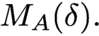 $M_A(\delta ).$
More generally, under a suitable condition on parameters
 $\delta $
, one can prove that any solution of
 $M_A(\delta )$
has an Euler integral representation (see [Reference Gel’fand, Kapranov and Zelevinsky10]).
Let
 $\pi :X=(\mathbb {G}_m)_x^n\times \mathbb {A}^N_z\setminus \bigcup _{l=1}^k\{ (x,z)\mid h_{l,z^{(l)}}(x)=0\}\rightarrow \mathbb {A}^N_z=Y$
be the projection, where subscripts stand for coordinates. We define an algebraic connection of the trivial bundle over X by
 $\nabla =\Phi ^{-1}\circ \nabla =\Phi ^{-1}\circ d_{(x,z)}\circ \Phi .$
We denote by
 $\mathbb {Z} A$
the sublattice of
 $\mathbb {Z}^{(n+k)\times 1}$
spanned by column vectors of A. If
 $\mathbb {Z} A=\mathbb {Z}^{(n+k)\times 1}$
,
 $\delta $
is nonresonant in the sense of [Reference Gel’fand, Kapranov and Zelevinsky10], and
 $\gamma _l\notin \mathbb {Z}$
for any
 $l=1,\dots ,k$
, we have the regularization isomorphism
 $\int _{\pi !}(\mathcal {O}_X,\nabla )\overset {\sim }{\rightarrow }\int _{\pi }(\mathcal {O}_X,\nabla )$
and a canonical isomorphism
 $M_A(\delta )\simeq \int _{\pi }(\mathcal {O}_X,\nabla )$
by [Reference Matsubara-Heo19, Theorem 2.12]. Note that the regularization condition is, in general, violated if any of
 $\gamma _l$
is an integer (see [Reference Matsubara-Heo19, Remark 2.14]). If we denote by U the Newton nondegenerate locus of
 $M_A(\delta )$
,
 $M_A(\delta )$
is a connection on U (see [Reference Adolphson1, Lemma 3.3]).
Now, let us fix a basis
 $\{\phi _i(z)\}_{i=1}^r\subset \int ^0_{\pi }(\mathcal {O}_X,\nabla )\restriction _{U}$
and a basis
 $\{\psi _i(z)\}_{i=1}^r\subset \int ^0_{\pi }(\mathcal {O}_X,\nabla ^{\vee })\restriction _{U}$
. By using the relative de Rham complex, we can explicitly compute the connection
 $\nabla ^{GM}$
of
 $\int ^0_{\pi }(\mathcal {O}_X,\nabla )\restriction _{U}$
via the formula
 $$ \begin{align} \nabla^{GM}\phi=d_z\phi-\displaystyle\sum_{j,l}\gamma_l\frac{x^{\textbf{ a}^{(l)}(j)}}{h_{l,z^{(l)}}(x)}dz_j^{(l)}\wedge\phi \end{align} $$
for any
 $\phi \in \operatorname {\mathrm {H}}^n\left ( (\mathbb {G}_m)^n_x\times U;\left (\Omega ^\bullet _{(\mathbb {G}_m)^n_x\times U/U}\left (*\cup _{l=1}^k\{ h_{l,z^{(l)}}(x)=0\}\right ),\nabla _x\right )\right )=\int ^0_{\pi }(\mathcal {O}_X,\nabla )\restriction _{U}$
. We have a similar formula for the connection
 $\nabla ^{\vee GM}$
of
 $\int ^0_{\pi }(\mathcal {O}_X,\nabla ^{\vee })\restriction _{U}$
. These bases as well as the connection matrices
 $\nabla ^{GM}=d_z+\Omega $
and
 $\nabla ^{\vee GM}=d_z+\Omega ^\vee $
can explicitly be constructed via Gröbner bases (see [Reference Hibi, Nishiyama and Takayama15, Theorem 2]). Note that there is an isomorphism induced by the correspondence
 $M_A(\delta )\ni [1]\mapsto [\frac {dx}{x}]\in \int _{\pi }^0(\mathcal {O}_X,\nabla )$
(see [Reference Matsubara-Heo19, Corollary 3.4]). When A is a matrix of the form (3.5), the associated GKZ system is regular holonomic (see [Reference Hotta16]). In [Reference Matsubara-Heo19], the intersection numbers for a basis of the twisted homology group for the GKZ system associated to a matrix A of the form (3.5) admitting a unimodular regular triangulation are determined when parameters are generic (see [Reference Matsubara-Heo19, Theorem 8.1]). The irreducibility of the GKZ system is proved under the nonresonance condition (see [Reference Beukers4], [Reference Gel’fand, Kapranov and Zelevinsky10], and [Reference Schulze and Walther27]). Note that irreducibility of a regular holonomic
 $\mathcal {D}$
-module is equivalent to that of the corresponding perverse sheaf by Riemann–Hilbert correspondence (see [Reference Hotta, Takeuchi and Tanisaki17, Theorem 7.2.5]). Algorithms for finding rational solutions have been studied by several approaches (see, e.g., [Reference Oaku, Takayama and Tsai24] and its references). These results together with our Theorem 2.1 yield the following theorem.
Theorem 3.2. Given a matrix
 $A=(a_{ij})$
as in (3.5) admitting a unimodular regular triangulation T. When parameters are nonresonant,
 $\gamma _l\notin \mathbb {Z}$
, and moreover the set of series solutions with respect to T is linearly independent, the intersection matrix of the twisted cohomology group of the GKZ system associated to the matrix A can be algorithmically determined.
We rename
 $(z_j^{(l)})_{j,l}$
as
 $(z_i)_i$
and denote
 $\frac {\partial }{\partial z_i}$
by
 $\partial _{i}$
. The action of a differential operator to a function is denoted by
 $\bullet $
. In other words,
 $\partial _{i}\bullet f$
means
 $\frac {\partial f}{\partial z_i}$
. Moreover, we denote by
 $\Omega _i$
the coefficient matrix of
 $\Omega $
with respect to the
 $1$
-form
 $dz_i$
. The algorithm we propose is summarized as follows.
-
1. Obtain a Pfaffian system
 $\partial _{i} + \Omega _i$
from the GKZ hypergeometric ideal defining
$M_A(\delta )$
generated by It is well known that this step can be performed by a Gröbner basis computation in the ring of differential operators with rational function coefficients. See, for example, [Reference Hibi14, 6.2, 7.4.2].
$$ \begin{align*} & \sum_j a_{ij} z_j \partial_{j} +\delta_i, \quad i=1, \ldots, n+k, \\ & \partial_{}^u - \partial_{}^v, \quad Au=Av, u,v \in \textbf{ N}_0^N. \end{align*} $$
-
2. Find a nonzero rational function solution I of the secondary equation,
To be more precise, see, for example, [Reference Oaku, Takayama and Tsai24] and its references.
$$ \begin{align*} \partial_{i}\bullet I - {}^t\Omega_i I - I \Omega_i^\vee =0, \quad i=1, \ldots, N. \end{align*} $$
-
3. Determine the constant multiple of I by the twisted period relation (2.6). To be more precise, we use [Reference Matsubara-Heo19, Theorem 8.1].


Let G be the Gröbner basis of the GKZ hypergeometric ideal obtained in step 1. The set of the standard monomials for G, which is the set of monomials in
 $\partial _{}$
that are not divisible by the initials of the elements of G, is of the form
 $\{ \partial _{}^s \,|\, s \in S \subset \textbf { N}_0^N\}$
(see, e.g., [Reference Hibi14, 6.1]). The basis of the twisted cohomology groups corresponding to G is obtained by applying these
 $\partial _{}^s$
’s to the kernel function of (3.1) and dividing it by (3.2).
Example 3.3. Let us determine algorithmically the intersection matrix of the twisted cohomology group for a matrix standing for the hypergeometric function
 ${}_2F_1$
, which was studied by [Reference Cho and Matsumoto6] and [Reference Matsumoto22] with geometric methods. We put
 $$ \begin{align*} A=\left( \begin{array}{cc|cc} 1 & 1 & 0 & 0 \\ \hline 0 & 0 & 1 & 1 \\ \hline 0 & 1 & 0 & 1 \end{array} \right) , \quad F=\left(\begin{array}{c} 1 \\ z_4 \partial_4 \end{array}\right). \end{align*} $$
Here,
 $\{1, \partial _{4}\}$
in the frame F is the set of the standard monomials of a Gröbner basis of the left ideal defining
 $M_A(\delta )$
. The bases of the twisted cohomology group corresponding to the frame F is
 $\left \{ \frac {dx}{x}, z_4 \frac {\partial \log {\Phi }}{\partial z_4} \frac {dx}{x}= \frac {-\gamma _2 z_4 dx}{(z_3+z_4 x)x} \right \}\subset \int ^0_{\pi }(\mathcal {O}_X,\nabla )\restriction _{U}$
and
 $\left \{ \frac {dx}{x}, z_4 \frac {\partial \log {\Phi }^{-1}}{\partial z_4} \frac {dx}{x}= \frac {\gamma _2 z_4 dx}{(z_3+z_4 x)x} \right \}\subset \int ^0_{\pi }(\mathcal {O}_X,\nabla ^{\vee })\restriction _{U}$
, where
 ${\Phi } = (z_1+z_2 x)^{-\gamma _1} (z_3 + z_4 x)^{-\gamma _2} x^c$
. The expression
 ${\nabla ^{GM}_{\partial _{z_4}}} \left [ \frac {dx}{x} \right ] = \frac {-\gamma _2 z_4 dx}{(z_3+z_4 x)x}$
is obtained by the exchange of
 $\partial _{z_4}$
and the integral sign as
 $$ \begin{align*} & \partial_{z_4} \bullet \int_\Gamma (z_1+x z_2)^{-\gamma_1} (z_3 + x z_4)^{-\gamma_2} x^c \cdot \frac{dx}{x} \\ &= \int_\Gamma (z_1+x z_2)^{-\gamma_1} (z_3 + x z_4)^{-\gamma_2} x^c \cdot \frac{-\gamma_2 z_4}{z_3+z_4 x} \frac{dx}{x} \end{align*} $$
and the perfectness of the twisted homology and cohomology groups. The other expressions can be obtained analogously. Generally speaking, through the connection
 $\nabla ^{GM}$
in (3.6), we can define an action of the Weyl algebra
 $D_N$
on
 $\int _\pi ^0 (\mathcal {O}_X,\nabla )$
; the action of
 $\partial _{z_i}$
is given by
 $\nabla ^{GM}_{\partial _{z_i}}$
. When
 ${\cal S}$
is the set of the standard monomials of a Gröbner basis of the left ideal defining
 $M_A(\delta )$
,
 $\left \{ s \bullet \left [ \left . \frac {dx}{x} \right ] \,\right |\, s \in {\cal S} \right \}$
is a free basis of
 ${\cal O}_{U'}$
-module
 $\int _\pi ^0 (\mathcal {O}_X,\nabla )|_{U'} \simeq M_A(\delta )|_{U'}$
, where
 $U'$
is the complement of the singular locus of
 $\Omega _i$
’s in Theorem 3.2 associated to the Gröbner basis.
Now, we set
 $z_1=z_2=z_3=1$
because of two reasons. The first reason is that the solutions of the GKZ system can be expressed as a composition of rational functions and transcendental functions of one variable by the homogeneity condition (first-order operators in
 $M_A(\delta )$
); see, e.g., [Reference Saito, Sturmfels and Takayama26, Proposition 1.3, 7]). The second reason is that if we do not set these
 $z_i$
’s to
 $1$
, the procedure to get a rational solution requires more computational resources, which are wasteful because of the homogeneity condition. For the frame F, we have the following connection and dual connection matrices:
 $$ \begin{align*} \Omega=\left( \begin{array}{cc} 0& \frac{ - c\gamma_2} { {z}_{4}- 1} \\ \frac{ 1} { {z}_{4}}& \frac{ -( c+ {\gamma}_{2}) {z}_{4}+c- {\gamma}_{1}} { {z}_{4} ( {z}_{4}- 1)} \\ \end{array} \right) dz_4, \end{align*} $$
 $$ \begin{align*} \Omega^\vee =\left( \begin{array}{cc} 0& \frac{ - c\gamma_2} { {z}_{4}- 1}\\ \frac{ 1} { {z}_{4}} & \frac{ ( c+ {\gamma}_{2}) {z}_{4}-c+ {\gamma}_{1}} { {z}_{4} ( {z}_{4}- 1)} \\ \end{array} \right) dz_4. \end{align*} $$
These can be obtained by a Gröbner basis of the hypergeometric ideal
 $M_A(\delta )$
(see, e.g., [Reference Hibi14, Chapter 6] and [Reference Saito, Sturmfels and Takayama26]). We find the following rational solution of the secondary equation
 $ d_{z_4} I - {}^t \Omega I - I \Omega ^\vee =0$
.
 $$ \begin{align*} I= \left( \begin{array}{cc} 1& \frac{ c\gamma_2} { \gamma_1+\gamma_2} \\ \frac{ -c\gamma_2} { \gamma_1+\gamma_2}& \frac{ c\gamma_2 ( {\gamma}_{1}- c)} {\gamma_1+\gamma_2 } \end{array} \right). \end{align*} $$
Let us utilize the quadratic relation of [Reference Matsubara-Heo19, Theorem 8.1] to determine the constant multiple of I. Let T be a unimodular triangulation
 $\{123,234\}$
. From the relation, we have
 $$ \begin{align*}\gamma_1 \gamma_2 \sum_{\sigma \in T} \frac{\pi^{3}}{\sin \pi A_\sigma^{-1} \delta} \varphi_{\sigma,0}(z; \delta) \varphi_{\sigma,0}(z; -\delta) = \frac{\langle \frac{dx}{x}, \frac{dx}{x} \rangle_{ch}}{ 2 \pi \sqrt{-1}}, \end{align*} $$
where
 $\varphi _{\sigma ,0}(z;\delta )$
is the series solution of the form
 $$ \begin{align*} \sum_{k \in \textbf{ N}_0} \frac{z^{kL+\rho}}{\prod_{i=1}^4 \Gamma(1+\rho_i+ k L_i)} , \quad L=(1,-1,-1,1), A \rho + \delta =0, \rho_i = 0 \ \text{when}\ i\not\in \sigma \end{align*} $$
and
 $A_\sigma $
is the submatrix of A constructed by taking the columns standing for
 $\sigma $
. For example, when
 $\sigma =234$
,
 $A_\sigma $
is the
 $3 \times 3$
matrix of which columns are the second, third, and fourth columns of A. The constant term of the left-hand side is
 $$ \begin{align} \frac{1}{\gamma_1-c} \left( \frac{\gamma_1}{c} + \frac{\gamma_2}{c-\gamma_1-\gamma_2} \right) = \frac{ - ( \gamma_{1}+ \gamma_{2})} { {c} ( {c}- \gamma_{1}- \gamma_{2})} \end{align} $$
by utilizing the rule
 $\Gamma (1+z)\Gamma (1-z)=z \frac {\pi }{\sin \pi z}$
. We multiply a constant to I, so that the
 $(1,1)$
element is equal to the constant (3.7)
 $\times 2 \pi \sqrt {-1}$
. Thus, we obtain the following intersection matrix of the twisted cohomology group:
 $$ \begin{align} 2 \pi \sqrt{-1} \left( \begin{array}{cc} \frac{ - ( {\gamma}_{1}+ {\gamma}_{2})} { {c} ( {c}- {\gamma}_{1}- {\gamma}_{2})}& \frac{ - {\gamma}_{2}} { {c}- {\gamma}_{1}- {\gamma}_{2}} \\ \frac{ {\gamma}_{2}} { {c}- {\gamma}_{1}- {\gamma}_{2}}& \frac{ {\gamma}_{2} ( {c}- {\gamma}_{1})} { {c}- {\gamma}_{1}- {\gamma}_{2}} \\ \end{array} \right). \end{align} $$
We conclude this section with simple observations on the cohomology intersection numbers associated to GKZ system. The first observation is on the dual fan of the Newton polytope of the LCM of the denominators (common denominator) of the entries of
 $I_{ch}$
. To begin with, we recall the basic notion of Newton polytope (see [Reference Gel’fand, Kapranov and Zelevinsky11, Chapter 6]). Let
 $f(z)=\sum _\alpha f_\alpha z^\alpha $
be a polynomial in
 $z=(z_1,\dots ,z_N)$
. The Newton polytope
 ${\textrm {New}}(f)$
is the convex hull of the index set
 $\{\alpha \mid f_\alpha \neq 0\}$
in
 $\mathbb {R}^{N\times 1}$
. For any convex polytope P in
 $\mathbb {R}^{N\times 1}$
and its face F, its normal cone
 $N_F(P)$
is defined to be the set of
 $\omega \in (\mathbb {R}^{N\times 1})^*=\mathbb {R}^{1\times N}$
such that the face determined by the vector
 $-\omega $
is F (
 $\langle -\omega, x\rangle $
takes the maximum on F while
 $x\in P$
). The dual fan of the Newton polytope
 ${\textrm {New}}(f)$
is denoted by
 ${\textrm {N}}(f)$
. Now, let us denote by
 $E_A(z)$
the product of principal
 $A_{\Gamma }$
-discriminants for any face
 $\Gamma $
of
 ${\textrm {New}}(A)$
(see [Reference Gel’fand, Kapranov and Zelevinsky11, Chapter 9 and Definition 1.2]). Here,
 ${\textrm {New}}(A)$
is the convex hull of column vectors of A. Since the secondary equation is a tensor product of
 $M_A(\delta )$
and
 $M_A(-\delta )$
, its singular locus is contained in the vanishing locus of
 $E_A(z)$
. If
 $g(z)$
denotes the common denominator of
 $I_{ch}$
, we have
 $\{ g(z)=0\}\subset \{ E_A(z)=0\}$
. By Hilbert’s nullstellensatz, there is a polynomial
 $h(z)$
and a positive integer l such that
 $E_A(z)^l=g(z)h(z)$
. Taking their Newton polytopes, we have
 ${\textrm {New}}(E_A^l)={\textrm {New}}(g)+{\textrm {New}}(h)$
. Here,
 $+$
is the Minkowski sum of convex polytopes. If we take their dual fans, we see that the left-hand side gives the secondary fan (see [Reference Gel’fand, Kapranov and Zelevinsky11, Chapters 7 and 10, Proposition 1.5, and Theorem 1.4]), whereas the right-hand side is a fan which is a refinement of
 ${\textrm {N}}(g)$
. Summing up all the arguments above, we obtain the following theorem.
Theorem 3.4. Suppose that the parameter
 $\delta $
is nonresonant and
 $\gamma _l\notin \mathbb {Z}$
for any
 $l=1,\dots ,k$
. Let g be the common denominator of
 $I_{ch}$
. Then, the secondary fan is a refinement of
 ${\textrm {N}}(g)$
.
Note that by [Reference Gel’fand, Kapranov and Zelevinsky11, Chapter 6 and Corollary 1.6], there is an injective correspondence from open cones of
 ${\textrm {N}}(g)$
to convergence domains of Laurent series expansions of
 $\frac {1}{g(z)}$
.
The second observation is on how the cohomology intersection number depends on the parameters
 $\delta $
. In Example 3.3, the basis F depends rationally on the parameters
 $\delta $
. In this case, the cohomology intersection numbers are rational functions in both the variables z and the parameters
 $\delta $
with coefficients in the field of rational numbers
 $\mathbb {Q}$
. Let us formulate the observation above. For any field extension
 $K\subset \mathbb {C}$
of
 $\mathbb {Q}$
, we set
 $(\mathbb {G}_m(K))^n_x={\textrm {Spec}}\left ( K[x_1^\pm ,\dots ,x_n^\pm ]\right )$
. Since the (reduced) defining equation
 $E_A(z)$
of the complement
 $Z=\mathbb {A}^N\setminus U$
is a rational polynomial, we can also consider a reduced scheme
 $U(K)$
defined over K whose base change to
 $\mathbb {C}$
is isomorphic to U. We denote by
 $D_{U(K)}$
the ring of differential operators on
 $U(K)$
. Any element P of
 $D_{U(K)}$
is a finite sum
 $P=\frac {1}{E_A(z)^l}\sum _\alpha a_\alpha (z)\partial ^\alpha $
, where
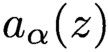 $a_\alpha (z)$
is a polynomial with coefficients in K and l is an integer.
Theorem 3.5. Suppose that
 $\delta $
is nonresonant,
 $\gamma _l\notin \mathbb {Z}$
, and A as in (3.5) admits a unimodular regular triangulation T. Then, for any
 $P_1,P_2\in D_{U(\mathbb {Q}(\delta ))}$
, the cohomology intersection number
 $\frac {\langle P_1\cdot \frac {dx}{x},P_2\cdot \frac {dx}{x}\rangle _{ch}}{(2\pi \sqrt{-1})^n}$
belongs to the field
 $\mathbb {Q}(\delta )(z)$
.
Proof. By the definition of the action of the ring
 $\mathbb {Q}(\delta )\langle z,\partial _z\rangle $
, it is enough to show that the function
 $I(z;\delta )= \frac {\langle x^{\textbf { a}}h^{\textbf { b}}\frac {dx}{x},x^{\textbf { a}^\prime }h^{\textbf { b}^\prime }\frac {dx}{x}\rangle _{ch}} {(2\pi \sqrt {-1})^n} $
belongs to the field
 $\mathbb {Q}(\delta )(z)$
. Here,
 $\textbf { a}=(a_1,\dots ,a_n),\textbf { a}^{\prime }\in \mathbb {Z}^n$
,
 $\textbf { b}=(b_1,\dots ,b_k),\textbf { b}^{\prime }\in \mathbb {Z}^k$
, and
 $x^{\textbf { a}}h^{\textbf { b}}=x_1^{a_1}\cdots x_n^{a_n}h_1^{b_1}\cdots h_k^{b_k}$
. Due to [Reference Ando, Esterov and Takeuchi2, Lemma 3.2], we may assume that the parameter
 $\delta $
is generic, so that the formula [Reference Matsubara-Heo19, Theorem 8.1] holds. Let B be an
 $N\times (N-n-k)$
integer matrix whose column vectors generate the kernel lattice
 $ \operatorname {\mathrm {Ker}}(A\times :\mathbb {Z}^{N}\rightarrow \mathbb {Z}^{n+k})$
and are compatible with the regular triangulation T in the sense of [Reference Gel’f, Kapranov and Zelevinsky9]. We take an
 $(N-n-k)\times N$
integer matrix C such that
 $CB$
is an identity matrix. We define a morphism
 $j_A:(\mathbb {C}^*)^{n+k}\rightarrow (\mathbb {C}^*)^N$
by
 $j_A(t)=t^A$
and a morphism
 $\pi _B:(\mathbb {C}^*)^N\rightarrow (\mathbb {C}^*)^{N-n-k}$
by
 $\pi _B(z)=z^B$
. Note that the morphism
 $j_A$
combined with the product structure of
 $(\mathbb {C}^*)^N$
induces an action of
 $(\mathbb {C}^*)^{n+k}$
on
 $(\mathbb {C}^*)^N$
. For any
 $t=(t_1,\dots ,t_{n+k})$
in
 $(\mathbb {C}^*)^{n+k}$
, we write
 $\tau _1=(t_1,\dots ,t_k)$
and
 $\tau _2=(t_{k+1},\dots ,t_{n+k})$
. By [Reference Matsubara-Heo19, Theorem 8.1], we have a formula
 $I(j_A(t)z;\delta )=\tau _1^{\boldsymbol {b+b}^{\prime }}\tau _2^{\boldsymbol {a-a}^{\prime }} I(z;\delta ).$
Taking into account this homogeneity property and the exact sequence
 $$ \begin{align} 1\rightarrow(\mathbb{C}^*)^{n+k}\overset{j_A}{\rightarrow}(\mathbb{C}^*)^{N}\overset{\pi_B}{\rightarrow}(\mathbb{C}^*)^{N-n-k}\rightarrow 1, \end{align} $$
we only have to show that
 $I_1(\zeta ;\delta )\overset {def}{=}I(\zeta ^C;\delta )\in \mathbb {Q}(\delta )(z)$
. Here,
 $\zeta $
is a coordinate of
 $({\mathbb {C}}^*)^{N-n-k}$
. Note that the Laurent series expansion formula [Reference Matsubara-Heo19, Theorem 8.1] is valid when the absolute values of entries of
 $\zeta $
are all small. Since
 $I(z;\delta )$
is a solution of the secondary equation (2.9) and (2.9) is isomorphic to
 $M_A(\delta )\otimes M_A(-\delta )$
, for an appropriate nonnegative integer l and a polynomial
 $f(\zeta ;\delta )$
in
 $\zeta $
and a vector
 $\alpha _0\in {\textbf { N}_0}^{N-n-k}$
, we have
 $I_1(\zeta ;\delta )=\frac {f(\zeta ;\delta )}{\zeta ^{\alpha _0} E_A(\zeta ^C)^l}$
. Note that
 $E_A(z)\in \mathbb {Q}[z]$
. We write
 $f(\zeta ;\delta )=\sum _{i=1}^df_i(\delta )\zeta ^{\alpha _i}$
, where
 $\alpha _i$
are elements of
 ${\textbf { N}_0}^{N-n-k}$
. By choosing a suitable vector
 $\phi =(\phi _1,\dots ,\phi _{N-n-k})\in {\textbf { N}_0}^{N-n-k}$
and by rearranging
 $\alpha _i$
if necessary, we may assume
 $0\leq \langle \phi ,\alpha _1\rangle <\cdots <\langle \phi ,\alpha _d\rangle $
. Here,
 $\langle \bullet ,\bullet \rangle $
is the dot product of vectors. We set
 $g(\zeta )=E_A(\zeta ^C)^l$
. For a complex variable
 $\xi $
, we write
 $\xi ^\phi =(\xi ^{\phi _1},\dots ,\xi ^{\phi _{N-n-k}}).$
We put
 $F(\xi )\overset {def}{=}f(\xi ^\phi ;\delta )=\xi ^{\langle \phi ,\alpha _0\rangle }g(\xi ^{\phi })I_1(\xi ^\phi ;\delta ).$
By [Reference Matsubara-Heo19, Theorem 8.1] and the fact that B is compatible with T, we see that
 $I_1(\xi ^\phi ;\delta )$
is a Laurent series in
 $\xi $
with coefficients in
 $\mathbb {Q}(\delta )$
. Since
 $F(\xi )=\sum _{i=1}^df_i(\delta )\xi ^{\langle \phi ,\alpha _i\rangle }$
, we obtain
 $f_i(\delta )\in \mathbb {Q}(\delta )$
. Thus, we have
 $f(\zeta ;\delta )\in \mathbb {Q}(\delta )[\zeta ]$
, hence we obtain
 $I_1(\zeta ;\delta )\in \mathbb {Q}(\delta )(z)$
.
For any field extension
 $K\subset \mathbb {C}$
of
 $\mathbb {Q}(\delta )$
, we define the symbol
 $\int ^0_{\pi }(\mathcal {O}_{X(K)},\nabla )\restriction _{U(K)}$
by
 $$ \begin{align} \mathbb{H}^n\left( (\mathbb{G}_m(K))^n_x\times U(K);\left(\Omega^{\bullet}_{(\mathbb{G}_m(K))^n_x\times U(K)/U(K)}\left(*\bigcup_{l=1}^k\{ h_{l,z^{(l)}}(x)=0\}\right),\nabla_x\right)\right), \end{align} $$
where
 $\mathbb {H}^n$
stands for the n-th hypercohomology group. By the formula (3.6),
 $\int ^0_{\pi }(\mathcal {O}_{X(K)},\nabla ) \restriction _{U(K)}$
naturally has a structure of
 $D_{U(K)}$
-module. When
 $\delta $
is nonresonant,
 $\gamma _l\notin \mathbb {Z}$
, and
 $K=\mathbb {Q}(\delta )$
, any element
 $[\phi ]\in \int _{\pi }^0(\mathcal {O}_{X(K)},\nabla )\restriction _{U(K)}$
can be written as
 $[\phi ]=P\cdot [\frac {dx}{x}]$
for some
 $P\in D_{K}$
. Therefore, we obtain the following theorem.
Theorem 3.6. Under the assumption of Theorem 3.5, the normalized cohomology intersection pairing
 $B=\frac {\langle \bullet ,\bullet \rangle _{ch}}{(2\pi \sqrt {-1})^n}$
defines a perfect bilinear pairing
 $$ \begin{align} \int^0_{\pi}(\mathcal{O}_{X(\mathbb{Q}(\delta))},\nabla)\restriction_{U(\mathbb{Q}(\delta))}\times\int^0_{\pi}(\mathcal{O}_{X(\mathbb{Q}(\delta))},\nabla^\vee)\restriction_{U(\mathbb{Q}(\delta))}\rightarrow\mathcal{O}_{U(\mathbb{Q}(\delta))} \end{align} $$
such that the formula (2.10) holds.
Therefore, when the parameter
 $\delta $
is generic, we can treat it as a formal symbol and we do not need to consider any algebraic extension of
 $\mathbb {Q}$
in our algorithm.
4 A period integral associated to a family of K3 surfaces [Reference Narumiya and Shiga23]
This section is a demonstration of our algorithmic method to obtain the intersection matrix of twisted cohomology groups and functional identities derived by the twisted period relation. The intersection matrix and some functional identities presented in this section have not been obtained by other methods. We also note that once we obtain the intersection matrix, the correctness modulo a constant multiple can be checked if it satisfies the secondary equation (2.9). Since the entries of the matrix are rational functions, it can be checked by computer algebra systems.
We consider an Euler integral
 $$ \begin{align} f(z)=\int_\Gamma u\frac{dx\wedge dy}{xy},\ u=(z_1x^3+z_2x^2y+z_3x^2y^{-1}+z_4x^2+z_5x)^{-c_1}x^{c_2}y^{c_3} \end{align} $$
under the nonresonance condition on c. This function is a solution of the GKZ system associated to the matrix
 $$ \begin{align*} \left(\!\!\begin{array}{c}1\\\textbf{ a}^{(1)}(j)\end{array}\!\right) = \left(\!\begin{array}{ccccc} 1 & 1 & 1 & 1 & 1 \\ 3 & 2 & 2 & 2 & 1 \\ 0 & 1 & -1 & 0 & 0 \\ \end{array}\!\right). \end{align*} $$
We can see that the sets of rational differential forms
 $$ \begin{align} \omega=\frac{dx \wedge dy}{xy}, \frac{\partial \log u}{\partial z_5} \omega, \frac{\partial \log u}{\partial z_4} \omega, \frac{\partial^2 u}{\partial z_5^2} \frac{1}{u} \omega \end{align} $$
and
 $$ \begin{align} \omega=\frac{dx \wedge dy}{xy}, \frac{\partial \log u^{-1}}{\partial z_5} \omega, \frac{\partial \log u^{-1}}{\partial z_4} \omega, \frac{\partial^2 (u^{-1})}{\partial z_5^2} u \omega \end{align} $$
are bases of the twisted cohomology groups and construct the connection matrices
 $d_z+\Omega $
and
 $d_z+\Omega ^\vee $
with these bases by Gröbner basis computation (see, e.g., [Reference Hibi14, Chapter 6]). When
 $c = \left (\begin {array}{c}1/2\\ 1+\varepsilon \\ \varepsilon \end {array}\right ) $
and
 $z_1=z_2=z_3=1$
(we make this specialization with the same reason mentioned in Example 3.3), we find by solving the secondary equation that the intersection matrix of the cohomology group is a scalar multiple of the matrix
 $$ \begin{align} I= \begin{pmatrix} 1& \frac{ - 4{\varepsilon}+ 1}{ 8{z}_{5}}& 0& \frac{ 4 \varepsilon^{ 2} + 3 \varepsilon- 1}{ 8{z}_{5}^{ 2} } \\ \frac{ 4 \varepsilon- 1}{ 8{z}_{5}}& \frac{ - 4 \varepsilon^{ 2} + \varepsilon}{ 8{z}_{5}^{ 2} }& 0& r_{24}\\ 0& 0& 0& r_{34}\\ \frac{ 4 \varepsilon^{ 2} - 5 \varepsilon+ 1}{ 8 {z}_{5}^{ 2} }&r_{42}&r_{43}&r_{44} \end{pmatrix}, \end{align} $$
where
 $r_{ij}$
are rational functions in the
 $z_4$
,
 $z_5$
, and
 $\varepsilon $
. Note that this I gives an example that
 $I_{ch}$
is not necessarily a constant matrix with respect to z. By [Reference Matsubara-Heo19, Theorem 8.1], we can see that the self-intersection number of the first form is
 $$ \begin{align} \left\langle \frac{dx \wedge dy}{xy}, \frac{dx \wedge dy}{xy} \right\rangle \ |_{z_1=z_2=z_3=1} = \frac{32}{1-16\varepsilon^2} (2 \pi \sqrt{-1})^2. \end{align} $$
Thus, the intersection matrix is equal to
 $ (2 \pi \sqrt {-1})^2 \frac {32}{1-16\varepsilon ^2} I$
, which gives quadratic relations of GKZ hypergeometric series. The whole intersection matrix of the twisted cohomology group is posted at our web page.Footnote
1
Let us show a quadratic relation by taking a restriction to
 $\{ z_1=z_2=z_3=z_5=1\}$
(see [Reference Narumiya and Shiga23]). In this case, we have three independent series
 $$ \begin{align} \varphi_{345}(1,1,1,z_4,1;c(\varepsilon))=z_4^{-\frac{1}{2}-2\varepsilon}\sum_{m,n\geq 0}\frac{(z_4^{-2})^{m+n}}{\Gamma(1+\varepsilon+n)\Gamma(\frac{1}{2}-2\varepsilon-2m-2n)\Gamma(1+\varepsilon+m)m!n!}, \nonumber\\\end{align} $$
 $$ \begin{align} &\varphi_{245}(1,1,1,z_4,1;c(\varepsilon))=\varphi_{134}(1,1,1,z_4,1;c(\varepsilon))\nonumber\\ =&z_4^{-\frac{1}{2}}\sum_{m,n\geq 0}\frac{(z_4^{-2})^{m+n}}{\Gamma(1-\varepsilon+n)\Gamma(\frac{1}{2}-2m-2n)\Gamma(1+\varepsilon+m)m!n!}, \end{align} $$
 $$ \begin{align} \varphi_{124}(1,1,1,z_4,1;c(\varepsilon))=z_4^{-\frac{1}{2}+2\varepsilon}\sum_{m,n\geq 0}\frac{(z_4^{-2})^{m+n}}{\Gamma(1-\varepsilon+n)\Gamma(\frac{1}{2}+2\varepsilon-2m-2n)\Gamma(1-\varepsilon+m)m!n!}.\nonumber\\ \end{align} $$
From our intersection matrix of the twisted cohomology group, we obtain the following quadratic relation (see [Reference Matsubara-Heo19, Theorem 8.1]):
 $$ \begin{align} &\frac{1}{2}\left\{ \frac{\pi^3}{\sin^2\pi\varepsilon\cos\pi(2\varepsilon)}\varphi_{345}(1,1,1,z_4,1;c(\varepsilon))\varphi_{345}(1,1,1,z_4,1;-c(\varepsilon))\right.\nonumber\\ &-\frac{2\pi^3}{\sin^2\pi\varepsilon}\varphi_{245}(1,1,1,z_4,1;c(\varepsilon))\varphi_{245}(1,1,1,z_4,1;-c(\varepsilon))\nonumber\\ &\left. +\frac{\pi^3}{\sin^2\pi\varepsilon\cos\pi(2\varepsilon)}\varphi_{124}(1,1,1,z_4,1;c(\varepsilon))\varphi_{124}(1,1,1,z_4,1;-c(\varepsilon))\right\}\nonumber\\ =&\frac{32}{(1-16\varepsilon^2)}. \end{align} $$
When
 $\varepsilon =0$
, the integral
 $f(z)$
reduces to the integral discussed in the context of mirror symmetry (see [Reference Narumiya and Shiga23]). It satisfies a rank
 $3$
system. We are interested in this case. Once we obtain the quadratic relation, we can take a limit
 $\varepsilon \rightarrow 0$
and get a quadratic relation for the case of the resonant parameter value. However, the set of the naive limits of
 $\varphi _{ijk}$
’s does not give a basis of the solution space of the rank
 $3$
system. We put
 $\alpha =\frac {\pi ^3}{\sin ^2\pi \varepsilon \cos \pi (2\varepsilon )}$
,
 $\beta =-\frac {\pi ^3}{\sin ^2\pi \varepsilon }$
,
 $$ \begin{align} \Phi_\varepsilon&=\Bigg(\varphi_{345}(1,1,1,z_4,1;c(\varepsilon)),\varphi_{245}(1,1,1,z_4,1;c(\varepsilon)),\nonumber\\ &\quad \varphi_{134}(1,1,1,z_4,1;c(\varepsilon)),\varphi_{124}(1,1,1,z_4,1;c(\varepsilon))\Bigg), \end{align} $$
and
 $$ \begin{align} \Phi^\vee_\varepsilon&=\Bigg(\varphi_{345}(1,1,1,z_4,1;-c(\varepsilon)),\varphi_{245}(1,1,1,z_4,1;-c(\varepsilon)),\nonumber\\ &\quad\varphi_{134}(1,1,1,z_4,1;-c(\varepsilon)), \varphi_{124}(1,1,1,z_4,1;-c(\varepsilon))\Bigg). \end{align} $$
Let us construct a set of linearly independent solutions by the Frobenius method from
 $\Phi _\varepsilon $
and
 $\Phi ^\vee _\varepsilon $
. When
 $\varepsilon \not = 0$
, the twisted period relation (4.9) can be written in the following form:
 $$ \begin{align} \Phi_\varepsilon \begin{pmatrix} \alpha&0&0&0\\ 0&\beta&0&0\\ 0&0&\beta&0\\ 0&0&0&\alpha \end{pmatrix} {}^t\Phi^\vee_\varepsilon =\frac{64}{(1-16\varepsilon^2)}. \end{align} $$
In order to obtain linearly independent solutions, we introduce a
 $4\times 4$
matrix Q defined by
 $$ \begin{align} Q= \begin{pmatrix} 1&-\varepsilon^{-1}&-\varepsilon^{-1}&\varepsilon^{-2}\\ 0&\varepsilon^{-1}&0&-\varepsilon^{-2}\\ 0&0&\varepsilon^{-1}&-\varepsilon^{-2}\\ 0&0&0&\varepsilon^{-2} \end{pmatrix}. \end{align} $$
This matrix Q is chosen, so that the set
 $$ \begin{align*} \lim_{\varepsilon \rightarrow 0} \varphi_{345},\ \lim_{\varepsilon \rightarrow 0} (\varphi_{245}-\varphi_{345})/\varepsilon= \lim_{\varepsilon \rightarrow 0} (\varphi_{134}-\varphi_{345})/\varepsilon,\ \lim_{\varepsilon \rightarrow 0} (\varphi_{345}-\varphi_{245}-\varphi_{134}+\varphi_{124})/\varepsilon^2 \end{align*} $$
is a basis of the solutions when
 $\varepsilon =0$
. This method is called the Frobenius method (see, e.g., [Reference Saito, Sturmfels and Takayama26, pp.22, 145]). We put
 $\tilde {\Phi }_\varepsilon =\Phi _\varepsilon Q$
and
 $\tilde {\Phi }^\vee _\varepsilon =\Phi ^\vee _\varepsilon Q$
. A simple computation shows that
 $\tilde {\Phi }=\tilde {\Phi }_\varepsilon \restriction _{\varepsilon \rightarrow 0}$
and
 $\tilde {\Phi }^\vee =\tilde {\Phi }^\vee _\varepsilon \restriction _{\varepsilon \rightarrow 0}$
are convergent and we have a limit formula:
 $$ \begin{align} \tilde{\Phi} \begin{pmatrix} 4\pi^3&0&0&\pi\\ 0&0&\pi&0\\ 0&\pi&0&0\\ \pi&0&0&0 \end{pmatrix} {}^t\tilde{\Phi}^\vee =64. \end{align} $$
The components of the vector
 ${\tilde \Phi }$
are as follows:
 $$ \begin{align} {\tilde \Phi}_1= \frac{1}{\sqrt{\pi } \sqrt{z_4}} \left(1+\frac{3}{2 z_4^2}+O\left(\left(\frac{1}{z_4}\right)^4\right) \right), \end{align} $$
 $$ \begin{align} {\tilde \Phi}_2 &= {\tilde \Phi}_3 = \frac{1}{\sqrt{\pi } \sqrt{z_4}} (\phi^{\prime}_{20} + (\log z_4) \phi^{\prime}_{21}), \end{align} $$
 $$ \begin{align} {\tilde \Phi}_4 &= \frac{1}{\sqrt{\pi } \sqrt{z_4}}(\phi^{\prime}_{40}+(\log z_4) \phi^{\prime}_{41} +(\log z_4)^2 \phi^{\prime}_{42}).\end{align} $$
The components of the vector
 ${\tilde \Phi }^\vee $
are as follows:
 $$ \begin{align} {\tilde \Phi}_1^\vee=\frac{2 \sqrt{z_4}}{\sqrt{\pi }}\left(1-\frac{1}{2 z_4^2}+O\left(\left(\frac{1}{z_4}\right)^4\right)\right), \end{align} $$
 $$ \begin{align} {\tilde \Phi}_2^\vee&={\tilde \Phi}_3^\vee=\frac{2 \sqrt{z_4}}{\sqrt{\pi }}(\phi_{20} + (\log z_4)\phi_{21}), \end{align} $$
 $$ \begin{align} {\tilde \Phi}_4^\vee&=\frac{2 \sqrt{z_4}}{\sqrt{\pi }}(\phi_{40} + (\log z_4)\phi_{41}+(\log z_4)^2 \phi_{42}). \end{align} $$
Here,
 $\phi _{ij}$
and
 $\phi ^{\prime }_{ij}$
are power series in
 $z_4^{-2}$
. We would like to note that coefficients of these power series are very complicated, but these satisfy a simple functional identity (4.14). Interested readers may refer to our Mathematica programs tperiod.m and fancy.m
Footnote
2
to obtain explicit expressions of coefficients of these series.
As for
 $\tilde {\Phi }_1$
, it can be related to Thomae’s and Gauß’s hypergeometric series by a simple transformation
 $$ \begin{align} \pi^{1/2} z_4^{1/2} {\tilde \Phi}_1(z_4)= {}_3 F_2\left(\substack{1/4,2/4,3/4 \\1,1}; 16/z_4^2\right) = \left({}_2F_1\left(\substack{1/8,3/8\\ 1};16/z_4^2\right)\right)^2 \end{align} $$
as was remarked in [Reference Narumiya and Shiga23]. Here, the second equality is the result of Clausen’s identity.
Appendix: A lemma on a stalk of a direct image
In this appendix, we prove the following lemma.
Lemma 4.1. Let
 $X,F$
be real manifolds, let
 $p:X\times F\rightarrow X$
, let
 $q:X\times F\rightarrow F$
be the canonical projections, and let
 $\mathcal {L}$
be a
 $\mathbb {Q}$
-local system on F. Then, for any
 $x\in X$
and any integer k, there is a canonical isomorphism
 $$ \begin{align} \left(R^kp_*({q^{-1}}\mathcal{L})\right)_x\simeq H^k\left( F, \mathcal{L}\right) \end{align} $$
under the natural identification
 $F\simeq \{ x\}\times F$
.
Proof . Since
 $R^kp_*({q^{-1}}\mathcal {L})$
is the sheaf associated to the presheaf
 $U\mapsto \operatorname {\mathrm {H}}^k\left ( p^{-1}(U),{q^{-1}}\mathcal {L}\right )$
, we see that the left-hand side of (4.22) is equal to
 $\underset {x\in U}{\varinjlim } \operatorname {\mathrm {H}}^k\left ( p^{-1}(U),{q^{-1}}\mathcal {L}\right )$
. Since X is a real manifold, we can find a fundamental system of neighborhoods of x consisting of balls in an Euclidian space. When U is a ball, by Künneth formula, we have a sequence of isomorphisms
 $ \operatorname {\mathrm {H}}^k\left ( p^{-1}(U),{q^{-1}}\mathcal {L}\right )\simeq \operatorname {\mathrm {H}}^0\left ( U,{\mathbb {Q}}\right )\otimes _{\mathbb {Q}} \operatorname {\mathrm {H}}^k\left ( F,\mathcal {L}\right )\simeq \operatorname {\mathrm {H}}^k\left ( F,\mathcal {L}\right ).$
Acknowledgments
Saiei-Jaeyeong Matsubara-Heo is supported by the Japan Society for the Promotion of Science’s (JSPS) Grants-in-Aid for Scientific Research (KAKENHI) Grant Number 19K14554, and Nobuki Takayama is supported by JSPS KAKENHI Grant Number 17K05279. Both of the authors are supported by the Japan Science and Technology Agency’s Core Research for Evolutional Science and Technology Grant Number JP19209317. Saiei-Jaeyeong Matsubara-Heo would like to thank Masatoshi Noumi for valuable comments. Corollary 2.2 is an outcome of the comments. He would also like to thank Frits Beukers for letting him know the paper [Reference Beukers and Jouhet5], where the authors discuss duality relations of univariate hypergeoemtric systems from a similar point of view. We deeply appreciate several comments of the reviewer for improving some explanations and for clarifying main points of our paper.



