


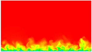





1. Introduction
The simulation of turbulent boundary layer (TBL) flows have a rich history spanning several decades with one of the pioneering direct numerical simulations (DNS) conducted by Spalart (Reference Spalart1988) for momentum thickness-based Reynolds numbers  $Re_\theta =300, 670$ and
 $1410$. As more computational resources have become available, several DNS have been published for zero pressure gradient (ZPG) TBL flows at significantly higher Reynolds numbers. For example, Schlatter et al. (Reference Schlatter, Örlü, Li, Brethouwer, Fransson, Johansson, Alfredsson and Henningson2009) performed the DNS of ZPG TBL up to
 ${Re}_\theta =2500$. Later Sillero, Jiménez & Moser (Reference Sillero, Jiménez and Moser2013) extended the available DNS simulation up to
 $Re_\theta =6680$. In addition to DNS, large eddy simulation (LES) have played a vital role in studying high Reynolds numbers TBL flows. Well-resolved LES up to
 ${Re}_\theta =4300$ were performed by Schlatter et al. (Reference Schlatter, Li, Brethouwer, Johansson and Henningson2010). Later, Eitel-Amor, Örlü & Schlatter (Reference Eitel-Amor, Örlü and Schlatter2014) extended the LES of spatially evolving ZPG TBL flows to
 ${Re}_\theta =8300$. Other works include the ones by Wu & Moin (Reference Wu and Moin2009) who simulated a ZPG boundary layer up to
 $Re_\theta =940$, which was later extended up to
 $Re_{\theta }=1950$ (Wu & Moin Reference Wu and Moin2010) and the work by Ferrante & Elghobashi (Reference Ferrante and Elghobashi2005) who reached up to
 $Re_\theta =2900$.
One of the straightforward approaches to simulate a TBL is to obtain conditions closely resembling a wind tunnel experiment which involves initiating a laminar boundary layer and subsequently introducing disturbances downstream. These disturbances can be simulated, for instance, through the use of forcing terms in the Navier–Stokes equations that are activated at the wall at an upstream location, which try to mimic the presence of sandpaper roughness at the wall, as one would do in a wind tunnel set-up (see, for example, Reshotko (Reference Reshotko2001), Marusic et al. (Reference Marusic, Chauhan, Kulandaivelu and Hutchins2015) and Tabatabaei et al. (Reference Tabatabaei, Vinuesa, Örlü and Schlatter2021)). However, such a simulation would take a significant distance downstream to develop to the real turbulence at the required Reynolds number with correct statistics (Tabor & Baba-Ahmadi Reference Tabor and Baba-Ahmadi2010; Dhamankar, Blaisdell & Lyrintzis Reference Dhamankar, Blaisdell and Lyrintzis2018). As Dhamankar et al. (Reference Dhamankar, Blaisdell and Lyrintzis2018) mentions in their review article, ‘this distance is variably referred to as the redevelopment region, adjustment length, recovery distance, adaptation distance’ or development length in the literature. In this work, we refer to it as the development length.
One of the main challenges in simulating spatially evolving TBLs, even on flat plates, is the construction of an inflow condition that quickly adapts to the desired turbulence status, in other words, one that requires shorter development lengths. Constructing a turbulent inflow that enables such a rapid transition to the expected turbulence behaviour is demanding in wall-bounded turbulence simulations, as it would avoid extra costs associated with simulating highly resolved regions upstream of the region of interest devoted just for developing the flow to the expected turbulent state. Several methods exist in the literature (a great overview of which can be found in the work by Wu (Reference Wu2017)), with varying degrees of computational cost. One approach is to conduct precursor auxiliary simulations and map time-dependent, statistically stationary fields onto the inflow of the turbulence simulation (Malm et al. Reference Malm, Schlatter, Henningson, Schrader and Mavriplis2012; Vinuesa et al. Reference Vinuesa, Schlatter, Malm, Mavriplis and Henningson2015; Munters, Meneveau & Meyers Reference Munters, Meneveau and Meyers2016; Mukha & Liefvendahl Reference Mukha and Liefvendahl2017), as we discuss further below, we employ this method in part of this current work. The rescaling–recycling method by Lund, Wu & Squires (Reference Lund, Wu and Squires1998), and advanced versions like the one by Ferrante & Elghobashi (Reference Ferrante and Elghobashi2004), is used in the precursor simulation where one extracts a cross-stream two-dimensional (2-D) slice of velocity field downstream of the inlet, rescales it and reintroduces it into the inlet. A more common approach is to have rescaling–recycling in the main simulation (Araya et al. Reference Araya, Castillo, Meneveau and Jansen2011). Another way is the synthetic turbulent inflow generation method, where random fluctuations are added into the inflow based on the turbulence statistics at the required Reynolds number. Several methods aligned with this approach have been proposed, such as the synthetic random Fourier method by Le, Moin & Kim (Reference Le, Moin and Kim1997), the synthetic coherent eddy method by Jarrin et al. (Reference Jarrin, Benhamadouche, Laurence and Prosser2006), the synthetic volume-force method by Spille & Kaltenbach (Reference Spille and Kaltenbach2001) and Schlatter & Örlü (Reference Schlatter and Örlü2012) and the divergence-free generalized synthetic eddy method (gSyEM) (Poletto et al. Reference Poletto, Revell, Craft and Jarrin2011). Selent et al. (Reference Selent, Wenzel, Rist and Schmidt2020) proposed a turbulence inflow method based on synthetic volume forcing where the spatial and temporal properties of the eddies were obtained from resolvent mode analysis of turbulent mean flow data. In recent years, due to the rapid development of the use of machine learning in turbulence simulations, inflow generators based on machine learning models have been explored. Fukami et al. (Reference Fukami, Nabae, Kawai and Fukagata2019) showed the feasibility of using convolutional neural networks to generate inflow conditions. Recently, Yousif, Yu & Lim (Reference Yousif, Yu and Lim2022) utilized a combination of a multiscale convolutional autoencoder with a subpixel convolution layer having a physical constraints-based loss function and a long short-term memory model to generate turbulent inflow conditions from turbulent channel flow data. Yousif et al. (Reference Yousif, Zhang, Yu, Vinuesa and Lim2023) used a combination of a transformer and a multiscale-enhanced super-resolution generative adversarial network to predict velocity fields normal to the streamwise direction of a spatially developing TBL in the range of  $Re_{\theta }=661\unicode{x2013}1502$. Some interesting works have been done by using experimental data as inflow condition to simulations in the framework of the so-called data assimilation methods. For instance, Ezhilsabareesh, Callum & Soria (Reference Ezhilsabareesh, Callum and Soria2024) and Appelbaum et al. (Reference Appelbaum, Ohno, Rist and Wenzel2021) used particle image velocimetry and particle tracking velocimetry, respectively, to study their potential effectiveness as inflow conditions in simulations.
There is a general consensus (Tabor & Baba-Ahmadi Reference Tabor and Baba-Ahmadi2010) within the computational fluid dynamics (CFD) community about inflow simulations based on mapping time-dependant velocity fields from precursor auxiliary simulations being better, in terms of reducing the development length, compared with the other methods mentioned above. However, this method is computationally intensive, as either the precursor simulation has to be run simultaneously along with the main simulation, or the precursor simulation has to be previously run for a significantly long time duration and its required velocity slices have been saved onto the disk. This results in large storage requirements as well as input/output bottlenecks when reading the data from the disk during the main simulation. A potential way to reduce these costs associated with the precursor method, while still retaining its advantages of providing a realistic inflow condition, would be to create a reduced-order model (ROM). Such a ROM should be designed to represent the behaviour of the time-dependent inflow velocity fields (i.e. the spatiotemporal evolution of coherent structures at a given location) so that this model can then be incorporated within the main simulation code. This would help to avoid reading velocity fields from disk. Previously, Gloerfelt & Garrec (Reference Gloerfelt and Garrec2008) used a proper orthogonal decomposition (POD)-Galerkin method to create a ROM-based inflow that is suitable for aeroacoustic studies. Perret et al. (Reference Perret, Delville, Manceau and Bonnet2008) used a POD combined with experimental data from particle image velocimetry measurements to provide an inflow condition. The objective of this work is to propose and evaluate a ROM-based inflow method for TBLs, with a specific focus on the time coefficients.
In this work, we discuss the possibility of using vector autoregressive (VAR) models as a means of efficiently and accurately generating turbulent inflow fields for spatially developing TBLs. VAR is a method that has received limited attention in the context of fluid dynamics and turbulent flows (Hæpffner, Naka & Fukagata Reference Hæpffner, Naka and Fukagata2011). However, it is a well-established technique for the analysis and forecasting of multivariate time series data in fields such as economics, (see, for example, Hatemi-J (Reference Hatemi-J2004), Lütkepohl (Reference Lütkepohl2005) and Hacker & Hatemi-J (Reference Hacker and Hatemi-J2008)), and natural sciences (Keng et al. Reference Keng, Shan, Shimizu, Imoto, Lateh and Peng2017). A rare application of VAR for the generation of synthetic turbulent wind fields was performed by Elagamy et al. (Reference Elagamy, Gallego-Castillo, Cuerva-Tejero, Lopez-Garcia and Avila-Sanchez2023), who employed VAR in the eigenanalysis of the companion matrix of a first-order vector autoregressive model.
Since VAR is a linear technique, its application to the modelling of nonlinear phenomena such as three-dimensional turbulence can be quite involved. In order to simplify this, while ensuring that the important temporal cross-correlations are not lost, a VAR model is constructed using the time coefficients from the POD of velocity fields. For the spatially evolving ZPG TBL flow, a 2-D cross-section at a certain  ${Re}_{\theta }$ is selected. This cross-section represents the desired spatial location for initializing the turbulent inflow plane in the main simulation. A POD of the velocity field at this designated cross-section is performed using snapshots of the 2-D field collected over a statistically significant time interval. Since the flow is homogeneous in the spanwise direction, a Fourier transform is first performed in the spanwise direction and then POD is performed for every spanwise wavenumber. The time coefficients of the POD modes are then used as inputs to the VAR model. Our study shows that in cases where the time series exhibits a high correlation, a VAR model could be fit easily, and the time series could be extrapolated to any desired lengths while retaining the statistical properties of the original turbulent flow used as input. The VAR-generated time coefficients coupled with the original POD modes can then be used to reconstruct turbulent velocity fields at the chosen streamwise location, for indefinite time.
In order to assess the effectiveness of the proposed method to provide inflow conditions for ZPG TBLs, we conduct a TBL simulation using the inflow velocity fields reconstructed from VAR-generated time coefficients with POD modes. We then compare it with a series of main simulations derived from complete velocity fields (i.e. where no reduced-order modelling is performed) as well as those reconstructed using the time coefficients from certain subsets of the POD modes. The results detailed in the present study emphasize the potential of VAR as a tool for generating synthetic turbulence with a number of applications including efficient and accurate inflow generation in scale-resolving turbulence simulations.
The remainder of this article is organized as follows. The methodologies and workflow are explained in § 2. Then the details of the POD and VAR applied to the velocity fields of a ZPG TBL flow at  $Re_\theta =790$ are described in § 3. This is followed by results and discussion in § 4, where first the VAR is validated in § 4.1 and then results from the main simulations are shown in § 4.2. This is followed by the results of applying VAR to the time coefficients of a higher Reynolds number (i.e.
 $Re_\theta =2240$) data set in § 4.3 and the application of VAR to smoothen spectra in § 4.4. Finally, concluding remarks and future works are provided in § 5.
2. Workflow and simulation set-up
2.1. Workflow
As shown in the schematic in figure 1, two CFD solvers are involved in this workflow: SIMSON (Chevalier et al. Reference Chevalier, Schlatter, Lundbladh and Henningson2007) and Nek5000 (Fischer, Lottes & Kerkemeier Reference Fischer, Lottes and Kerkemeier2008). More details regarding each of them are described in §§ 2.2 and 2.3, respectively. The former is used for the precursor simulation, and the latter is used for the main simulation where the inflow Dirichlet condition is applied. The inflow condition can be applied either directly, as described in § 2.4.1, or after creating a reduced-order representation as described in § 2.4.2. Then the main simulation is used to study the corresponding development lengths in a flat plate simulation.
An overview of the workflow adopted showing different procedures chosen for the different main simulations starting from the same precursor simulation. Here ‘baseline’ refers to the main simulation where the time dependant 2-D velocity slices from the precursor simulation are used as inflow conditions without creating any low-order representation, and hence establishing a baseline to compare with the other main simulations. On the other hand, ‘ $5$’ and ‘
 $30$’ refer to the number of POD modes per wavenumber (m.p.w.) used. Among the main simulations, the ones named as ‘POD’ used inflow velocity fields reconstructed using POD modes and POD time coefficients. Whereas, the ones named ‘POD–VAR’ used inflow velocity fields reconstructed using POD modes and VAR-generated time coefficients. Here ‘gSyEM’ refers to the main simulation that employed the gSyEM as its inflow condition; 1-D stands for one-dimensional.

2.2. The SIMSON solver
The precursor DNS is performed using the well-established pseudospectral Fourier Chebyshev solver, SIMSON (Chevalier et al. Reference Chevalier, Schlatter, Lundbladh and Henningson2007), where the incompressible Navier–Stokes equations are solved. Here, the streamwise and spanwise directions are discretized using Fourier series and the wall-normal direction using Chebyshev polynomials. To enable simulations of the boundary layer evolving over a flat plate, an artificial free stream boundary condition is used at the inflow along with a fringe region technique at the outlet, similar to the one by Bertolotti, Herbert & Spalart (Reference Bertolotti, Herbert and Spalart1992). The time integration for the advective and forcing terms are performed using a third-order Runge–Kutta method, while the Crank–Nicolson method is used for the viscous terms. More details regarding SIMSON can be found in the work by Chevalier et al. (Reference Chevalier, Schlatter, Lundbladh and Henningson2007).
The simulation starts off with a laminar Blasius profile, which is then tripped to turbulence. The domain spans a range of momentum thickness-based Reynolds numbers,  $Re_\theta =180\unicode{x2013}1000$ and is discretized using
 $n_x \times n_y \times n_z = 1024\times 201\times 192$ grid points in the streamwise (
 $x$), wall-normal (
 $y$) and spanwise directions (
 $z$), respectively. This set-up was previously employed to simulate a TBL passing over a square cylinder (Malm et al. Reference Malm, Schlatter, Henningson, Schrader and Mavriplis2012; Vinuesa et al. Reference Vinuesa, Schlatter, Malm, Mavriplis and Henningson2015). At a streamwise location corresponding to
 $Re_\theta =790$, velocity time series are extracted over 2-D spanwise (
 $yz$) slices which are then used either directly (in the case of the baseline simulation) or after creating a reduced-order representation (either with POD, or a combination of POD and VAR in which case it is referred to as ‘POD–VAR’), as inflow to the flat plate DNS in Nek5000; as described further below in § 2.4.
2.3. The Nek5000 solver
The Nek5000 solver (Fischer et al. Reference Fischer, Lottes and Kerkemeier2008) also solves the incompressible Navier–Stokes equations, but based on the spectral element method. The domain is discretized into elements and the solution within each element is approximated using Gauss–Lobatto–Legendre (GLL) points. For this study, seventh-order polynomials are used in each of the spatial directions within each element. The momentum equations are discretized using a multistep method based on a combination of third-order backward differencing for the viscous term and temporal derivatives, and a third-order extrapolation scheme (Karniadakis, Israeli & Orszag Reference Karniadakis, Israeli and Orszag1991) for the convective term. Variable time stepping is used with a target Courant–Friedrichs–Lewy (Courant, Friedrichs & Lewy Reference Courant, Friedrichs and Lewy1928) number of  $0.7$. More details of the numerical schemes can be found, for instance, in Rezaeiravesh et al. (Reference Rezaeiravesh, Jansson, Peplinski, Vincent and Schlatter2021). To compute turbulent statistics, the framework described by Massaro et al. (Reference Massaro, Peplinski, Stanly, Mirzareza, Lupi, Mukha and Schlatter2024) is used.
The SIMSON solver allows bigger time steps, however, it does not allow simulations involving domains more complicated than channels and flat plates, hence we use the velocity slices from SIMSON as a Dirichlet condition in the simulations by Nek5000 which offers much more flexibility for the geometries. The inflow fields are interpolated in space and time to match the Nek5000 grid, as described in Malm et al. (Reference Malm, Schlatter, Henningson, Schrader and Mavriplis2012). The Nek5000 solver performs approximately a hundred time steps between two successive velocity snapshots from SIMSON. Two such snapshots are spaced  $1.133 ({\theta _{0}}/{U_\infty })$ time units apart (where
 $\theta _{0}$ is the momentum thickness at the inlet of the computational domain in Nek5000 or the location where the velocity slices are extracted where
 $Re_{\theta }=790$, and
 $U_\infty$ is the free stream flow velocity). Hence, a third-order Lagrange interpolation is performed. The precursor simulation is run sufficiently long enough to obtain 22 900 snapshots of velocity planes to be used to construct inflow Dirichlet condition in Nek5000. This corresponds to approximately
 $154$ eddy-turnover times at the location where the velocity slices are extracted (i.e. at
 $Re_\theta =790$). This number of snapshots also produces sufficiently converged POD time coefficients needed for constructing a VAR model as shown in Appendix A. The Nek5000 domain is
 $300\theta _{0}$ long (covering
 $Re_\theta =790\unicode{x2013}1300$),
 $54.15\theta _{0}$ wide and
 $30\theta _{0}$ high, where
 $\theta _{0}$ is the momentum thickness at the inlet of the Nek5000 domain where
 $Re_\theta =790$. This domain is discretized using
 $200\times 20\times 55$ spectral elements in the streamwise (
 $X$), wall-normal (
 $Y$) and spanwise (
 $Z$) directions, respectively. A geometric stretching factor of 1.25 is used in the wall-normal direction. As shown in table 1, this results in an average grid spacing (of the GLL points) of
 $\Delta x^{+}=7.7$ and
 $\Delta z^{+}=5.0$. The first point in the wall-normal direction is located at
 $y^{+}=0.2$ and 20 GLL points have been used for
 $y^{+}<10$. Note that
 $^{+}$ indicates scaling in viscous units.
Details of the Nek5000 DNS grid used for inflow TBL simulations. Here ‘Elem.’ stands for the number of spectral elements used for spatial discretization, and ‘GLL’ stands for the number of Gauss–Lobatto–Legendre points used within each element.

In terms of the other boundary conditions, a stabilized stress-free outflow condition (Dong, Karniadakis & Chryssostomidis Reference Dong, Karniadakis and Chryssostomidis2014) is used at the streamwise end of the domain to allow the vortices to exit the domain without causing any destabilizing numerical artefacts. The no-slip boundary condition is used at the bottom wall. At the top boundary, outflow is allowed in the normal direction and a full-slip condition is used for the wall-parallel components of velocity. Finally, periodic boundary conditions are applied in the spanwise direction.
2.4. Main simulations
2.4.1. Baseline simulation
To set a reference for the comparison of the development length that we obtain in the main simulations using reduced-order inflows (refer to figure 1 to see the different cases), a baseline simulation is first performed where no model-order reduction is performed on the velocity planes from SIMSON. Hence, this simulation has the least development length that is entirely due to two factors: (i) the differences in numerics between the two solvers; (ii) those caused by spatial and temporal interpolations (Stanly et al. Reference Stanly, Mukha, Markidis and Schlatter2022). These interpolations are performed when imposing the inflow velocity fields from one solver to another with different meshes and time step sizes. It should be noted that both these solvers have grid and time step sizes that are sufficient to resolve the structures in the inner region of the boundary layer.
All of these (i.e. the spatial and temporal interpolations) have to be performed for all the main simulations, regardless of whether it involves reduced-order modelling or not. And so, the errors resulting from these exist in all the main simulations we study in this work. Hence, this minimum development length that we observe in the baseline case will remain in all the main simulations. It can only increase, as we show later in the case of main simulations where a reduced-order inflow is used – such as the one that preserves only  $66\,\%$ of turbulent kinetic energy (TKE). Hence this baseline case is used as a reference to comparison with the other main simulations.
2.4.2. Reduced-order modelled simulations
A POD is performed on the 2-D velocity fields obtained from the precursor simulation (as further elaborated in § 3.1 below) resulting in decomposed spatial modes and time coefficients. Model-order reduction is then performed by means of selecting two subsets of the spatial modes: one containing  $66\,\%$ and another containing
 $97\,\%$ of the TKE.
These two subsets of spatial modes are then used to reconstruct the full velocity fields, each using two types of time coefficients: one set of time coefficients resulting from the POD (which will later be used to estimate the errors introduced by VAR reconstruction in the following case) and another set using the time coefficients synthetically generated from a VAR model. This VAR model is created by learning the behaviour of the time coefficients obtained from POD. The POD time coefficients produce as many velocity snapshots as the number of input snapshots used to perform the POD, whereas the VAR time coefficients (and the velocity snapshots they can be used to reconstruct) can be extended to arbitrary lengths, much beyond the time duration spanned by the initial set of time coefficients from POD, thereby enabling reconstructing an arbitrarily long time series of velocity snapshots.
2.4.3. Generalized synthetic-eddy-method-based simulation
To compare the above-mentioned inflow simulations with yet another widely used turbulence inflow generation method, we perform a TBL simulation in Nek5000 using the gSyEM by Poletto et al. (Reference Poletto, Revell, Craft and Jarrin2011). In this method, homogeneous isotropic turbulence is ingested at the inlet using randomly positioned eddies that follow the turbulence characteristics of the desired Reynolds number. For this, profiles of mean velocity, TKE and dissipation at the inlet Reynolds number (i.e.  $Re_{\theta }=790$) are given as inputs from the time- and span-averaged solution of the SIMSON simulation. These randomly generated eddies are then advected through an imaginary box around the inlet plane. Since this method produced isotropic turbulence and since the wall-bounded turbulent flow is anisotropic, with higher anisotropy near the wall, these random eddies were generated above
 $y^{+}=3.77$. Avoiding these isotropic eddies very close to the wall is known to reduce the development length (Hufnagel Reference Hufnagel2016).
3. Methodology
An overview of the whole procedure of performing POD and then VAR on the POD time coefficients to obtain an infinitely long time series is shown in figure 2 and explained below.
Schematic showing the procedure for POD (Steps 1–5a) and VAR (Steps 5b–8b). This shows that VAR results in  $n$ infinitely long time series for the
 $n_{pl}$ the number of 2-D snapshots obtained from the precursor simulations (
 $n_{pl}<< n$). Truncation of the POD modes that is shown from
 $6n_y$ to
 $2n_{modes}$ (where the factor of two comes from the real and imaginary parts) corresponds to the
 $n_{modes}=5,30$ that is chosen in this work for the model-order reduction. For more details, see § 3.1 and Appendix B.

3.1. Fourier-based POD
POD is a modal decomposition technique used to extract orthogonal bases from a collection of realizations of a dynamical system. It is an eigendecomposition of the two-point correlation tensor. It identifies the motions which are on average correlated, and orders them by their associated energy content. In general, POD of a spatiotemporal field,  $\hat {u}(y,t)$, is given as
 \begin{equation} \hat{u}(y, t)=\sum_{i=0}^{n_{modes}-1} a^{(i)}(t)\hat{\varphi}^{(i)}(y), \end{equation}
where  $n_{modes}$ is the number of modes,
 $\hat {\varphi }^{(i)}(y)$ the spatial modes,
 $a^{(i)}(t)$ the POD time coefficients. This decomposition results in
 \begin{equation} \int_\varOmega \langle \hat{u}(y,t)\hat{u}^*(y',t)\rangle \hat{\varphi}^{(i)}(y')\,{{\rm d}y}' = \lambda^{(i)} \hat{\varphi}^{(i)}(y), \end{equation}
where  $\varOmega$ is the domain for
 $y$,
 $\langle \rangle$ is the time averaging,
 $\lambda ^{(i)}$ is the eigenvalue corresponding to the
 $i$th mode and the superscript
 $^{*}$ stands for complex conjugate. In a discrete space, the above eigenvalue problem could be written as
 \begin{equation} \boldsymbol{R}\hat{\boldsymbol{U}} = \hat{\boldsymbol{U}}\boldsymbol{\varLambda}, \end{equation}
where  $\boldsymbol{\varLambda}$ is a square matrix whose
 $i$th diagonal element is
 $\lambda ^{(i)}$,
 $\hat {\varphi }^{(i)}(y)$ is the
 $i$th column of
 $\hat {\boldsymbol {U}}$ and
 $\boldsymbol {R}_{i,j}=\langle \hat {u}(y_i,t)\hat {u}^*(y_j,t)\rangle$. This eigenvalue problem could be turned into a singular value decomposition (SVD) for the acquisition of
 $a^{(i)}(t)$ and
 $\hat {\varphi }^{(i)}(y)$ as
 \begin{equation} \hat{\boldsymbol{u}} = \hat{\boldsymbol{U}} \boldsymbol{\varSigma} \boldsymbol{V}^H = \hat{\boldsymbol{U}}\boldsymbol{T}, \end{equation}
where columns of  $\hat {\boldsymbol {u}}$ are snapshots of
 $\hat {u}(y, t)$, columns of
 $\hat {\boldsymbol {U}}$ are the POD spatial modes
 $\hat {\varphi }^{(i)}(y)$, rows of
 $\boldsymbol {T}$ are the POD time coefficients
 $a^{(i)}(t)$,
 $\boldsymbol {\varSigma }$ is the singular value matrix and the subscript
 $^H$ means the conjugate transpose of a matrix. In this work,
 $\hat {\boldsymbol {u}}$ are the Fourier modes and the dimension of
 $\hat {\boldsymbol {u}}$ is
 $(3n_y,n_{pl})=(603,22\,900)$; the dimension of
 $\hat {\boldsymbol {U}}$ is
 $(3n_y,3n_y)=(603,603)$, where
 $n_{pl}$ stands for the number of planes or snapshots; the dimension of
 $\boldsymbol {\varSigma }$ is
 $(3n_y,3n_y)=(603,603)$; and the dimension of
 $\boldsymbol {V}$ is
 $(3n_y,n_{pl})=(603,22\,900)$.
In the precursor simulation of the TBL described in § 2.2, the flow in the spanwise direction (i.e.  $z$) is homogeneous. Therefore, the empirical eigenfunctions of the two-point correlation tensor in this direction are Fourier modes. In order to accommodate this, each snapshot is first expanded into Fourier series in the
 $z$ direction,
 \begin{equation} u_i(y,z,t) = \sum_{k_z={-}n_z/2+1}^{n_z/2} \widehat{u_i}^{(k_z)}(y,t)\exp({2{\rm \pi} {\rm i} k_zz/L_z}), \end{equation}
where the subscript  $i$ varies from
 $1$ to
 $3$ representing three components of the velocity vector,
 $n_z$ are the number of grid points in
 $z$,
 $k_z$ are the wavenumbers in
 $z$,
 $L_z$ is the domain length in the
 $z$ direction and
 ${\hat {}}$ denotes the corresponding variable in Fourier space and could be obtained through a fast Fourier transform (Brigham & Morrow Reference Brigham and Morrow1967).
By stacking these realizations  $\widehat {u_i}^{(k_z)}(y,t)$ into adjacent columns, the complex snapshot matrix is constructed for each wavenumber,
 $k_z$. Then, SVD is performed (in the wall-normal direction, i.e.
 $y$) on the snapshot matrix for each wavenumber; resulting in time coefficients,
 $a^{(k_{z},n)}(t)$ of the
 $n$th POD mode, and complex POD modes,
 $\widehat {\varphi _i}^{(k_z,n)}(y)$. The above operations result in an expansion as follows:
 \begin{equation} \widehat{u_i}^{(k_z)}(y,t) = \sum^{n_{modes}-1}_{n=0}a^{(k_z,n)}(t)\widehat{\varphi_i}^{(k_z,n)}(y). \end{equation}
Substitution of (3.6) into (3.5), gives the reconstruction of the time dependent 2-D velocity snapshots over the  $yz$-plane:
 \begin{equation} u_i(y,z,t) = \sum_{k_z={-}n_z/2+1}^{n_z/2} \sum^{n_{modes}-1}_{n=0}a^{(k_z,n)}(t)\widehat{\varphi_i}^{(k_z,n)}(y)\exp({2{\rm \pi} {\rm i} k_zz/L_z}). \end{equation}
Note that the spatial part of the right-hand side of (3.7) can be considered as the inverse of the Fourier decomposition and negative wavenumbers correspond to the complex conjugate. This results in
 \begin{align} u_i(y,z,t) &= \sum_{k_z={-}n_z/2+1}^{n_z/2} \sum^{n_{modes}-1}_{n=0}a^{(k_z,n)}(t)\varphi_i^{(k_z,n)}(y,z) \nonumber\\ &= 2\sum_{k_z=1}^{n_z/2-1} \sum^{n_{modes}-1}_{n=0}{\rm Real}\{a^{(k_z,n)}(t)\varphi_i^{(k_z,n)}(y,z)\} \nonumber\\ &\quad + a^{(0,n)}(t)\varphi_i^{(0,n)}(y,z) \nonumber\\ &\quad + a^{(n_z/2,n)}(t)\varphi_i^{(n_z/2,n)}(y,z)\nonumber\\ &= \sum_{k_z=0}^{n_z/2} \sum^{n_{modes}-1}_{n=0} {\rm Real} \{a^{(k_z,n)'}(t)\varphi_i^{(k_z,n)'}(y,z)\}, \end{align}
where
 $$\begin{gather} a^{(k_z,n)'}(t) = \left\{\begin{array}{@{}ll} a^{(k_z,n)}(t) / \sqrt{2}, & {\rm if}\ k_z = 0 \ {\rm or}\ n_z/2, \\ a^{(k_z,n)}(t), & {\rm otherwise}, \end{array}\right. \end{gather}$$
 $$\begin{gather}\varphi_i^{(k_z,n)'}(y,z) = \left\{\begin{array}{@{}ll} 2\varphi_i^{(k_z,n)}(y,z) / \sqrt{2}, & {\rm if}\ k_z = 0 \ {\rm or}\ n_z/2, \\ 2\varphi_i^{(k_z,n)}(y,z), & {\rm otherwise}, \end{array}\right. \end{gather}$$
and  $\varphi _i^{(k_z,n)}(y,z)$ could be obtained by performing inverse fast Fourier transform on
 $\widehat {\varphi _i}^{(k_z,n)}(y)$. More subtleties regarding the implementation of POD are provided in Appendix B.
3.2. Vector autoregression
3.2.1. Theoretical overview of VAR
A vector autoregressive model is a generalization of the univariate autoregressive model to multivariate time series. The VAR model thus describes the evolution of a set of  $k$ variables over time. Each time sample is numbered as
 $t = 1, 2, \ldots, T$. The variables are collected in a vector,
 $\boldsymbol {y}_t$, which is of length
 $k$. This vector is modelled as a linear function of a finite number of its previous values. A VAR model of order
 $p$ is then written as
 \begin{equation} \boldsymbol{y}_t = \boldsymbol{\nu} + \boldsymbol{A}_1 \boldsymbol{y}_{t-1} + \boldsymbol{A}_2 \boldsymbol{y}_{t-2} + \cdots + \boldsymbol{A}_p \boldsymbol{y}_{t-p} + \boldsymbol{\epsilon}_t, \end{equation}
where  $\boldsymbol {\nu }$ is a
 $k$ length vector of constants (serving as the intercept),
 $\boldsymbol {A}_i$ is a
 $k \times k$ time invariant matrix containing the coefficients of model and
 $\boldsymbol {\epsilon }_t$ is
 $k$ length vector of purely random noise terms with Gaussian distribution such that
 $\mathbb {E}[\boldsymbol {\epsilon }_t] = \boldsymbol {0}$,
 $\mathbb {E}[\boldsymbol {\epsilon }_t \boldsymbol {\epsilon }^T_t] = \boldsymbol {C}$ where
 $\boldsymbol {C}$ is positive semidefinite
 $k \times k$ noise covariance matrix and
 $\mathbb {E}[\boldsymbol {\epsilon }_t \boldsymbol {\epsilon }^T_{t-i}] = \boldsymbol {0}$ for time lag
 $i >0$. Equation (3.11) could be rewritten in the matrix form as (Lütkepohl Reference Lütkepohl2005)
 \begin{equation} \boldsymbol{Y} = \boldsymbol{B}\boldsymbol{Z}+\boldsymbol{E}, \end{equation}
where  $\boldsymbol {B}$ contains
 $\boldsymbol {A}_i$ and
 $\boldsymbol {\nu }$, while
 $\boldsymbol {Y}$ and
 $\boldsymbol {Z}$, respectively, contain
 $\boldsymbol {y}_t$ and
 $\boldsymbol {y}_{t-i}$ at multiple time instants, i.e.
 $\boldsymbol {Y}$ is the collection of the predicted samples while
 $\boldsymbol {Z}$ denotes the samples used to generate the prediction, and the noise term at those time instants is included in
 $\boldsymbol {E}$ (see (D1) to (D5)). In this formulation,
 $\boldsymbol {Y}$ and
 $\boldsymbol {Z}$ collect data to fit the model while
 $\boldsymbol {B}$ and
 $\boldsymbol {E}$ are parameters to be determined to predict the time evolution of
 $\boldsymbol {y}_t$. The multivariate least squares approach to estimate
 $\boldsymbol {B}$ yields
 \begin{equation} \hat{\boldsymbol{B}} = \boldsymbol{Y} \boldsymbol{Z}^{\rm T}(\boldsymbol{Z}\boldsymbol{Z}^{\rm T})^{{-}1}, \end{equation}
where  $\boldsymbol {Z}^{\rm T}$ refers to the transpose of the matrix
 $\boldsymbol {Z}$. This can be further decomposed as
 \begin{equation} \text{vec}(\hat{\boldsymbol{B}}) = ((\boldsymbol{Z}\boldsymbol{Z}^{\rm T})^{{-}1} \boldsymbol{Z} \otimes \boldsymbol{I}_k))\text{vec}(\boldsymbol{Y}), \end{equation}
where ‘ $\text {vec}$’ represents the vectorization of the indicated matrix (see Appendix C) and
 $\otimes$ is the Kronecker product. As the explanatory variables are the same in each equation, the multivariate least squares estimator is equivalent to the ordinary least squares estimator applied to each equation separately (Zellner Reference Zellner1962). More details regarding the VAR theory can be found in Appendix D.
3.2.2. Selecting the order of a VAR model
The order of the required VAR model is determined by identifying the maximum time lag until which significant cross-correlations exist between the considered time series of the dataset. The cross-covariance between two discrete time series  $\{\,f_i\}$ and
 $\{g_i\}$ is given as
 \begin{equation} \gamma_{fg}(\tau) = \mathbb{E}[(f_i -\mu_f)(g_{i+\tau} - \mu_g)^*], \end{equation}
where the superscript  $^*$ denotes complex conjugation, and
 $\mu _f$ denotes the mean of time series
 $f$. The function
 $\gamma _{fg}(\tau )$ denotes the cross-covariance with
 $\{\,f_i\}$ leading
 $\{g_i\}$ by
 $\tau$ lags. The cross-correlation function (CCF) is given as
 \begin{equation} {\rm CCF}_{fg}(\tau) = \frac{\gamma_{fg}(\tau)}{(\gamma_{ff}(0) \gamma_{gg}(0))^{1/2}}. \end{equation}
The CCF is computed for every pair of time series and the maximum (positive) time lag until which significant cross-correlations existed was noted. For the time coefficients of the POD modes in the TBL, the time lags for maximum CCF varied widely across pairs of time series, with some time series correlated on small time scales, some extending over large time lags and some not correlated at all. This has been also observed for velocity time series in wall turbulence, see Massaro, Rezaeiravesh & Schlatter (Reference Massaro, Rezaeiravesh and Schlatter2023). In order to accommodate all possibilities, we adopted the following steps for choosing the order of the VAR model. One could follow figure 3 for the implementation of our strategy to identify the maximum lag until which significant CCF exists between two arbitrary time series.
Cross-correlation function of the real part of time coefficients from POD of TBL flow,  ${Re}_{\theta }=790$. Here, CCF is shown between two time series: time series 1,
 $k_z=3$, POD mode =
 $0$; time series 2,
 $k_z=3$, POD
 ${\rm mode}=1$. Positive time lag is exerted on time series 1, i.e. time series 2 leads, see (3.15).

Step 1. Define a maximum positive time lag, denoted as  $\tau _{max}$, and commence a backward search from
 $\tau _{max}$ towards
 $0$ in the time lag domain.
Step 2. Establish a predefined threshold for significant CCF, represented as  $\alpha _{sig}$. Here in this work, for ZPG TBL flow at
 $Re_\theta = 790$, in order to guarantee the stability of the VAR model while keeping the physical validity,
 $\alpha _{sig}$ is set to
 $0.3$ for
 $k_z = 0$, and
 $0.1$ otherwise. While for ZPG TBL flow at
 $Re_\theta = 2240$,
 $\alpha _{sig}$ is set to
 $0.3$ for
 $k_z = 0$, and
 $0.2$ otherwise. Halt the backward search, upon encountering a CCF's absolute value larger than
 $\alpha _{sig}$, i.e. when a CCF exceeds the bound of
 $[ -\alpha _{sig}, \alpha _{sig} ]$ as indicated as green dashed line in figure 3. The corresponding time lag at this point is denoted as
 $\tau _{sig}$.
Step 3. Continue the search towards  $\tau _{max}$ until CCF crosses
 $0$ for the first time; since at large lags we have spurious oscillations and multiple hits of
 $0$. The zero-crossing point is taken as the maximum time lag for significant CCF
 $\tau _{LC}$ (where the subscript
 $LC$ stands for ‘low CCF’). For time lags larger than
 $\tau _{LC}$, the CCF is inconsequential and can be set to zero.
The order of the VAR model is determined from the identified maximum time lag. In figure 3,  $\tau _{sig}$ occurs at around
 $12$ viscous time units, while the zero-crossing time lag,
 $\tau _{LC}$ occurs much further at around
 $20$ viscous time units.
3.2.3. Grouping of POD time coefficients
Grouping of the time series data emerged as a crucial preprocessing step for fitting the VAR model to the POD time coefficients. To ensure that the VAR model is accurate while being memory-efficient in its construction, the POD time coefficients are divided into groups according to the maximal value of their CCF. The grouping of time coefficients ensures the following.
(i) Within each group, for a given time series
 $a^{(k_z,n)}(t_i)$, there exists at least one time series other than $a^{(k_z,n)}(t_i)$ containing significant CCF with $a^{(k_z,n)}(t_i)$.
(ii) Outside a group, no time series has a significant CCF with
$a^{(k_z,n)}(t_i)$ belonging to the group.


For the considered ZPG TBL flow at  $Re_{\theta }=790$, the CCF across the spanwise wavenumbers
 $k_z$ is observed to be weak, see figure 4. Within each block of the CCF matrix, the following expression has been evaluated:
 \begin{equation} \max_{m,n}[\max_{\tau}(|{\rm CCF}_{T_{k_{z1},m},T_{k_{z2},n}}(\tau)|)]. \end{equation}
The value in each block reflects the strongest linear interaction between the POD time coefficients associated with a pair of  $k_z$. Here, the case associated with {
 $k_{z1}=k_{z2}$ and
 $m=n$} is excluded to avoid the influence from autocorrelation function (ACF), noting that
 ${\rm ACF}(0)=1$ for any statistically stationary time series. In figure 4, the values exceeding
 $0.2$ are predominantly located along the main diagonal, indicating that the time series corresponding to a specific
 $k_z$ interacts only with time series associated with the same
 $k_z$. Given this observed minimal interaction between time coefficients across different
 $k_z$ values, grouping is performed within each
 $k_z$ across the POD modes. This is achieved by iterating through all associated time coefficients for a given
 $k_z$ and evaluating their peak CCF values. For example, if there are five POD m.p.w. with
 $97$ wavenumbers, then they will result in at least
 $97$ and at most
 $2 \times 5 \times 97 = 970$ independent VAR models, noting the ‘
 $2 \times$’ corresponds to the real and imaginary part of time coefficients. In the former case, for each wavenumber, time coefficients for five POD modes are all significantly cross-correlated with each other; while for the latter case, no significantly cross-correlated pair of time coefficients could be found.
The CCF across  $k_z$ for ZPG TBL flow
 $Re_{\theta }=790$. Here ‘
 $k_z$ leading’ stands for the spanwise wavenumber of the leading time series and ‘
 $k_z$ trailing’ stands for spanwise wavenumber of the trailing time series.

After segregating the time series into groups for each  $k_z$ using the above procedure, an independent VAR model was fit to the time series of each group, using (D15) and (D17). With the estimated VAR coefficients, new emulations of the time coefficients until achieving a desired length could be performed. This was achievable by inserting the past values of the series and the estimated VAR coefficients into (3.11).
3.2.4. Reconstructing fields from synthetic time coefficients
With the emulated time coefficients and the original physical POD modes, the velocity fields are reconstructed using (3.8). Since terms in (3.8) are complex, the actual reconstruction is
 \begin{align} u(y,z,t) &= \sum_{k_z=0}^{n_z/2} \sum_{n=0}^{n_{modes}-1} {\rm Real}\{\varphi^{(k_z,n)'}\} {\rm Real}\{a^{(k_z,n)'}\} \end{align}
 \begin{align} &\quad - {\rm Imag}\{\varphi^{(k_z,n)'}\} {\rm Imag}\{a^{(k_z,n)'}\}, \end{align}
where the operators  ${\rm Real\{\}}$ and
 ${\rm Imag\{\}}$ correspond to taking the real and imaginary parts of the POD modes and time coefficients.
3.2.5. Stability of VAR
In order to make sure that the VAR model does not blow-up over time, the stability of the model is ensured in the following way. A check based on eigenvalues is integrated into the procedure to create the VAR model. For this, the methods mentioned by Lütkepohl (Reference Lütkepohl2005) are used. Based on those, the influence of the constant term (i.e.  $\boldsymbol {\nu }$ in (3.11)) on the stability can be analysed by looking at the stability of the matrices
 $\boldsymbol {A_{i}}$. Equation (2.1.3) in Lütkepohl (Reference Lütkepohl2005) shows the accumulated influence of the constant term as the sum of a geometric sequence. Therefore the stability of the VAR model can be confirmed by looking at the most unstable eigenvalue of
 $\boldsymbol {A_{i}}$, where
 $i=1, \ldots,p$ (see (2.1.9) in Lütkepohl (Reference Lütkepohl2005)) making sure it is
 ${<}1$.
4. Results and discussion
As shown schematically in figure 1 and in (3.6), a fast Fourier transform (in the spanwise direction) followed by POD (in the wall-normal direction) are performed on the velocity slices obtained from the precursor simulation at  $Re_\theta =790$ and two sets of ROMs are created. Both these sets of ROMs are created by truncating only the POD modes to different extents, while retaining all the spanwise modes: namely, one with five POD m.p.w. (which retains
 $66\,\%$ of TKE) and another one with
 $30$ m.p.w. (which retains
 $97\,\%$ of TKE). Each of these two sets are then reconstructed back into velocity fields using two kinds of time coefficients: one using POD time coefficients and the second using VAR-generated time coefficients. These cases follow the nomenclature shown in figure 1 and as described in table 2. To evaluate the quality of the turbulent flow fields produced by these reconstructions, their turbulent statistics and spectra are shown and compared with the original snapshots from the precursor simulation in § 4.1. This is followed by the results of applying them as inflow conditions in a main simulation in § 4.2. Later, in § 4.3, the POD–VAR method is applied to the velocity snapshots at higher Reynolds number and its spectra are evaluated. Finally, we show the applicability of using POD–VAR to smoothen spectra in § 4.4, followed by a note on the computational cost associated with POD–VAR in § 4.5.
Nomenclature employed for the different reduced-order modelled inflows used for the main simulations. This shows the number of spatial POD m.p.w. and the type of time coefficients used in the reconstruction of the inflow fields.

4.1. Validation of VAR-generated snapshots
4.1.1. The ZPG TBL at $Re_{\theta }=790$

The velocity fields reconstructed using VAR time coefficients for the  $5$POD–VAR and
 $30$POD–VAR cases are validated here in comparison with: (i) their corresponding reconstructions using POD time coefficients; and (ii) the original precursor flow fields from which these reduced-order flow fields were constructed. These two comparisons let us evaluate the errors introduced by the VAR time coefficients and the use of a subset of POD modes, respectively.
Figure 5 shows the contours of instantaneous streamwise velocity fields corresponding to these cases. While all the images display an overall similarity, a more pronounced resemblance can be observed between the contours of figures 5(b) and 5(c). This shows that the differences caused due to using VAR time coefficients cannot be told apart from the differences caused due to the reduction in the spatial modes included in the ROM for the five m.p.w. case. When we compare this with the case where  $30$ m.p.w. were used, in figure 5(d,e), we see that there the comparison with the original flow field matches closer because the choice of
 $30$ m.p.w. retained
 $97\,\%$ of TKE as opposed to
 $66\,\%$ for the five m.p.w. case. Smaller structures that were absent in the five m.p.w. cases are also visible in the
 $30$ m.p.w. cases. One interesting observation about the
 $30$POD–VAR case (figure 5e), in comparison with its corresponding POD reconstruction (figure 5d) and the original flow (figure 5a), is that the bigger, low velocity coherent structures (dark blue tall structures stretching from the wall to approximately
 $y^{+}\approx 200$) that are visible in the original flow and the POD reconstruction, are not so apparent in the POD–VAR case. This could mean that in this case where sufficient information about the spatial structures are present, the differences caused due to VAR are slightly more evident.
Instantaneous streamwise velocity fluctuation fields of the different cases captured at  $\approx 134.8$ eddy-turnover time (
 $\delta _{99_0}/u_{\tau _0}$) from the first velocity slice available. The plots include the original flow field (from the precursor simulation), as well as reconstructions using
 $5$ and
 $30$ spatial m.p.w. using POD and POD–VAR methods. The original flow, 5POD and 30POD fields are sampled at the same time instant. The presented domain here is limited to
 $y^+ \leq 400$. Here (a) original flow, (b)
 $5$POD, (c)
 $5$POD–VAR, (d)
 $30$POD, (e)
 $30$POD–VAR.

Figure 6 shows the Reynolds stresses and TKE for the original flow field from the precursor simulation as well as reconstructions using  $5$ and
 $30$ spatial m.p.w. using POD and POD–VAR methods. For each of the five m.p.w. and the
 $30$ m.p.w. cases, the corresponding POD and POD–VAR reconstructions match quite well, suggesting that the VAR is able to reproduce the same statistics that the POD time coefficients contain. For the five POD modes case, since only
 $66\,\%$ of TKE was included in the ROM, temporal characteristics of all the fluctuation modes could not be captured and hence there is a significant underprediction of the TKE in the reconstructed fields. However, even with five modes, the wall-normal location of the peak stresses for the POD–VAR generated fields, is the same as that of the original field. The agreement becomes quite well with the incorporation of
 $30$ m.p.w., where
 $97\,\%$ of TKE is retained within the ROM.
(a–d) Reynolds stress components and (e) TKE profiles versus  $y^+$: blue solid line, the original flow field obtained from the precursor simulation; red dash line,
 $5$POD; red crosses,
 $5$POD–VAR; green dash line,
 $30$POD; green crosses,
 $30$POD–VAR.

Figure 7 depicts the premultiplied power spectral density (PSD) of the streamwise velocity component in terms of the spanwise wavelength  $\lambda ^+_z$, i.e.
 $k_z E_{uu}(k_z) /u_\tau^2$. From figure 7(a), one can observe that both
 $5$POD and
 $30$POD methods reproduce the overall shape of the spectra quite well, and the inner and the outer peaks are captured as well. The main differences that are observed in that plot are because of the less TKE captured by the 5POD case. On the other hand, figure 7(b,c) shows that there is no observable difference introduced by the VAR model when looking at both the five and 30 m.p.w. cases comparing between POD and POD–VAR.
Premultiplied PSD of  $u$ in terms of the spanwise wavelength,
 $\lambda _z^+$, i.e.
 $k_z E_{uu}(k_z) /u_\tau^2$. Contour levels chosen are
 $[0.8,2.0,3.2]$. Here (a) original flow field, (b) 5POD and 30POD(a),
 $5$POD and
 $5$POD–VAR, (c)
 $30$POD and
 $30$POD–VAR.

Figure 8 provides the premultiplied PSD of  $u$ in terms of
 $\lambda _z^+$ and
 $\lambda _t^+$ (i.e.
 $k_t k_z E_{uu}(k_t,k_z) /u_\tau^2$) for the five flow fields, at a point inside the buffer layer of the TBL, at
 $y^{+}=15$. Since VAR acts on the time coefficients, these spectra with
 $\lambda _t^+$ should show significant differences, if there are any introduced by the VAR model. The results show an overall excellent match of the predictions of the POD–VAR method with those of the original flow and their corresponding POD. In order to see any very minute differences, a filled contour plot of the figure 8(c) was examined. Although no significant differences were observed, some very low energy wavelengths towards the higher side of
 $\lambda _t^{+}$ were visible between
 $\lambda _z^{+}=100\unicode{x2013}300$ and
 $\lambda _t^{+}=200\unicode{x2013}1000$. These, although not prominent, were absent in the original flow, and the corresponding POD case, hence it corresponded to the very small differences introduced by the VAR model itself. This could be due to the mild overestimation of the noise term
 $\boldsymbol {\epsilon }_t$ in the VAR model caused by the covariance matrix of the error term in the model-fitting procedure (see (D17) in Appendix D).
Premuliplied PSD of  $u$ in terms of
 $\lambda _z^+$ and
 $\lambda _t^+$, i.e.
 $k_t k_z E_{uu}(k_t,k_z) /u_\tau^2$, at
 $y^+\approx 15$. Contour levels chosen are
 $[0.2,0.6]$. Original flow field, (a) 5POD and 30POD, (b)
 $5$POD and
 $5$POD–VAR, (c)
 $30$POD and
 $30$POD–VAR.

Thus, these validations show that, in general, the VAR-generated time coefficients are able to create reasonable reconstructions of the flow field. It is important to note that we do not expect the VAR method to predict turbulence time series samples at each time step close to the CFD data, rather its predictions are aimed to be close to the simulation in a statistical sense. For these results shown in figures 7 to 8, time averaging was performed over at least 150 eddy-turnover times ( $150~\delta _{99_0}/u_{\tau _0}$).
4.2. Efficacy of synthetic flow as turbulent inflow boundary condition
The different flow fields including the baseline fields (directly obtained from the precursor simulation in SIMSON) and reconstructions from the ROMs (using POD and POD–VAR) are used as an inflow Dirichlet boundary condition to perform TBL simulations in Nek5000, as shown in the schematic in figure 1 and briefly explained in § 2.4. In order to make a comparison with a widely used turbulence inflow generation method, we also show the results from applying the gSyEM in the same set-up. The corresponding development lengths of different synthetic inflows to reach the expected turbulent state are studied here in comparison with the baseline case and power law (Smits, Matheson & Joubert Reference Smits, Matheson and Joubert1983). The baseline case has a development length due to spatiotemporal interpolations (Stanly et al. Reference Stanly, Mukha, Markidis and Schlatter2022) applied when mapping the velocity fields from SIMSON to Nek5000. Since this procedure is the same for all the cases (except the synthetic eddy method) we expect all cases to have a development phase on par with that of the baseline case.
Here, the development length in the streamwise direction is calculated by looking at the maximum between the development lengths required to attain the expected shape factor ( $H_{12}=\delta ^*/\theta$, where
 $\delta ^*$ is the displacement thickness and
 $\theta$ the momentum thickness) and
 $c_f$, as shown in figures 9 and 10. This is because it has been shown (Schlatter & Örlü Reference Schlatter and Örlü2012) that
 $c_f$ adapts faster than
 $H_{12}$, as it is faster for the inner region of the TBL to adapt to the near-wall cycle compared with the bigger structures in the outer layer – whose behaviour is better observed by looking at
 $H_{12}$. More quantitatively, the development length is studied by looking at the maximum downstream distance (or more precisely, the corresponding
 $Re_{\theta }$) between
 $c_f$ and
 $H_{12}$, until it enters and stays within
 $1\,\%$ tolerance of the power law and baseline, respectively. This condition of
 $1\,\%$ is more stringent than what is usually seen in the literature, as we are interested in evaluating inflow conditions that could be utilized for DNS, as opposed to having higher margins (
 $\ge$5 %) making the method suitable for LES.
(a) Streamwise evolution of  $Re_\theta$ and (b) the shape factor,
 $H_{12}$ obtained from different inflow generation techniques. The grey coloured shaded region shows the region of acceptable (i.e.
 $1\,\%$) deviation from the shape factor of baseline case: (a) momentum thickness,
 $Re_\theta$; (b) shape factor,
 $H_{12}$.

Streamwise evolution of skin-friction coefficient,  $c_f$ with
 $Re_\theta$: (a) comparison between the baseline inflow simulation and the precursor simulation as well as other references such as the DNS from Schlatter et al. (Reference Schlatter, Örlü, Li, Brethouwer, Fransson, Johansson, Alfredsson and Henningson2009, Reference Schlatter, Li, Brethouwer, Johansson and Henningson2010) and power law (Smits et al. Reference Smits, Matheson and Joubert1983); (b) comparison between the baseline simulation and the inflow generation methods studied in this work. The lighter magenta coloured shaded region shows the region of acceptable (i.e.
 $1\,\%$) deviation from the power law.

Starting our analysis with the streamwise evolution of  $Re_\theta$ in figure 9(a), we see that all cases except gSyEM reaches the reference value of
 $Re_\theta$ straight away. This means that if gSyEM is used as an inlet condition, the inlet should be shifted upstream in order to obtain the expected
 $Re_\theta$ at the specified position. Now looking at the streamwise evolution of
 $H_{12}$ in figure 9(b), we see that all cases except gSyEM start out by giving acceptable behaviour by having
 $H_{12}\leq 1\,\%$ baseline. For gSyEM, the shape factor artificially goes up shortly downstream of the inlet region and then drops down gradually, while never reaching the exact same value as the baseline before the end of the domain, although it reaches within the
 $1\,\%$ margin after a
 $175~\theta _0$ distance downstream when it reaches
 $Re_\theta \approx 1020$. This clearly indicates that the gSyEM needs even more distance downstream to reach the exact value of the shape factor. This is expected, as gSyEM has the least amount of information about the TBL among the methods studied here, having only time average values as input.
Now looking at the streamwise evolution of  $c_f$ in figure 10, we see the general trend of 30POD–VAR, 30POD and baseline all having very good agreement with each other. In order to further go into a more detailed comparison, we use the power law (Smits et al. Reference Smits, Matheson and Joubert1983) as reference, which seems to be a good reference as it agrees well with the precursor and DNS of Schlatter et al. (Reference Schlatter, Örlü, Li, Brethouwer, Fransson, Johansson, Alfredsson and Henningson2009, Reference Schlatter, Li, Brethouwer, Johansson and Henningson2010) in the majority of the range of
 $Re_\theta$ of interest to this study. Straightaway we can observe, in figure 10(b), that 30POD–VAR has the shortest development length of all the cases studied here, as it enters and stays within the acceptable range from
 $Re_\theta =834$. It is worthy to note that 30POD–VAR has a development length that is shorter than that of the baseline, which was not foreseen. This means that the stochasticity introduced by the VAR model compensates for the development length caused due to temporal interpolation done between the velocity snapshots. This behaviour is consistent with our previous work (Stanly et al. Reference Stanly, Mukha, Markidis and Schlatter2022), where the development length of the baseline case progressively reduced with successive reductions in the gaps between snapshots which reduced the duration within which temporal interpolations were performed. Hence, the 30POD–VAR case shows that VAR is capable of reducing the development length caused due to temporal interpolations between snapshots separated by the same distance, i.e. without needing more frequent reading of snapshots from the disk thereby reducing the input/output bottleneck in large-scale computations. The behaviour of the
 $c_f$ of 30POD–VAR going higher than that of the 30POD case, is also consistent with the behaviour of 5POV-VAR in comparison with 5POD. Although in that case with five m.p.w., the development length caused due to the lack of sufficient spatial information is stronger, as expected. Finally, as in the plots of
 $Re_\theta$,
 $H_{12}$, even here gSyEM performs the worst by reaching within acceptable limits at
 $Re_\theta =1030$. One can also observe that the
 $c_f$ curve of gSyEM ends shorter than the other cases in figure 10(b), this is because of the shift in
 $Re_\theta$ for gSyEM that was observed in figure 9(a), making it reach a smaller value of
 $Re_\theta$ at the end of the same domain.
A side note here is that instead of using power law as reference one could also use baseline as a reference to compare how the development length of the other methods are. Here the downside would be that the reference itself will have a development length in it (as shown by the initial region with the dip in the black solid line in figure 10). If that is done then the ranking of the methods would be such that 30POD will be exactly same as baseline, followed by 30POD–VAR, gSyEM, 5POD and then 5POD–VAR being the last. This gives a similar conclusion for VAR as before, which is that provided sufficient spatial information is present in the model by choosing sufficient POD modes, the VAR model gives very good performance as an inflow method.
Figure 11 qualitatively shows the development lengths for the different cases which are ranked as summarized in table 3.
Instantaneous streamwise velocity field. Panel (a) shows the  $yz$ inflow plane at
 $x=0$; whereas (b) shows the top view (
 $xz$ plane) at
 $y^{+}=150$, showing the entire streamwise length of the plate. The black dashed line indicates the approximate streamwise location where the development length ends for the different cases, as summarized in table 3. The
 $30$POD–VAR case has the shortest development length.

The development length for different inflows. This length is approximated as the maximum between the lengths needed to reach within  $1\,\%$ tolerance of the
 $c_f$ (
 $L_{c_f}$) obtained from the power law (Smits et al. Reference Smits, Matheson and Joubert1983) and
 $1\,\%$ tolerance of the
 $H_{12}$ (
 $L_{H_{12}}$) of the baseline case. Starting from the inlet at
 $Re_\theta =790$, the maximum downstream distance between
 $L_{c_f}$ and
 $L_{H_{12}}$ is when the flow is considered to have developed to the desired turbulent state, and the corresponding
 $Re_\theta$ is shown in the last column.

Now we look at the turbulent statistics at a downstream position at  $Re_{\theta }=1000$ (where all except gSyEM have gotten out of their development region), in figures 12 and 13, to evaluate the quality of the flow at a downstream position. For all cases, a very good agreement for the mean and root mean square (r.m.s.) of the streamwise velocity is observed. The gSyEM shows the greatest deviations, as expected as it has not yet fully developed at this position. And the greater deviations happen in the outer region of the boundary layer, as also discussed above at the start of § 4.2.
Profiles of the mean and r.m.s. fluctuations of the streamwise velocity at  $Re_\theta =1000$. Reference data is from the DNS of Schlatter et al. (Reference Schlatter, Örlü, Li, Brethouwer, Fransson, Johansson, Alfredsson and Henningson2009, Reference Schlatter, Li, Brethouwer, Johansson and Henningson2010). Here (a) mean streamwise velocity, (b) the r.m.s. of streamwise velocity.

Velocity statistics at  $Re_\theta =1000$. Reference data is from the DNS of Schlatter et al. (Reference Schlatter, Örlü, Li, Brethouwer, Fransson, Johansson, Alfredsson and Henningson2009, Reference Schlatter, Li, Brethouwer, Johansson and Henningson2010). Here (a) r.m.s. of wall-normal velocity, (b) r.m.s. of spanwise velocity.

It is worth noting that the boundary layer parameters ( $\theta$,
 $H_{12}$) mentioned in this section were calculated by integrating the profiles up to the top of the domain and taking the boundary layer edge velocity to be equal to the free stream velocity, i.e.
 $U_e=U_\infty =1$. One could also use the diagnostic plot method (Vinuesa et al. Reference Vinuesa, Bobke, Örlü and Schlatter2016) or some other similar methods to compute the same, which while bringing in some influence into these quantities due to the way that specific method works, it nevertheless does not affect the general conclusions of this work about the POD–VAR method giving good predictions as the corresponding POD method. In particular, this was confirmed by using the diagnostic plot method, where the only differences observed compared with what is presented here are that for the cases with lesser modes (5POD, 5POD–VAR) and for gSyEM, the
 $Re_{\theta }$ computed near the inlet amounted to a lower value. The reason for this discrepancy is that the diagnostic plot method computes the boundary layer thickness using the streamwise velocity fluctuation
 $u'$ which is obviously lower for the five mode cases due to model-order reduction as shown in figure 6. Similarly, the fluctuations are also lower for the gSyEM because only the TKE profile is given as input and distributed isotropically between the spatial components.
4.3. The POD–VAR at higher Reynolds number
In addition to applying POD–VAR on the ZPG TBL at  $Re_{\theta }=790$, as described in the sections above, the robustness of the POD–VAR method is illustrated here by applying it for a higher Reynolds number case at
 $Re_{\theta }=2240$. Similar to the case presented above at
 $Re_{\theta }=790$, the snapshots at
 $Re_{\theta }=2240$ are also obtained from SIMSON from a simulation previously reported in the literature (Eitel-Amor et al. Reference Eitel-Amor, Örlü and Schlatter2014). For this case,
 $14$ m.p.w. were used in the ROM, such that it retained
 $73\,\%$ of TKE. Figure 14 shows the premultiplied PSD of
 $u$ in terms of
 $\lambda _z^+$, i.e.
 $k_z E_{uu}(k_z) /u_\tau^2$. Figure 14(a) shows a nicely resolved inner peak at
 $y^+ \approx 13$ and
 $\lambda _z^+ \approx 120$, which is similar to ZPG TBL flow at
 $Re_{\theta }=790$ shown in figure 7. Moreover, a more pronounced outer peak characterized by
 $\lambda _z^+ \approx 600$ at
 $y^+ = 200$ is observed to extend from the near-wall region. The above spatial characteristics of two separated peaks are well reproduced by 14POD method with a slight loss in PSD due to only capturing
 $73\,\%$ of TKE. Figure 14(b) compares the PSD of 14POD to 14POD–VAR showing how perfectly VAR reproduced the PSD of the 14POD case, thereby validating its applicability to higher Reynolds numbers in terms of recovering spatial characteristics.
Premultiplied PSD of  $u$ in terms of the spanwise wavelength,
 $\lambda _z^+$, i.e.
 $k_z E_{uu}(k_z) /u_\tau^2$ at
 $Re_{\theta }=2240$: (a) original flow field and
 $14$POD; (b)
 $14$POD and
 $14$POD–VAR. Contour levels chosen are
 $[0.8, 2.0, 3.2]$.

While for the temporal characteristics, figure 15 shows the premultiplied PSD of  $u$ in terms of
 $\lambda _z^+$ and
 $\lambda _t^+$ at
 $y^+\approx 13$. Though the recovery brought by the 14POD–VAR case is not as perfect as figure 8, a decent result still shows the capability of the VAR model to reproduce the time evolution of the flow at this higher Reynolds number. Nonetheless, it is also worth noticing from figure 15(b) that the VAR model generates a flow with slightly higher frequency and fails to catch the motions with high wavelength in space and time. Possible remedies could be having more snapshots to fit the VAR model in order to capture the weak but non-negligible large-scale motions close to the wall.
Premuliplied PSD of  $u$ in terms of
 $\lambda _z^+$ and
 $\lambda _t^+$, i.e.
 $k_t k_z E_{uu}(k_t,k_z) /u_\tau^2$, at
 $y^+\approx 13$ and
 $Re_{\theta }=2240$: (a) original flow field and
 $14$POD; (b)
 $14$POD and
 $14$POD–VAR. Contour levels chosen are
 $[0.4,0.9]$.

4.4. Using VAR to smoothen spectra
Here we showcase another use of POD–VAR in turbulence simulations, which is to use it as a way to smoothen spectra. While some methods like the Fibonacci filter have been proposed in the past as ways to smoothen spectra, they have drawbacks like for instance, the Fibonacci filter smoothing showing prominence only towards the lower wavelengths and not affecting the rest of the spectra. Since VAR allows us to create time series of velocity snapshots of arbitrary lengths, once a POD–VAR model is created, we can use it to produce as long time series of snapshots as we need to smoothen the spectra.
Here in figure 16, we show it in comparison with the spectrum obtained from the original set of 22 900 velocity snapshots with the spectrum obtained from 1 000 000 5POD–VAR generated snapshots. The original flow with 22 900 planes results in a rather rough PSD of  $u$ in terms of
 $\lambda _z^+$ and
 $\lambda _t^+$ at the near-wall region. However, with 5POD–VAR, the spectrum is smoother than the one of the original flow in figure 16(a).
Premultiplied PSD of  $u$ in terms of
 $\lambda _z^+$ and
 $\lambda _t^+$, i.e.
 $k_t k_z E_{uu}(k_t,k_z) /u_\tau^2$, at
 $y^+\approx 15$: (a) original flow field with 22 900 planes; (b)
 $5$POD–VAR with 1 000 000 planes.

4.5. Computational cost
In addition to VAR giving excellent performance in terms of development lengths in inflow simulations without having to spend extra input/output cost in reading more frequent velocity snapshots as discussed in § 4.2, and also showing its capabilities to smoothen spectra as shown in § 4.4, it is also computationally efficient as compared with other machine-learning-based methods that have been recently proposed in the literature. While machine-learning-based methods usually take of the order of a couple of days to train models on graphics processing units which not everyone may have access to, the POD–VAR model used in this study was trained on a single core of a Intel Core i9-9940X central processing unit.
For the  $Re_\theta =790$ cases, it took approximately 11 min to train the 5POD–VAR model from the POD time coefficients, and approximately 1.5 hr to train the 30POD–VAR model. For the
 $Re_\theta =2240$ case, it took 2 hr to train the 14POD–VAR model. This makes the POD–VAR method affordable, efficient and robust.
5. Conclusions
This work introduces the possibility of generating space–time turbulent velocity fields with the help of VAR, at a given streamwise location in a TBL. The time series to which the VAR model is fit are the time coefficients of spatial modes from POD of the planar velocity field in the TBL at the chosen streamwise position. Since the ZPG TBL flow is homogeneous in the spanwise direction, a Fourier transform was first performed in the spanwise direction before performing a SVD of the snapshot matrix. This resulted in complex time coefficients of the POD modes for every wavenumber  $k_z$. In order to find out which of these complex time series had the most significant cross-correlations in the time span of the snapshots, cross-correlations of pairs of time series were analysed by segregating the time series into groups per wavenumber. A unique VAR model was then fitted to each group. The VAR study was performed at momentum thickness-based Reynolds numbers,
 $Re_{\theta }$ equal to
 $790$, using two combinations of the spatial modes: five m.p.w. and
 $30$ m.p.w. For both of these sets, the velocity time series reconstructed by the POD–VAR method could exactly reproduce the turbulence statistics as those of the corresponding POD reconstructed field. This implies that the VAR generates synthetic time series that have the same statistical properties as the input time series. This was evident through the overlap of Reynolds stresses and TKE of the synthetic flow with the POD reconstructed flow. Furthermore, the spatial and temporal power spectral densities were also examined. These also showed excellent agreement between POD–VAR, POD and original flow cases, and showed that the time series predictions by the VAR method are bounded and retain the characteristics of the input fields.
The efficacy of the POD–VAR-generated synthetic flow fields as a turbulent inflow condition was then analysed by numerical simulations of a ZPG TBL, with the synthetic flow as an inlet boundary condition, at  $Re_{\theta }=790$. The streamwise development of the skin friction coefficient and shape factor showed that the 30POD–VAR had the shortest development, performing better than the baseline case by the effect of stochasticity compensating for the temporal interpolations without demanding more frequent snapshots. The robustness of the method was showcased by testing it on a higher Reynolds number case at
 $Re_\theta =2240$. Thus the study showcases the potential of using VAR to generate synthetic turbulence time series, applicable to TBLs, where the cross-correlations between different flow variables and at different spatial locations are preserved. Therefore, these synthetic turbulent fields in space and time can be a viable option for imposing inflow boundary conditions. The generated VAR model can also potentially be used from within the main simulation to generate new time coefficients. This can then be combined with the already known POD modes to synthesize arbitrary number of inflow velocity planes on-the-fly. This avoids the need to run a simultaneous precursor simulation or to store large amounts of data for inflow velocity planes. The application of POD–VAR as a way to smoothen spectra was also demonstrated.
Future work includes looking at how to reduce the differences introduced by VAR including ways to avoid overestimation of the noise term. Another improvement can be towards optimizing the number of POD modes for each wavenumber. Performing rigorous uncertainty quantification studies on the velocity fields generated by the POD–VAR method will give a better understanding of the uncertainty and error sources that are critical to finding potential ways to control errors in the process of building accurate and efficient VAR models.
Acknowledgements
The computations and data handling were enabled by resources provided by the National Academic Infrastructure for Supercomputing in Sweden (NAISS), partially funded by the Swedish Research Council through grant agreement no. 2022-06725. In addition, NAISS is acknowledged for awarding a project access to the LUMI supercomputer, owned by the EuroHPC Joint Undertaking and hosted by CSC (Finland) and the LUMI consortium.
Declaration of interests
The authors report no conflict of interest.
Appendix A. Convergence of POD modes and time coefficients
In order to ensure that the results shown in this study are independent of the number of snapshots used, convergence is studied in the following two ways: (i) by ensuring convergence of the POD modes and (ii) by ensuring convergence of the POD time coefficients. The former is checked by comparing the energy of POD modes  $\widehat {\varphi _i}^{(k_z,n)}(y)$ decomposed from fields with different number of snapshots; while the latter is checked by looking at the CCFs of time coefficients associated with modes with the largest
 $\tau _{LC}$.
A.1. Convergence of POD modes
We demonstrate the convergence of POD modes in two ways. Firstly, as shown in figure 17, the convergence of POD modes across all the wavenumbers with respect to the number of snapshots is checked by looking at the percentage of energy retained for a given (in this case,  $30$) number of m.p.w. It is observed that the behaviour does not change throughout the whole range of snapshots examined here. Snapshots in the range 5000–22 900 all show the same distribution of energy retained across all wavenumbers. This shows that even
 $5000$ snapshots are sufficient to have convergent POD modes. Second, we show the convergence of POD modes by plotting the wall-normal distribution of energy density. The distribution of energy density of a certain mode for a certain
 $k_z$ over the wall-normal direction is obtained by computing the fraction of energy contained in that mode among all modes associated with the same
 $k_z$. We show the energy density of the first and second modes of two sample wavenumbers: one corresponding to the outer peak, as shown in figure 18, and another one corresponding to the inner peak as shown in figure 19. Both of these show that while
 $5000$ snapshots may not be sufficient, 10 000 snapshots are good enough. However, we used 22 900 snapshots for the results shown in this work.
Convergence of the POD modes shown in terms of the percentage of energy retained across the different wavenumbers ( $k_z$) by having
 $30$ POD m.p.w. and using different number of snapshots in the range of 5000–22 900. Red dotted dash line,
 $5000$ snapshots; blue dash line, 10 000 snapshots; black solid line, 22 900 snapshots.

Convergence of the POD modes shown in terms of the wall-normal distribution of energy density of the first and second modes of the spanwise wavenumber ( $k_z$) corresponding to the outer peak in premultiplied PSD of
 $u$. This is shown for the different case using different number of snapshots in the range of 5000–22 900. Red dotted dash line,
 $5000$ snapshots; blue dash line, 10 000 snapshots; black solid line, 22 900 snapshots. (a) First POD mode of
 $k_z = 7$; (b) second POD mode of
 $k_z = 7$.

Convergence of the POD modes shown in terms of the wall-normal distribution of energy density of the first and second modes of the spanwise wavenumber ( $k_z$) corresponding to the inner peak in premultiplied PSD of
 $u$. This is shown for the different case using different number of snapshots in the range of 5000–22 900. Red dotted dash line,
 $5000$ snapshots; blue dash line, 10 000 snapshots; black solid line, 22 900 snapshots. (a) First POD mode of
 $k_z = 27$; (b) second POD mode of
 $k_z = 27$.

In order to further check whether this is the case for the time coefficients, we perform a further check as shown in Appendix A.2 below.
A.2. Convergence of POD time coefficients
In preparation to the process of building a VAR model for the POD time coefficients, it is important to ensure that the length of time coefficients used are sufficient to ensure convergent correlations. In order to ensure that, the self-impact of the most energetic mode (i.e. the ACF of the time coefficient of the zeroth mode), and the influence between the first two most energetic modes (i.e. the CCF between the time coefficients of the zeroth and the first modes) are investigated for different number of time coefficients.
For this, the wavenumber corresponding to the outer peak and hence having longer time scales is chosen. The wavenumber was decided by looking at figure 8, where one can observe that structures with large  $\lambda _z^+$ have large time scales and hence have large
 $\tau _{LC}$. So, time coefficients associated with
 $\lambda _z^+$ corresponding to the outer peak are chosen, i.e.
 $k_z=8, \lambda _z^+\approx 260$, as observed from figure 7.
Throughout this work, 22 900 snapshots were employed for ZPG TBL at  $Re_\theta = 790$; which we denote here as
 $n_{max}$, where
 $n$ is the number of snapshots. Let
 $\boldsymbol {T}_n$ denote the matrix of time coefficients generated by
 $n$ snapshots.
 $\boldsymbol {T}_{n_{max}}$ could be determined by performing SVD as shown in (3.4),
 \begin{equation} \hat{\boldsymbol{u}}_{n_{max}} = \hat{\boldsymbol{U}}_{n_{max}}\boldsymbol{T}_{n_{max}}, \end{equation}
where  $\hat {\boldsymbol {u}}_{n}$ is the first
 $n$ snapshots of the Fourier-transformed velocity fields associated with a specific wavenumber and
 $\hat {\boldsymbol {U}}_{n}$ is the POD modes decomposed from
 $\hat {\boldsymbol {u}}_n$. In order to enable us to find out whether having used a fewer number of snapshots (i.e.
 $n< n_{max}$) would have resulted in a different (and hence unconverged) set of time coefficients, we need to consider the fact that
 $\hat {\boldsymbol {U}}_{n}$ contains phase-shifted information, which differs based on
 $n$, even though they are convergent in terms of energy. Hence, in order to eliminate this effect from the convergence analysis, for different values of
 $n$ (i.e.
 $n=5000$, 10 000 and 22 900)
 $\boldsymbol {T}_n$ is not determined by performing SVD as is done in (3.4) but using
 $\hat {\boldsymbol {U}}_{n_{max}}$ as
 \begin{equation} \boldsymbol{T}_{n} = \hat{\boldsymbol{U}}_{n_{max}}^{{-}1} \hat{\boldsymbol{u}}_{n}, \end{equation}
where the time coefficients can be extracted from row vectors of matrix  $\boldsymbol {T}_{n}$.
From the figure 20 obtained such, it can be observed that even though the ACF of the time coefficients of the most energetic mode converges even with  $5000$ snapshots, the CCF of the time coefficients of the most and the second energetic mode converges with 10 000 snapshots. And it can be concluded that 10 000 snapshots are sufficiently converged for VAR modelling at
 $Re_\theta =790$. However, 22 900 time coefficients were used for this study as a conservative choice.
Correlations of time coefficients associated with  $k_z=8, \lambda _z^+\approx 260$ decomposed from different number of snapshots. (a) The ACF of the real part of time coefficient associated with the zeroth POD mode; (b) CCF of the real part of time coefficient associated with the zeroth and the first POD mode. Red dotted dash line,
 $5000$ snapshots; blue dash line, 10 000 snapshots; black solid line, 22 900 snapshots.

Appendix B. Subtleties of Fourier-POD
For the velocity fields obtained from the precursor simulation at  $Re_{\theta }=790$, the size of the snapshot matrix is
 $(n_z, 3n_y, n_{pl})$, where
 $n_y$ is the number of grid points in the wall normal direction,
 $n_z$ is the number of grid points in spanwise direction and
 $n_{pl}$ refers to the number of time instances or snapshots used in the POD. The factor of
 $3$ with
 $n_y$ is for the three components of velocity. A fast Fourier transfer is performed in the spanwise direction resulting in
 $\boldsymbol{\hat{u}}_{(k_z)}$, as shown in (3.5). Then for each wavenumber
 $k_z$, POD is performed upon
 $\boldsymbol{\hat {u}}_{(k_z)}$ with shape
 $(3n_y,n_{pl})$. Since
 $3n_y \ll n_{pl}$, economy-size SVD is performed, that resulted in three rectangular matrices,
 \begin{equation} \hat{\boldsymbol{u}}_{(k_z)} = \hat{\boldsymbol{U}}_{(k_z)}\boldsymbol{\varSigma}_{(k_z)}\boldsymbol{V}_{(k_z)}^{H}, \end{equation}
with the size of the arrays,  $\hat {\boldsymbol {U}}_{(k_z)}$ as
 $(3n_y,3n_y)$,
 $\boldsymbol{\varSigma}_{(k_z)}$ of size
 $(3n_y,3n_y)$ and
 $\boldsymbol {V}_{(k_z)}^{H}$ of size
 $(3n_y,n_{pl})$. The time coefficients of the modes are obtained as
 \begin{equation} \boldsymbol{T}_{(k_z)} = \boldsymbol{\varSigma}_{(k_z)}\boldsymbol{V}_{(k_z)}^{H}. \end{equation}
Note that  $\boldsymbol {T}_{(k_z)}$ is a complex matrix. Therefore its real and imaginary parts are stored separately. In addition to this, performing an inverse Fourier transform and reverting modes back to physical space also results in real and imaginary parts of the physical POD modes, respectively. Since the Fourier modes are complex conjugates for negative wavenumbers, only half of
 $k_z$ are stored for all these matrices. Therefore, the collection of the real and imaginary parts of modes and time coefficients associated with
 $k_z = 0 - n_z/2$ wavenumbers gives the following sizes for the matrix
 $\boldsymbol {U}$ representing POD modes inversely Fourier transformed into physical space and
 $\boldsymbol {T}$ representing POD time coefficients:
 \begin{equation} \left.\begin{gathered} \boldsymbol{U} \in \mathbb{R}^{({n_z}/{2}+1)\times 6n_y \times 3n_y \times n_z},\\ \boldsymbol{T} \in \mathbb{R}^{({n_z}/{2}+1)\times 6n_y \times n_{pl}}. \end{gathered}\right\} \end{equation}
In our study, the VAR model is deployed on the first  $n_{modes}$ hierarchically most energetic modes (
 $n_{modes}=5,30$ were used). This small portion allows an economical usage of computational memory while giving reliable results. The sizes of the POD mode matrices and time coefficients that are thus stored is only
 $({n_z}/{2}+1,2n_{modes},3n_y,n_z)$ for
 $\boldsymbol {U}$ and
 $({n_z}/{2}+1,2n_{modes} ,n_{pl})$ for
 $\boldsymbol {T}$ which is much lower than the cost of the snapshot. The sizes sof the velocity fields used for this case is shown in table 4.
Some selected characteristics of the planes used for the TBL flow at  ${Re}_\theta =790$ and
 $2240$.

Appendix C. Stacking operator
A vertical stacking operator acting on matrix  $A$ piles up columns of
 $A$ from a column vector, e.g.
 \begin{equation} \left.\begin{gathered}
\boldsymbol{A} = \left[\begin{array}{@{}ccc@{}} a_{11} & a_{12} & a_{13}\\
a_{21} & a_{22} & a_{23}\\ a_{31} & a_{32} & a_{33}
\end{array}\right],\\ {\rm vec}(\boldsymbol{A}) =
[a_{11},a_{21},a_{31},a_{12},a_{22},a_{32},a_{13},a_{23},a_{33}]^{\rm
T}. \end{gathered}\right\}
\end{equation}
Appendix D. The VAR theory
D.1. Estimation of the VAR model coefficients
An ordinary least squares estimation is commonly used to find the coefficients of a VAR model. Following the discussion in Lütkepohl (Reference Lütkepohl2005), the first step in fitting a VAR model to a given set of time series, involves reorganization of the data into two parts. For a time series of length  $T + p$, for every
 $K$ time series within the same sampling period, the time series are divided into two parts:
(i) the first
$p$ steps as ‘presample’ values, denoted as $\boldsymbol {v}_{-p+1},\ldots,\boldsymbol {v}_{0}$;(ii) the rest,
$T$ steps, as the sample values, denoted as $\boldsymbol {v}_{1},\ldots,\boldsymbol {v}_{T}$.


Then all variables needed to fit a VAR model are reorganized as
 $$\begin{gather} \boldsymbol{Y} := (\boldsymbol{v}_1,\ldots\boldsymbol{v}_{T}) \quad (K\times T), \end{gather}$$
 $$\begin{gather}\boldsymbol{B} := (\boldsymbol{\nu},\boldsymbol{A}_1,\ldots\boldsymbol{A}_{p}) \quad (K\times(Kp+1)), \end{gather}$$
 $$\begin{gather}\boldsymbol{Z}_t := \left[\begin{array}{c} 1 \\ \boldsymbol{v}_t\\ \vdots\\ \boldsymbol{v}_{t-p+1} \end{array}\right]\quad ((Kp+1)\times1), \end{gather}$$
 $$\begin{gather}\boldsymbol{Z} := (\boldsymbol{Z}_0,\ldots\boldsymbol{Z}_{T-1}) \quad ((Kp+1)\times T), \end{gather}$$
 $$\begin{gather}\boldsymbol{E} := (\boldsymbol{\epsilon}_1,\ldots\boldsymbol{\epsilon}_{T}) \quad (K\times T), \end{gather}$$
 $$\begin{gather}\boldsymbol{y} := {\rm vec}(\boldsymbol{Y}) \quad (KT\times1), \end{gather}$$
 $$\begin{gather}\boldsymbol{\beta} := {\rm vec}(\boldsymbol{B}) \quad ((K^2p+K)\times1), \end{gather}$$
 $$\begin{gather}\boldsymbol{b} := {\rm vec}(\boldsymbol{B}^{\rm T}) \quad ((K^2p+K)\times1), \end{gather}$$
 $$\begin{gather}\boldsymbol{e} := {\rm vec}(\boldsymbol{E}) \quad (KT\times1). \end{gather}$$
Here the operator ‘vec’ refers to the stacking operator, see Appendix C. The  $p$th-order VAR defined in (3.11) can be rewritten in matrix form as
 \begin{equation} \boldsymbol{Y} = \boldsymbol{B}\boldsymbol{Z}+\boldsymbol{E}. \end{equation}
By performing the stacking operation ‘vec’ to both sides of the above equation, we get
 \begin{align} {\rm vec}(\boldsymbol{Y}) &= {\rm vec}(\boldsymbol{B}\boldsymbol{Z}) + {\rm vec}(\boldsymbol{E}) \nonumber\\ &= (\boldsymbol{Z}^{\rm T}\otimes \boldsymbol{I}_K){\rm vec}(\boldsymbol{B})+ {\rm vec}(\boldsymbol{E}), \end{align}
i.e.
 \begin{equation} \boldsymbol{y} = (\boldsymbol{Z}^{\rm T}\otimes \boldsymbol{I}_K)\boldsymbol{\beta}+ \boldsymbol{e}, \end{equation}
where  $\otimes$ denotes the Kronecker product. The unknown coefficients of the VAR model that needs to be estimated are given by
 $\boldsymbol {B}$ and
 $\boldsymbol {\beta }$. The ordinary least squares estimator can be deployed to find the value of
 $\boldsymbol {\beta }$, through the minimization of (D12). This can be achieved as follows:
 \begin{align} S(\boldsymbol{\beta}) &= \boldsymbol{e}^{\rm T}\boldsymbol{e} \nonumber\\ &= (\kern0.7pt \boldsymbol{y}-(\boldsymbol{Z}^{\rm T}\otimes \boldsymbol{I}_K) \boldsymbol{\beta})^{\rm T}(\kern0.7pt \boldsymbol{y}-(\boldsymbol{Z}^{\rm T}\otimes \boldsymbol{I}_K)\boldsymbol{\beta}) \nonumber\\ &= \boldsymbol{y}^{\rm T}\boldsymbol{y} + \boldsymbol{\beta}^{\rm T}(\boldsymbol{Z} \boldsymbol{Z}^{\rm T}\otimes \boldsymbol{I}_K)\boldsymbol{\beta} - 2\boldsymbol{\beta}^{\rm T} (\boldsymbol{Z}\otimes \boldsymbol{I}_K)\boldsymbol{y}. \end{align}
The first derivative of  $S(\boldsymbol {\beta })$ is
 \begin{equation} \frac{\partial S(\boldsymbol{\beta})}{\partial \boldsymbol{\beta}} = 2(\boldsymbol{Z}\boldsymbol{Z}^{\rm T}\otimes \boldsymbol{I}_K)\boldsymbol{\beta} - 2(\boldsymbol{Z}\otimes \boldsymbol{I}_K)\boldsymbol{y}. \end{equation}
Equating (D14) to zero gives the stationary point  $\hat {\boldsymbol {\beta }}$ as follows:
 \begin{equation} \hat{\boldsymbol{\beta}} = (\boldsymbol{Z}\boldsymbol{Z}^{\rm T}\otimes \boldsymbol{I}_K)^{{-}1}(\boldsymbol{Z}\otimes \boldsymbol{I}_K)\boldsymbol{y} = ((\boldsymbol{Z}\boldsymbol{Z}^{\rm T})^{{-}1}\boldsymbol{Z}\otimes \boldsymbol{I}_K)\boldsymbol{y}. \end{equation}
Hence, the stationary point  $\hat {\boldsymbol {\beta }}$ can be uniquely determined from the time series
 $\{\boldsymbol {v}_i\}$. The Hessian of
 $S(\boldsymbol {\beta })$ is given as
 \begin{equation} \frac{\partial S(\boldsymbol{\beta})}{\partial \boldsymbol{\beta} \partial\boldsymbol{\beta}^{\rm T}} = 2(\boldsymbol{Z}\boldsymbol{Z}^{\rm T}\otimes \boldsymbol{I}_K) = 2(\boldsymbol{Z}\otimes \boldsymbol{I}_K)(\boldsymbol{Z}\otimes \boldsymbol{I}_K)^{\rm T}. \end{equation}
Since the Hessian is positive definite, the stationary point  $\hat {\boldsymbol {\beta }}$ is actually a minimum. The equation (D15) is in fact the ordinary least squares estimator as described in Lütkepohl (Reference Lütkepohl2005). Reorganization of
 $\hat {\boldsymbol {\beta }}$ gives the coefficients
 $\boldsymbol {\nu }$ and
 $\boldsymbol {A}_i$. The biased uncertainty estimator gives the covariance matrix of the noise
 \begin{equation} \hat{\boldsymbol{\varSigma}}_e = \frac{1}{T}\hat{\boldsymbol{E}}\hat{\boldsymbol{E}}^{\rm T} = \frac{1}{T}(\boldsymbol{Y}-\hat{\boldsymbol{B}}\boldsymbol{Z})(\boldsymbol{Y}-\hat{\boldsymbol{B}} \boldsymbol{Z})^{\rm T}, \end{equation}
where  $\hat {\boldsymbol {B}}$ is obtained from
 $\hat {\boldsymbol {\beta }}$.


 Open access

