1 Introduction
One approach to solving planning problems is to compile them to another problem for which powerful off-the-shelf solvers are available; common targets include Satisfiability (SAT), Constraint Satisfaction Problems (CSPs), and Mixed Integer Linear Programming (MILP). Recently, a novel optimization technique has become available: quantum annealing (QA). QA (Farhi et al., Reference Fikes and Nilsson2000; Das & Chakrabarti, Reference Do and Kambhampati2008; Smelyanskiy et al., Reference Smelyanskiy, Rieffel, Knysh, Williams, Johnson, Thom, Macready and Pudenz2012) is one of the most accessible quantum algorithms for a computer science audience not versed in quantum computing because of its close ties to classical optimization algorithms such as simulated annealing.
While large-scale universal quantum computers are likely decades away, a variety of special-purpose quantum-computational hardware will emerge in the next few years. Already, early quantum annealers are available, and more sophisticated ones are being designed and built. While certain classes of problems are known to be more efficiently solvable on a universal quantum computer (Nielsen & Chuang, Reference Nielsen and Chuang2001; Rieffel & Polak, Reference Rieffel and Polak2011), for the vast majority of problems the computational power of quantum computing is unknown. Only now that quantum hardware is becoming available is it possible to empirically evaluate heuristic quantum algorithms such as QA. While there are intuitive reasons why QA may be able to outperform classical methods on some classes of optimization problems, the effectiveness of QA is as yet poorly understood.
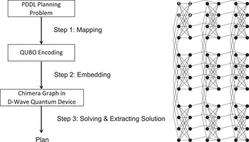
In this paper, we introduce the planning community to the key steps involved in compiling planning problems to QA hardware. Our work is the first to explore the use of QA to solve problems arising in planning and scheduling. This paper is a reworking and deepening of our paper (Rieffel et al., Reference Rieffel, Venturelli, O’Gorman, Do, Prystay and Smelyanskiy2015) to target planning and scheduling researchers, rather than quantum computing researchers. Figure 1 shows the main steps in our framework for solving STRIPS planning problems (Fikes & Nilsson, Reference Ghallab, Nau and Traverso1972; Ghallab et al., 2004) using a D-Wave Two quantum annealer housed at NASA Ames Research Center: mapping the problems to quadratic unconstrained binary optimization (QUBO) and embedding, which takes these hardware-independent QUBOs to other QUBOs that matches the specific QA hardware that will be used.
(Left) The main steps in using quantum annealer to solve an application problem. (Right) A schematic diagram from Smelyanskiy et al., (Reference Smelyanskiy, Rieffel, Knysh, Williams, Johnson, Thom, Macready and Pudenz2012) of the (M, L)-Chimera graph underlying D-Wave’s architecture. In the (3, 4)-Chimera graph shown, there are M 2=9 unit cells, each of which is a fully-connected bipartite graph K 4,4 containing 2L qubits

This work examines different mappings of planning problems to QA, giving insight into their relative strengths and weaknesses. We explore properties of these mappings for a parametrized family of planning problems with a strong scheduling component based on graph coloring (Rieffel et al., Reference Rieffel, Venturelli, Hen, Do and Frank2014), and describe results on the D-Wave Two, enabling a comparison of the performance under these mappings. While the immaturity of the technology means that current results are limited, the significant performance differences that result from different compilation approaches suggest that subtle issues are at play in determining the best compilation approaches for quantum annealers.
2 Ingredients of quantum annealing
QA can be applied to any optimization problem that can be expressed in QUBO. QA is motivated by the possibility that quantum effects such as tunneling allow for efficient exploration of the cost-function landscape in ways unavailable to classical methods.
2.1 Input for quantum annealing: quadratic unconstrained binary optimization problems
QUBO problems are minimization problems with cost functions of the form
 $$q(z_{1} ,\,\ldots{\!},\,z_{N} )\,{\equals}\,{\minus}\mathop{\sum}\limits_{i\,{\equals}\,1}^N h_{i} z_{i} {\plus}\mathop{\sum}\limits_{i\,{\equals}\,1}^{N{\minus}1} \mathop{\sum}\limits_{j\,{\equals}\,i{\plus}1}^N J_{{i,j}} z_{i} z_{j} ,$$
where the z
i
are 0–1 binary variables. A QUBO can be translated to an Ising Hamiltonian, the actual input a quantum annealer takes, through the change of variables
 $$z_{i} \,{\equals}\,{1 \over 2}\left( {s_{i} {\plus}1} \right)$$
.
Before describing the more complex QUBO mappings for general STRIPS planning problems, we give an example of a simple mapping from graph coloring to QUBO.
Example 1. Mapping of Graph Coloring, in which all vertices are to be colored so that any two vertices connected by an edge have different colors, to QUBO. Let G=(V, E) be a graph with n=|V| vertices, where E is the set of edges. The QUBO problem corresponding to the graph coloring problem with k colors on graph G will have kn binary variables, z ic , where z ic =1 means that vertex i is colored with color c, and zic=0 means it is not. The QUBO contains two penalty terms:
 $$\mathop{\sum}\limits_{i\,{\equals}\,1}^n {\left( {1{\minus}\mathop{\sum}\limits_{c\,{\equals}\,1}^k {z_{{ic}} } } \right)^{2} {\plus}\mathop{\sum}\limits_{\left\{ {i,j} \right\} \in E} {\mathop{\sum}\limits_{c\,{\equals}\,1}^k {z_{{ic}} z_{{jc}} } .} } $$
The first corresponds to the constraint that each vertex must be colored by exactly one color:
 $\mathop{\sum}\nolimits_{c\,{\equals}\,1}^k {z_{{ic}} \,{\equals}\,1} $
. The second corresponds to the constraint that two vertices connected by an edge cannot be colored with the same color. For each edge {i, j}, we have a term
 $\mathop{\sum}\nolimits_{c\,{\equals}\,1}^k {z_{{ic}} z_{{jc}} } $
.
2.2 Embedding quadratic unconstrained binary optimizations in specific quantum annealing hardware
As outlined for planning in Figure 1, once an application instance has been mapped to QUBO, a second step is required to compile it to the specific quantum annealing hardware that will be used. Typically, each quantum device has a set of physical quantum bits (qubits) that are linked in a certain way. Ideally, each binary variable z i in a QUBO formula would be represented by a single qubit q i of the machine. Hardware constraints place limits, however, on which qubits can be connected to which other qubits.
The term J i,j z i z j involving qubits q i and q j in the QUBO formula 1 introduced above is physically realized by a coupling between those qubits. D-Wave processors use the Chimera architecture in which each qubit is connected to at most six other qubits (Figure 1), so any QUBO variable that appears in more than six terms must be represented by multiple physical qubits when implemented in this architecture. The D-Wave Two used in the experiments has a (8, 4)-Chimera graph architecture, but with three broken qubits that are not used. Other limitations, beyond the degree six constraint, exist as well. Therefore, each logical qubit must be mapped to a connected set of physical qubits, which, together with the connecting edges, is called the logical qubit’s vertex-model. The overall mapping of logical qubits and couplers to physical ones is called a model, as discussed below.
Consider the simple QUBO z 1 z 2+z 1 z 3+z 2 z 3, which can be graphically represented as a triangle, with the three variables as the vertices and each edge a quadratic term of the QUBO. Ideally, we would represent each variable by a single qubit with hardware connections between each pair so that the QUBO’s three quadratic terms can be directly realized in the hardware. In the hardware graph, Figure 1, no three qubits are all mutually connected to each other. At best, the three variables can be represented by four qubits. We may take, for example, the vertex model for z 1 to be {1, 2}, for z 2 to be {3}, and for z 3 to be {4}, so that there is a connection corresponding to each of the three terms in the QUBO: the term z 1 z 2 can be implemented using the connection between qubits 2 and 3, the term z 1 z 3 between 1 and 4, and the term z 2 z 3 between 3 and 4. The connection between qubits 1 and 2 is also used to encourage the two qubits to take the same value as they are meant to represent a single variable.
3 Mapping general strips planning problems to quadratic unconstrained binary optimization
In this section, we describe two different mappings from a general class of planning problems to QUBO. Specifically, we consider STRIPS planning problems, classical planning problems that are expressed in terms of binary state variables and actions. The first mapping takes a time-slice approach. The second approach first maps a planning problem to SAT, and then reduces higher order terms to quadratic terms through a series of gadgets. Our mappings allow both positive and negative preconditions. Like other compilation approaches that map STRIPS planning problems to substrates such as SAT or MILP, we also bound the compilation horizon to an initial value that is found heuristically. When the corresponding QUBO is not solvable, we gradually extend the horizon until a solution is found.
3.1 Time-slice mapping
This mapping from general classical planning problems to QUBO form is a variant of the one developed and described in (Smelyanskiy et al., Reference Smelyanskiy, Rieffel, Knysh, Williams, Johnson, Thom, Macready and Pudenz2012). This approach shares many similarities with existing compilation approaches (to SAT, CSP, MILP, etc.) derived from the Plan Graph (Blum & Furst, Reference Boros and Hammer1997). Specifically, it presets a horizon L and then encodes the interleaving proposition and action layers up to the preset level L.
If the original planning problem has N state variables x
i
and M actions y
j
, and we are looking for a plan of length L, then we define a time-slice QUBO problem in terms of N(L+1)+LM binary variables. There are two groups of binary variables. The first group consists of N(L+1) binary variables
 $$x_{i}^{{(t)}} $$
that indicate whether the state variable x
i
is 0 or 1 at time step t, for t∈{0, …, L}. The second group consists of LM binary variables
 $$y_{j}^{{(t)}} $$
that indicate whether or not the action y
j
is carried out between time steps t−1 and t. The total cost function is written as a sum:
 $$H\,{\equals}\,H_{{{\rm initial}}} \,{\plus}\,H_{{{\rm goal}}} \,{\plus}\,H_{{{\rm precond}}} \,{\plus}\,H_{{{\rm effects}}} \,{\plus}\,H_{{{\rm no{\minus}op}}} \,{\plus}\,H_{{{\rm conflicts}}} .$$
The first two terms capture the initial condition and the goal condition. Let
 $${\scr I}^{{({\!}{\plus}{\!})}} $$
be the set of state variables that are 1 in the initial condition and
 $${\scr I}^{{({\!}{\minus}{\!})}} $$
be the set of state variables that are initially set to 0. Similarly, let
 $${\cal G}^{{({\!}{\plus}{\!})}} $$
(resp.
 $${\cal G}^{{({\!}{\minus}{\!})}} $$
) be the set of goal variables with value 1 (resp. 0). To capture the requirement that a plan start in the appropriate initial state and meets the goals, we include in the cost function the term
 $$H_{{{\rm initial}}} \,{\equals}\,\mathop{\sum}\limits_{i\, \in\, {\scr I}^{{\left( {\!}{\plus}{\!} \right)}} } \left( {1{\minus}x_{i}^{{\left( 0 \right)}} } \right){\plus}\mathop{\sum}\limits_{i\, \in \,{\scr I}^{{\left( {\!}{\minus}{\!} \right)}} } x_{i}^{{\left( 0 \right)}} ,\quad H_{{{\rm goal}}} \,{\equals}\mathop{\sum}\limits_{i \,\in\, {\cal G}^{{\left( {\!}{\plus} \right{\!}{\!})}} } \left( {1{\minus}x_{i}^{{\left( L \right)}} } \right){\plus}\mathop{\sum}\limits_{i \,\in\, {\cal G}^{{\left( {\!}{\minus}{\!} \right)}} } x_{i}^{{\left( L \right)}}. $$
We next add terms to the cost function that penalize a plan if an action is placed at time t, but the prior state does not have the appropriate preconditions:
 $$H_{{{\rm precond}}} \,{\equals}\,\mathop{\sum}\limits_{t\,{\equals}\,1}^L \mathop{\sum}\limits_{j\,{\equals}\,1}^M \left( {\mathop{\sum}\limits_{i\, \in\, {\cal C}_{j}^{{\left( {\!}{\plus}{\!} \right)}} } \left( {1{\minus}x_{i}^{{\left( {t{\minus}1} \right)}} } \right)y_{j}^{{\left( t \right)}} } \right.{\plus}\left. {\mathop{\sum}\limits_{i \,\in\, C_{j}^{{\left( {\!}{\minus} \right{\!})}} } x_{i}^{{\left( {t{\minus}1} \right)}} y_{j}^{{\left( t \right)}} } \right),$$
where
 $${\cal C}_{j}^{{({\!}{\plus}{\!})}} $$
is the set of positive preconditions for action j and
 $${\cal C}_{j}^{{({\!}{\minus}{\!})}} $$
is the set of negative preconditions. Next, we must penalize variable changes that are not the result of an action. We start with this term, the H
no--op term, that penalizes variable changes:
 $$H_{{{\rm no{\minus}op}}} \,{\equals}\,\mathop{\sum}\limits_{t{\equals}1}^L \mathop{\sum}\limits_{i\,{\equals}\,1}^N \left[ {x_{i}^{{\left( {t\,{\minus}\,1} \right)}} {\plus}x_{i}^{{\left( t \right)}} {\minus}2x_{i}^{{\left( {t{\minus}1} \right)}} x_{i}^{{\left( t \right)}} } \right].$$
This term gives a cost penalty of 1 every time a variable is flipped. Of course, when the effect of an action does result in a variable flipping, we do not want this penalty, so we will make up for this penalty when we add the term that corresponds to the effects of an action. Specifically, we need to penalize if the subsequent state does not reflect the effects of a given action. Let
 $${\epsilon}_{j}^{{({\!}{\plus}{\!})}} $$
be the set of positive effects for action j and
 $${\epsilon}_{j}^{{({\!}{\minus}{\!})}} $$
the set of negative effects. The penalty if the appropriate effects do not follow the actions is captured by the following term:
 $$H_{{{\rm effects}}} \,{\equals}\,\mathop{\sum}\limits_{t\,{\equals}\,1}^L \mathop{\sum}\limits_{j\,{\equals}\,1}^M \left( {\mathop{\sum}\limits_{i \,\in\, {\epsilon}_{j}^{{\left( {\!}{\plus} \right{\!})}} } y_{j}^{{\left( t \right)}} \left( {1{\plus}x_{i}^{{\left( {t{\minus}1} \right)}} {\minus}2x_{i}^{{\left( t \right)}} } \right)} \right.{\plus}\left. {\mathop{\sum}\limits_{i \,\in \,{\epsilon}_{j}^{{\left( {\!}{\minus} \right{\!})}} } y_{j}^{{\left( t \right)}} \left( {2x_{i}^{{\left( t \right)}} {\minus}x_{i}^{{\left( {t{\minus}1} \right)}} } \right)} \right).$$
In order to understand this term, we must consider it together with the no-op term. When
 $$y_{j}^{{\left( t \right)}} {\equals}1$$
, the corresponding term for
 $$i\in{\epsilon}_{j}^{{\left( {\!}{\plus} \right{\!})}} $$
(resp.
 $$i\in{\epsilon}_{j}^{{\left( {\!}{\minus} \right{\!})}} $$
), taken together with the no-op term, can be written
 $$\left( {1{\plus}2x_{i}^{{\left( {t{\minus}1} \right)}} } \right)\left( {1{\minus}x_{i}^{{\left( t \right)}} } \right)$$
(resp.
 $$\left( {3{\minus}2x_{i}^{{\left( {t{\minus}1} \right)}} } \right)x_{i}^{{\left( t \right)}} $$
for negative effects), resulting in a positive penalty unless
 $$x_{i}^{{\left( t \right)}} {\equals}1$$
(resp.
 $$x_{i}^{{\left( t \right)}} {\equals}0$$
). By using this form we have corrected for the corresponding no-op term.
3.1.1 Parallel plans
Classical planners often allow for parallel plans in which more than one action can take place at one time if those actions could have been done in any order. Encodings that allow parallel plans are often significantly smaller due to the big reduction in the preset horizon value L. The QUBO encoding described so far works fine for domain with linear plans, but when more than one action can take place at a given time, we are in danger of over-correcting for the no-op term. If multiple actions at the same time have the same effect, the H effects term will add a term for each of those actions, thus overcompensating for the no-op penalty. To avoid overcompensating, we penalize multiple actions at the same time having the same effect, discouraging all such actions to ensure that two actions that conflict in the sense that positive preconditions of one overlap with negative effects of the other or vice versa, and to avoid overcompensating, we include the penalty:
 $$H_{{{\rm conflict}}} \,{\equals}\,\mathop{\sum}\limits_{t\,{\equals}\,1}^L \mathop{\sum}\limits_{i\,{\equals}\,1}^N \left( {\mathop{\sum}\limits_{\left\{ {j\,\mid\,i\in{\cal C}_{j}^{{\left({\!} {\plus} \right{\!})}} {\cup}{\epsilon}_{j}^{{\left( {\minus} \right{\!})}} } \right\}} \mathop{\sum}\limits_{\left\{ {j'\,\ne\,j\,\mid\,i\in{\epsilon}_{{j'}}^{{\left({\!} {\minus} \right{\!})}} } \right\}} y_{j}^{{\left( t \right)}} y_{{j'}}^{{\left( t \right)}} } \right.{\plus}\left. {\mathop{\sum}\limits_{\left\{ {j\,\mid\,i\in{\cal C}_{j}^{{\left({\!} {\minus} \right{\!})}} {\cup}{\epsilon}_{j}^{{\left( {\!}{\plus} \right{\!})}} } \right\}} \mathop{\sum}\limits_{\left\{ {j'\,\ne\,j\,\mid\,i\in{\epsilon}_{{j'}}^{{\left( {\plus} \right)}} } \right\}} y_{j}^{{\left( t \right)}} y_{{j'}}^{{\left( t \right)}} } \right).$$
3.1.2 Encoding size improvements
Although for explanatory purposes it was useful to include variables for the state at time t=0, those specified by initial conditions can be set ahead of time, so that we don’t need to include the H
initial term. The same is true of the H
goal term. We can also replace all of their occurrences in H
no--op, H
precond, and H
effect with these set values to simplify those constraints. Furthermore, reachability and relevant analysis starting from the initial and goal states, preprocessing techniques employed by compilation-based planners such as Blackbox (Kautz & Selman, Reference Kautz and Selman1999) and GP-CSP (Do & Kambhampati, Reference Dubois and Mandler2001), can be used to remove or preset the values of variables in different layers. These simplifications result in modified terms H′no--op, H′precond, and H′effects. In addition, as in our setting we have followed the convention that preconditions must be positive, we can use a simpler version of the H
precond term:
 $$H'_{{{\rm precond}}} \,{\equals}\,\mathop{\sum}\nolimits_{t\,{\equals}\,1}^L \mathop{\sum}\nolimits_{j\,{\equals}\,1}^M \mathop{\sum}\nolimits_{i\in{\cal C}_{j}^{{\left( {\!}{\plus} \right{\!})}} } \left( {1{\minus}x_{i}^{{\left( {t{\minus}1} \right)}} } \right)y_{j}^{{\left( t \right)}} .$$
For the scheduling problems we consider here, the QUBO simplifies to
 $$H\,{\equals}\,H_{{{\rm no{\minus}op}}}^{{\rm '}} {\plus}H_{{{\rm precond}}}^{'} {\plus}H_{{{\rm effacts}}} {\plus}H_{{{\rm conflict}}} .$$
3.2 Conjunctive normal form-based mapping
We also explored first mapping planning problems to SAT (in conjunctive normal form (CNF) form) and then using a standard approach to map the resulting CNF expression to QUBO. A SAT’s CNF expression over n Boolean variables {x i } consists of a set of clauses {C a }, each with k variables, possibly negated, connected by logical ORs: b 1∨b 2∨, …, ∨b k , where b i ∈{x 1, x 2, …, x n , ¬x 1, ¬x 2, … , ¬x n }. The number of variables k in the clause can vary from clause to clause. The clauses are connected by an AND operator, meaning all of the clauses must be satisfied.
We used the first of four PDDL-to-CNF translators built into the SATPLAN planner (Kautz, Reference Kautz2004). This “action-based” encoding starts with a time-slice encoding approach and then further removes all variables representing state variables while adding constraints that capture the relationships between actions in consecutive time steps that were previously enforced by relationships between actions and state variables. We chose this encoding because it tends to produce the smallest SAT encodings, which are more likely to translate to QUBOs that embed in the current D-Wave machine hardware.
To convert a CNF instance to QUBO, we first transform it to a polynomial unconstrained binary optimization (PUBO), a generalization of QUBO, which allows terms with higher than quadratic degree. Each clause of a CNF instance translates to a PUBO instance that is the conjunction of the negation of all the literals in that clause; a negative literal is replaced by a binary variable and a positive literal is replaced by the difference of 1 and the corresponding binary variable. For example, the CNF clause (x 1∨¬x 2∨¬x 3∨x 4) would correspond to the PUBO term (1−x 1)x 2 x 3(1−x 4).
We reduce higher degree terms in a PUBO to quadratic using an iterative greedy algorithm related to one described in (Boros & Hammer, Reference Cai, Macready and Roy2002). At each step, a pair of variables that appears in most terms is replaced by an ancilla variable corresponding to their conjunction. We add a penalty term to ensure the ancilla variable corresponds to this conjunction. For example, for the term x 1 x 2 x 3, we may introduce an ancilla variable y 12 to replace x 1 x 2, and add a penalty term 3y 12+x 1 x 2−2x 1 y 12−2x 2 y 12, which is 0 if y 12=x 1 x 2 and >0 otherwise. We remove the term x 1 x 2 x 3 from the PUBO, replacing it with y 12 x 3+3y 12+x 1 x 2−2x 1 y 12−2x 2 y 12. We use a penalty weight greater by 1 than the sums of the magnitudes of the positive and negative coefficients of the terms the ancilla is used to reduce (Babbush et al., Reference Blum and Furst2013) to ensure that the constraint-satisfying solutions have lower total cost than the constraint-violating solutions. This procedure is repeated until the resulting PUBO is quadratic.
4 Experimental setup
Many planning applications include scheduling aspects (Chien et al., Reference Coja-Oghlan2012). Scheduling, which deals with assigning resources and time to tasks while taking into account constraints, is in itself an important problem. Certain classes of scheduling problems correspond to graph coloring. For example, a scheduling problem with a set of tasks and constraints such that any pair of tasks competing for the same resource cannot be assigned the same time-slot can be phrased as vertex coloring, a well-known NP-complete problem. Specifically, the chromatic number (the smallest number of colors needed) represents the smallest number of time-slots needed to complete a corresponding schedule, thus representing the minimum makespan.
To evaluate our approach, we use a benchmark set of planning instances based on graph coloring (Rieffel et al., Reference Rieffel, Venturelli, Hen, Do and Frank2014) that consist of parametrized families of hard planning problems. Having parametrized families enables the investigation of scaling behavior using small problems, which is crucial for evaluating early technology that is not mature enough to run real-world problems. Because of the overhead in mapping and embedding planning problems, even the smallest IPC problems (International Planning Competition, Reference Achlioptas and Friedgut2004) are more than an order of magnitude too large to be run on the current D-Wave device.
4.1 Vertex coloring as planning
A scheduling problem in which no pair of tasks can be assigned the same time-slot is analogous to a coloring instance in which the tasks are vertices, conflicts are edges, and the minimum makespan is the chromatic number, which is the minimum number of colors necessary to color each of the vertices such that no two adjacent ones have the same color. Given an undirected graph G={V, E} with n vertices and k colors, the vertex coloring problem asks for a solution in which (1) all vertices are colored and (2) any pair of vertices connected by an edge is colored differently. The corresponding planning problem is as follows: for each vertex v there are
-
∙ k actions
 $$a_{v}^{c} $$
representing coloring v with color c,
-
∙ A “goal variable”
$$s_{v}^{g} $$
representing whether or not v has been colored at all, and -
∙ A “state variable”
$s_{v}^{c} $
representing whether or not v has been colored with the color c.


Let C(v) be the set of neighboring vertices that are connected to v by an edge. For each action
 $a_{v}^{c} $
, there are |C(υ)|+1 preconditions:
 $\left( 1 \right)s_{v}^{g} \,{\equals}\,F$
, indicating that v is not already colored; and (2) for each
 $w \in C (v), \ s_{w}^{c} \,{\equals}\,F$
, guaranteeing that none of neighboring vertices are already colored with color c. Each action
 $a_{v}^{c} $
has two effects:
 $s_{v}^{g} \,{\equals}\,T$
and
 $s_{v}^{c} \,{\equals}\,T$
. In the initial state, none of the vertices are colored:
 $$\forall v\inV,\,\forall c\in\left[ k \right]\,\colon\,\,s_{v}^{g} \,{\equals}\,F$$
, and
 $s_{v}^{c} \,{\equals}\,F$
. The goal state requires that all vertices are colored:
 $\forall v\inV\,\colon\,\,s_{v}^{g} \,{\equals}\,T$
. A plan is a sequence of n actions, each of which colors a vertex v.
4.1.1 Problem generation
We parametrically generate instances using the Erdös-Rényi model of random graphs G n,p , where n is the number of vertices and p is the probability of an edge between each pair of vertices, using an extension of Culberson et al.’s (Reference Das and Chakrabarti1995) graph generator program. Our extension generates PDDL files (Rieffel et al., Reference Rieffel, Venturelli, O’Gorman, Do, Prystay and Smelyanskiy2015), at the phase transition c=pn=4.5 (Achlioptas & Friedgut, Reference Achlioptas and Moore1999; Dubois & Mandler, Reference Farhi, Goldstone, Gutmann and Sipser2002; Achlioptas & Moore, Reference Babbush, O’Gorman and Aspuru-Guzik2003; Coja-Oghlan, Reference Culberson, Beacham and Papp2013). We preset the number of colors to k=3 and for that k value the maximum problem size that we can embed in the D-Wave Two machine with 509 qubits is n=16. For each of n=8, 9, …, 16, we use 100 solvable problem instances at the phase transition for each size. For each generated instance, we then generate three different QUBOs, each described in the previous sections: (i) direct mapping; (ii) time-slice mapping; and (iii) CNF-based mapping.
4.1.2 Embedding
From a mapped QUBO instance, we generate a vertex model by running D-Wave’s heuristic embedding software (Cai et al., Reference Chien, Johnston, Frank, Giuliano, Kavelaars, Lenzen, Policella and Verfailie2014) on the mapped QUBO instance, using the software’s default parameters. The output of the embedding software is a set of pairwise-disjoint, connected vertex models {C i } in the hardware graph corresponding to the variables {z i } in the original QUBO, which will then be converted to Ising form to be run on the D-Wave machine. Before running, the Ising is rescaled so that all coefficients are between [−1, 1]. We performed our own parameter setting following (Rieffel et al., Reference Rieffel, Venturelli, O’Gorman, Do, Prystay and Smelyanskiy2015), rather than using D-Wave’s defaults.
4.1.3 Solving
All quantum annealing runs were on the 509-qubit D-Wave Two machine housed at NASA Ames with an anneal time of 20 microseconds. For each embedded QUBO instance, we performed 450,000 anneals for 10 gauges (i.e. local symmetry transformations that leave the objective function invariant but reduce the effect of hardware biases(Perdomo-Ortiz et al., Reference Perdomo-Ortiz, Fluegemann, Biswas and Smelyanskiy2015)), for a total of 450 000 anneals per instance.
We consider only solvable instances, so that the minimum value of all our QUBO instances is zero. For each embedded instance, once we obtain the 450,000 results from the run, we check how many times the minimal value was obtained, which gives us the probability of solution r. We then compute the expected number of runs
 $R{\equals}{{\ln \left( {1{\minus}0.99} \right)} \over {\ln \left( {1{\minus}r} \right)}}$
required to obtain a 99% success probability, multiplied by the anneal time of 20 microseconds, and report 20×R microseconds, the expected total anneal time to 99% success probability. We are effectively using a 0.9 seconds cutoff time as the expected anneal time when only one anneal solves is 0.9 seconds. Given that classical planners solve these problems in <0.1 seconds, with the best planners for these problems solving them in <0.01 seconds (Rieffel et al., Reference Rieffel, Venturelli, Hen, Do and Frank2014), this cutoff time seems reasonable.
We report the median expected total anneal time across 100 instances, with error bars corresponding to the 35th and 65th percentiles. Each data point shown therefore represents 45 million anneals. Although the total annealing time for each point is only 90 seconds, because the process to read-out the state of all qubits (i.e. solution extraction) takes considerably longer than the anneal time, and because of shared use of the machine, the wall clock time to obtain a single data point is hours rather than minutes. Finding the embedding, by far the longest step in the process, can take minutes for the largest instances, but fortunately needs to be performed only once per QUBO instance.
5 Results and analysis
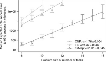
Figure 2 shows the relative performance, in terms of median expected total annealing time for 99% success, of the D-Wave Two on the family of graph coloring-based planning problems described above. When at least half of the instances do not solve within the 0.9 seconds effective cutoff time, we no longer show the point. For the CNF mapping, that happens by problem size 11, and for the time-slice instances by problem size 13. The figure also shows the performance using a direct map of graph coloring to QUBO. As expected, this direct mapping performs better than both general mappings for planning problems as it is more compact.
Comparison of the median expected total anneal time to 99% success for the two mappings. Each data point shows the median expected total annealing time to achieve 99% success over the 100 problems of each size given on the x-axis. The error bars are at the 35th and 65th percentiles. When at least half of the instances do not solve within the 0.9 seconds effective cutoff time, we no longer show the point. Also, when fewer than 65% solve, the top of the error bar is indeterminate, as happened for the last point shown in both the conjunctive normal form (CNF) and time-slice (TS) series

There is a substantial difference between the performance on the time-slice instances and the CNF instances, with the median expected total annealing time to achieve 99% success being about a factor of 5 greater for the CNF instances than for the time-slice instances (Figure 2). The scaling for the time-slice approach is also significantly better than for the CNF approach, with an α-value of 1.37 rather than 1.76 (though the scaling is estimated on very few data points). Rieffel et al., (Reference Rieffel, Venturelli, O’Gorman, Do, Prystay and Smelyanskiy2015) compared several properties of both the mapped and embedded QUBOs for the two mappings, but these simple properties were all sufficiently similar across the two mappings that they could not account for so marked a difference in performance.
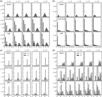
We took a deeper look at the distributions of various simple properties related to the mapped and embedding QUBOs arising from the two mappings. We also show the distributions for the direct map for comparison. In the mapped QUBOs, we looked at the distribution of of vertex degrees (the number of quadratic terms in which a variable z i appears in the mapped QUBO). As can be seen in Figure 3a, the histograms for the time-slice and CNF mappings are very similar, whereas they differ markedly from the histograms for the direct map. In the embedded QUBOs, we looked at the distribution of the vertex model sizes (Figure 3b), and also the distribution of the graph diameter of the vertex models (not shown), but found little difference between the distributions for the time-slice and CNF embedded QUBOs. Therefore these properties can contribute at most a small amount to the performance difference between the two mappings.
Analysis and comparison of mapped and embedded Quadratic Unconstrained Binary Optimization (QUBO) features for each problem size under three mappings: direct mapping, time-slice mapping, and conjunctive normal form (CNF) mapping (a) Vertex degree histogram. Histograms of the vertex degrees for the mapped QUBO graphs. (b) Vertex model size histogram. Histograms of the vertex model sizes in the embedded QUBOs. (c) QUBO coefficient histogram. Histograms of the h i and J ij in the mapped QUBOs. (d) Histogram of h i and j i =Σ j J ij . Histograms of the h i and j i =Σ j J ij in the mapped QUBOs.

We begin to see differences when we look at distributions of the coefficients in the mapped QUBOs. Figure 3c shows histograms of the coefficient of the mapped QUBOs (Equation (1)), converted to Ising, and rescaled so that all of the h i and J ij coefficients are between [−1, 1]. Let j i =∑ j J ij . Figure 3d shows a histogram of the h i and j i . Both histograms show significant differences between the two mappings.
Another potential origin of the performance difference is the topology of the vertex models. A quick analysis showed that for all three mappings nearly all (>99%) of the vertex models of the embedded QUBOs are trees. A further classification of the graph structures, and their relative frequencies, could potentially lead to greater insight.
6 Conclusions and future work
We show how quantum annealing can solve planning problems via mapping to QUBO. We introduced two general mapping techniques and applied them to planning problems based on graph coloring. We ran these problems on an early quantum annealer and saw significant performance differences. We began an investigation of various properties of the mapped and embedded QUBOs to understand which properties do and do not contribute to the performance differences.
One of the biggest open questions in quantum computing is the breadth of its applications. Although certain quantum algorithms have been proven to outperform classical algorithms on classes of problems of practical interest, the potential advantage of quantum methods for the vast majority of problems remains unexplored. Many of the most useful classical algorithms in use today are heuristic algorithms, which have not been mathematically proven to outperform other approaches, but have been shown to be more effective empirically. Only recently, with the advent of early quantum annealers, could empirical investigation of quantum techniques begin. Major hardware development efforts are underway to build better quantum computational hardware. In order to fully explore the potential of this hardware, we must understand how best to compile practical problems to a form that is suitable for quantum hardware. Early quantum annealing hardware can handle only small instances. At this early stage there is no advantage in solving STRIPS planning problems via quantum annealing over classical compilation approaches such as SAT, CSP, or MILP. Nevertheless, by analyzing the results obtained under these limitations, we can gain insights into the best programming and compilation techniques for quantum annealers, and ultimately into the potential of quantum annealing to solve problems of practical interest in planning and scheduling and beyond.
Acknowledgments
The authors are grateful to Zhihui Wang for helpful discussions. This work was supported in part by the Office of the Director of National Intelligence (ODNI), the Intelligence Advanced Research Projects Activity (IARPA), via IAA 145483; by the AFRL Information Directorate under grant F4HBKC4162G001. The views and conclusions contained herein are those of the authors and should not be interpreted as necessarily representing the official policies or endorsements, either expressed or implied, of ODNI, IARPA, AFRL, or the US Government. The US Government is authorized to reproduce and distribute reprints for Governmental purpose notwithstanding any copyright annotation thereon. The authors also like to acknowledge support from the NASA Advanced Exploration Systems program and NASA Ames Research Center and NASA grant NNX12AK33A.