From late 1933 to May 1935 American industrial policy promoted cartels and industrial planning as a method of spurring recovery. The ostensible goal of the National Industrial Recovery Act of 1933 (NIRA) was to “eliminate cutthroat competition” and promote “fair competition.” In consultation with government officials, industry leaders drafted codes of conduct to regulate competitive behavior. The question of whether the NIRA was successful in facilitating collusion, as well as whether any such success was positive for the economy, has been debated to the present.
We use plant-level records from the Census of Manufactures in 1929, 1931, 1933, and 1935 to study collusion under the NIRA. This article examines the macaroni industry, which was the focus of Barbara Alexander (Reference Alexander1997). She models the difficulties of sustaining collusion even in the case in which the government actively encourages, though does not mandate, such behavior. She argues that cost differences among producers were too large to permit agreement on how to divide the market.
The macaroni industry had several attractive characteristics for studying collusion under the NIRA, as Alexander notes. It is unconcentrated and actually experienced a decline in profits while the NIRA was in force. Moreover, the product is income inelastic, helping to minimize the effects of macroeconomic conditions on measures of performance. For these reasons, testing for collusion in this industry provides a “lower bound” on the prevalence of anti-competitive behavior under these codes. Insofar as we find evidence for dampening of competition in this industry, then it is likely to be present in a wide variety of industries.
Joseph Harrington (Reference Harrington and Buccirossi2008) summarizes the literature on screening for collusive conduct. These screens are empirical tests that are relatively insensitive to the exact modeling specifications of the industry. In Harrington's words, screening provides a way to “triage” industries for further study. We apply this screening approach in this article. There are many such screens, some as basic as changes in price-cost margins. As noted by Alexander (Reference Alexander1997), the macaroni industry would not look collusive under this test, with margins essentially unchanged after the NIRA comes into force. Rather than focus on price-cost margins, we look for three other markers of plant pricing behavior. In particular, we examine changes in the following statistics: (1) cost pass-through, (2) cross-sectional dispersion in prices, and (3) time-series persistence in prices. We emphasize that these screens are less sensitive to being driven by aggregate shocks, lessening though not eliminating the worry inherent in using only time variation to identify shifts.
Declines in all of these statistics can be jointly rationalized as the outcome of a dynamic pricing game with private information about cost, as in Susan Athey and Kyle Bagwell (Reference Athey and Bagwell2008). However, our results are not constrained to this setup, as collusion, implicit or otherwise, causes plants to become less responsive to cost shocks.Footnote 1 This connection is a standard intuition in industrial organization stretching back to Frederick Mills (Reference Mills1927). The simplest models in which to see this result are perfect competition versus monopoly. Under perfect competition, all of a change in common costs is passed through into prices. In contrast, pass-through is less than complete under monopoly. Because prices are less sensitive to cost shocks after an increase in cartelization, collusion leads to lower variance in prices both within a plant over time and between plants in the cross-section. Other studies have used dispersion in prices as evidence for collusion. Both Yuliya Bolotova, John Connor, and Douglas Miller (Reference Yuliya, Connor and Miller2008) and Rosa Abrantes-Metz et al. (Reference Abrantes-Metz, Froeb, Geweke and Taylor2006) compare the variance of prices before and after known cartels were broken up and find large increases in the variance after the cartel is eliminated. Finally, because prices are less dispersed under collusion, the time series persistence of prices is lower. While this type of test is implied by the model of Athey and Bagwell (Reference Athey and Bagwell2008), we are aware of no empirical implementations of it.
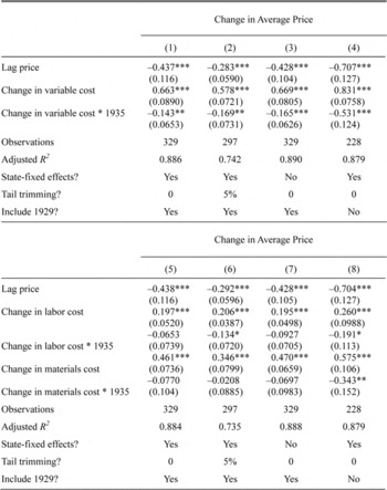
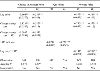
We find that a 1 percent change in variable cost translates into 0.66 percent increase in price before the NIRA. That same change leads to only a 0.52 percent increase while the NIRA is in effect, a reduction of one-fifth. This effect is robust to a variety of specifications that make different assumptions about the informativeness of outlier observations and the inclusion of certain fixed effects. We then examine to what extent the pass-through of different components of cost change after the NIRA is introduced. Competitive pricing implies that the pass-through of a particular component should be equal to its share in marginal cost. In a noncompetitive model with perfect information, changes in costs should be passed through in relation to their share of the inputs, but this need not be the case if observation of the information about the different costs differs. In percentage terms, we find a larger decline in the pass-through of shocks to labor costs than that for materials costs after the NIRA.
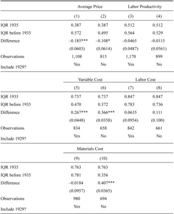
There is a decline during the NIRA period in the dispersion of prices as measured by the interquartile range (IQR). After the NIRA was introduced, the IQR falls by about one-fifth in our most conservative specification and just under one-third in our preferred specification.Footnote 2 The autocorrelation of prices is reduced by about 30 percent after the NIRA is introduced. None of the cost components shows a statistically significant decline in their persistence.
Finally, we consider the results across two different groups of plants: incorporated and unincorporated. The code governing competitive behavior was drafted in consultation between the manufacturers trade group and the government. While we do not have direct evidence on which firms were most successful in influencing the rules chosen, it seems plausible that incorporated firms rather than small, unincorporated operations shaped the rules in their interests. Under this conjecture, one would expect to find incorporated firms to have a larger response to the introduction of the NIRA than unincorporated firms, which have an incentive to deviate from rules less tailored to their situation. We confirm such a difference in the data. All three of our tests show much larger changes in the behavior of incorporated plants, although the effects are present in both groups. This exercise helps to address the issue that almost all of our identifying variation comes from structural breaks in the time series with no “control” group. By using this cross-sectional variation, we provide an additional approach to identifying collusion by comparing the behavior of plants that are ex ante more likely to be engaged in anti-competitive behavior.
The literature has been divided on the micro-level effects of these codes. Alexander (Reference Alexander1994) finds that the “critical concentration ratio” for collusion falls after the introduction of the NIRA, which she takes as evidence that the codes facilitated collusion.Footnote 3 One issue with this study is that the concentration ratio only exists for a limited set of industries, as noted by Matthew Krepps (Reference Krepps1997). Jason Taylor (Reference Taylor2002) finds that output falls after the codes come into force, which is consistent with a cartelization story. In subsequent work, Taylor (Reference Taylor2007) identifies particular features of the codes that were helpful in sustaining collusion. Finally, Mark Chicu, Vickers, and Ziebarth (Reference Chicu, Vickers and Ziebarth2013) study the cement industry using the same census source. In that work, they develop a spatial model of competition tailored to the industry and develop a test for collusion derived from it. The evidence for that industry is in favor of the NIRA having increased collusive behavior.
Others have suggested that these codes had limited effects on promoting collusion. Alexander (Reference Alexander1997), Krepps (Reference Krepps1997), and Alexander and Gary Libecap (Reference Alexander and Libecap2000) all argue that a nudge from the government was not enough to induce collusion. In this view, the penalties to violating the code agreement, such as the loss of the right to use the Blue Eagle emblem, were not sufficiently severe to allow collusion.Footnote 4 Alexander suggests that the reason for the failure of the codes, at least in her particular example of the macaroni industry, is because of intra-industry heterogeneity. These differences create tension between low and high cost producers over the optimal price, and small shifts in exogenous circumstances can push low cost plants to exploit their advantage and undercut the agreement. The problem with testing this interpretation from an empirical standpoint is that Alexander has no data on heterogeneity at the plant level, so she relies on mainly narrative evidence. Both Ellis Hawley (Reference Hawley1974) and Donald Brand (Reference Brand1988) make similar arguments regarding the sources of conflict within industries, with the added contention that these codes were drawn up to benefit small plants. More recent work by Alexander and Libecap (Reference Alexander and Libecap2000) uses some limited plant-level data to look for heterogeneity in costs. They too argue that because of these production differences, plants were not able to collude despite being given an opportunity. Responding to Alexander (Reference Alexander1994), Krepps (Reference Krepps1997) finds no evidence that the critical concentration ratio actually changed once a consistent set of industries are used. Pamela Pennock (Reference Pennock1997) studies the tire industry and finds that the NIRA code actually served to create discord between producers rather than promoting coordination. Finally, George Bittlingmayer (Reference Bittlingmayer, McChesney and Shughar1995) argues that while the codes worked in generating collusion, they actually promoted efficiency in industries with large fixed costs.
HISTORICAL BACKGROUND
The year 1933 was the nadir of the Great Depression. Real GDP and industrial production both bottomed out in this year, and unemployment reached its peak. That year also saw major reforms pushed by newly elected President Franklin Roosevelt, who thought that the Depression was caused by excess competition. As cited in Arthur Schlesinger (Reference Schlesinger2003), Roosevelt said in an early campaign speech that, “Competition has been shown to be useful up to a certain point and no further, but cooperation, which is the thing we must strive for today, begins where competition leaves off.” Roosevelt argued that price cutting drove out businesses, leading to deflation and low wages which ultimately resulted in underconsumption. The proposed solution was greater national planning and coordination within industries through trade associations, with a focus on reflation. As cited in Gaudi Eggertsson (Reference Eggertsson2012), Roosevelt said on May 1, 1933: “We are agreed in that our primary need is to insure an increase in the general level of commodity prices. To this end simultaneous actions must be taken both in the economic [i.e., the NIRA] and the monetary fields.”
In May 1933 the National Industrial Recovery Act was drafted to promote cooperation through “Codes of Fair Competition.” It was quickly approved by the House but was delayed in the Senate over a clause to protect the collective bargaining rights of workers. Eventually, the bill was signed into law by Roosevelt on June 16. By the end of 1933 a large number of codes for major industries had already been drawn up and approved by the administration. In addition, hundreds of other industries were seeking approval of codes they had submitted. The codes were supposed to be formulated as a collaborative process between industry, labor, and the consumer. The latter two had explicit representatives appointed by the government, while a particular industry was usually represented by its trade association. In reality, the consumer advocate had little effect and the labor representative was a government official who was usually satisfied with an agreement if it contained a collective bargaining provision (Hawley Reference Hawley1974). Although the code in the macaroni industry was not approved until 1934, anecdotal evidence in other industries suggests that some collusive activity began subsequent to the passage of the law but prior to ratification of the code (Chicu, Vickers, and Ziebarth Reference Chicu, Vickers and Ziebarth2013). In our tests, we generally treat 1933 as not under the NIRA, but show robustness checks classifying 1933 as under the regime.
While it was intended that codes be ratified by a one-plant-one- vote system, the process of drafting the code was usually controlled by the largest plants, which tended to dominate the trade associations. For example, in the cement industry, the trade association that drew up the code originally consisted of about ten firms before a large group of firms joined almost coincidentally with the introduction of the NIRA (Chicu, Vickers, and Ziebarth Reference Chicu, Vickers and Ziebarth2013). At the same time, the process was not free of conflict, and questions still exist about who exactly the codes were supposed to benefit. Both Hawley (Reference Hawley1974) and Brand (Reference Brand1988) thought the codes were drawn up to benefit the smallest, high-cost producers in an industry.
The codes did have some common components across industries. Collective bargaining with labor was required of all codes. Many codes had minimum price rules that forbade selling output below “cost,” where the definition of cost was somewhat varied across different codes. Others had minimum wage regulations that varied across different regions of the country. Some even had explicit output quotas. There were explicit punishments by the government if a firm violated the code, including possible jail time. A division was setup to ensure compliance, and before early 1934, those who complied could display the Blue Eagle, a coveted symbol by businesses (Klein and Taylor Reference Klein and Taylor2008).
At the same time, there are questions about the direct costs of following or not following the code. First, there were limitations to the effectiveness of this explicit enforcement by the government. Very few firms were ever actually punished. Second, firms worried about the potential costs from antitrust suits if they followed explicitly anti-competitive codes.Footnote 5 To provide some clarity on this matter, some states passed laws explicitly exempting firms operating under the codes from antitrust prosecution under state law (Chicu, Vickers, and Ziebarth Reference Chicu, Vickers and Ziebarth2013). Overall, these codes if followed strictly would have circumscribed competitive behavior and created radical changes in the relationship between business and employee, business and customer, and business and government.
On May 27, 1935 the Supreme Court handed down a unanimous decision invalidating the major provisions of the NIRA in the Schechter case. Central to the decision was the conclusion that the act unconstitutionally delegated too much power to the executive branch in allowing the president to set up and enforce the codes of fair competition. While the case has received much attention, many have argued that Congress was unlikely to have renewed the act anyway, so the court only hastened its demise. Even though the act was invalidated, authors such as Harold Cole and Lee Ohanian (Reference Cole and Lee2004) suggest that the repeal had little practical impact on antitrust enforcement as the Roosevelt administration continued to decline to enforce existing antitrust laws. By 1938 Roosevelt was strongly antimonopoly, going so far as to suggest antitrust enforcement was necessary to prevent the United States from becoming a “fascist-collective” (Freyer Reference Freyer2006, p. 8).
DATA AND INDUSTRY BACKGROUND DATA
The data used for this article come from the Census of Manufactures (CoM) collected by the Census Bureau in various forms since 1810.
COMPARISON OF INDIVIDUAL SCHEDULES FROM NATIONAL ARCHIVES TO PUBLISHED CENSUS RETURNS

Note:
The National Archive totals for 1931 include schedules excluded from published census returns because the establishment filed a schedule but was below the cutoff set by the census.
Source:
Authors' calculations are from the Census of Manufacturers, 1929–1935. See the text for details.
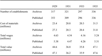
Though many years of schedules of the manufacturing censuses have been lost, the schedules for 1929, 1931, 1933, and 1935, the first half of the Great Depression, were kept and are housed at the National Archives.Footnote 6 The schedules provide detailed information on labor, materials, and output. The biggest issue when working with this data is coverage. First, there is the question of whether all the schedules collected by the Census are at the Archives. In Table 1, we compare the schedules we have collected to the totals published by the Census Bureau. For the latter three censuses, the results are very similar, suggesting that the amount of missing data from the Archives is small, leaving aside the issue of whether plants were actually counted. In 1929 there do appear to be a number of schedules missing. For this reason, we exclude 1929 from some of our specifications. The second question about the quality of the data is how well the census was conducted. Unfortunately, we know of no extant industry-level data sources to check the consistency of the census data for macaroni. Other studies noted in Nicolas Ziebarth (Reference Ziebarth2013) have found very good coverage for other industries with outside sources of validation.
INDUSTRY AND CODE BACKGROUND
The following discussion regarding the macaroni industry follows Alexander (Reference Alexander1997). The macaroni industry includes all kinds of dried pasta, from spaghetti to egg noodles. The industry was mainly concentrated in a few states, in particular New York and California. Alexander argues that the industry contained three main types of producers: small family-owned operations that sold locally, large industrial concerns that shipped nationally, and a middle tier of regional producers. The bigger plants used large-scale production processes that made them much more efficient than the small producers. As Alexander points out, this created a major disparity in the costs of production. Both the regional producers and the family operations were at a cost disadvantage to the large producers, though the smallest stores could attempt to differentiate their product. The largest plants used continuous presses to force the dough through various shapes. These presses could produce up to 800 pounds of pasta per hour. Mid-sized plants employed hydraulic presses as well, but their presses had a fraction of the capacity. Another key difference that drove costs was the fact that small and mid-sized plants packed the pasta by hand while large plants used an automated process (Alexander Reference Alexander1997). This dried macaroni could be stored and shipped.
In Alexander's view, these differences formed the basis for disagreements on how to collude. In her model, low-cost plants have an incentive to lower their price and take business from the high-cost plants, and this incentive increases as the disparities get larger. While the intuition is clear, there are theoretical subtleties that complicate this result. In a static model with perfect information on costs, when there is the possibility of side payments, then there is no reason to expect that collusion is any more difficult in heterogeneous industries. If some plants need to be compensated and this cannot be done in terms of higher prices or output, a simple transfer can be made. We are unaware of actual side payments in the period we study and such a contract is almost surely unenforceable, but they are not necessary in a repeated situation. In this case, an industry can avoid having to make explicit monetary transfers by tacitly promising different market shares in the future. This possibility of credibly committing to market shares in the future is at the heart of Athey and Bagwell (Reference Athey and Bagwell2008), which we discuss as our organizing framework below.
The macaroni industry code was approved on January 29, 1934. The code itself was mostly standard, not including much beyond the basic provisions found in nearly all the codes.Footnote 7 It was mainly written by the National Macaroni Manufacturers Association, a trade group that predated the NIRA. Alexander (Reference Alexander1997) argues that the code authority was dominated by mid-sized plants. However, one of the major provisions regarding pricing would seem to have benefited the largest plants. This provision forbade sales below cost, except in retaliation to other plants' violations. This type of restriction on price cutting was common in the codes. There was often vagueness in the codes in what constituted costs. Those that did more precisely define costs, including the macaroni industry code, almost always excluded capital costs. This omission should have been a boon to the largest plants, which were much more capital intensive in their production process.
The second pricing provision in the macaroni code was an open-pricing provision that required plants to openly post their prices to competitors and then adhere to those prices. Moreover, for a plant to change its price, it had to notify the code authority, and it could not start selling at the new prices for five days, allowing competitors the chance to respond. This is one type of provision that other authors such as Taylor (Reference Taylor2007) argue was effective in promoting collusion.
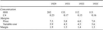
Before discussing our theoretical framework, as a matter of balance, we note two screens which are inconsistent with a story of increased collusion. A high concentration ratio is of course not proof of collusion. Still, insofar as concentration aids the ability of plants to collude, then it is important to note that the macaroni industry was unconcentrated. The top half of Table 2 shows the Herfindahl indicies (HHI) for the industry in each year along with the C4 measure, the total market share of the four largest plants. The HHI starts from a relatively low value in 1929 and falls in 1931 and stays at this low level for the other two censuses. Note that at its peak, the measure is just slightly above 200. The current U.S. Department of Justice Horizontal Merger Guidelines refer to industries with an HHI below 1,000 as “unconcentrated.” On this basis, the macaroni industry would appear to have poor conditions for collusion to take place, at least at the national level.Footnote 8
CONCENTRATION AND MARGIN MEASURES IN THE MACARONI INDUSTRY

Notes:
HHI refers to the Herfendahl index for the macaroni industry with the market defined as the United States. The C4 measure is the market share of the largest four plants. The values for average price, average variable cost, and margin are medians. Values are in cents per pound. These values are for plants which only produce macaroni. Variable cost includes wages, materials, and energy.
Notes:
See the text.
A second screen that does not suggest more collusion is the price-cost margin. In the bottom half of Table 2, we display the median price, variable cost, and margin over time.Footnote 9 Variable cost includes materials, energy, and wages exclusive of salaries. We focus on medians here because there are some outliers that distort the comparison of means. There is no evidence for collusion solely on the basis of price-cost margins, a point noted by Alexander (Reference Alexander1997). In fact, margins are low after considering that these calculations exclude capital costs. Alexander (Reference Alexander1997) does point out that other industries show increasing margins under the NIRA. Increases in margins are the goal of increased collusion. However, Harrington (Reference Harrington and Buccirossi2008) discusses some of the difficulties with using price-cost margins as a measure of collusion. There is empirical evidence that markups are countercyclical, with lower markups during business downturns. Joaquim Martins, Stefano Scarpetta, and Dirk Pilat (Reference Martins, Stefano and Dirk1996) find that 53 of 56 studies showed markups to be countercyclical. However, this need not be driven by changes in competitiveness over the cycle. Various models of sticky prices and wages can generate this pattern. For this reason, we consider price-cost margin one marker among many, while acknowledging higher margins are the goal of collusion.
An alternate source of data for prices in the macaroni industry is a monthly series for wholesale macaroni prices in Chicago calculated by the Bureau of Labor Statistics.Footnote 10 These data are not precisely equivalent to the prices we employ, but reveal a similar pattern of pricing stability under the NIRA. For example, between March 1934 and February 1935, the price was always between 7.6 cents and 8 cents per pound. In March 1935 the price jumped to 9.8 cents, but by July the price was considerably lower, at 7.8 cents, with the bulk of the price change occurring from June to July. For four months at the end of 1935, the wholesale price returned to 9.8 cents. It then fell by 30 percent in one month, and never again returned to its previous level in either real or nominal terms for the remainder of the 1930s. We take this as supportive evidence that the NIRA period was characterized by higher and possibly more stable prices than earlier or later periods. However, other periods, such as May 1932 to February 1933, also saw stable prices, so the evidence is far from conclusive.
AN ORGANIZING FRAMEWORK
Our empirical approach is to examine multiple tests or markers for collusion, as suggested by Harrington (Reference Harrington and Buccirossi2008). He provides a number of tests for collusive behavior, some of which we summarize here. He restricts attention solely to price and market share data because of the limitations on the data that is typically available to economists. Unfortunately, separate data limitations make the implementation of some of his proposed tests problematic for this article, so we supplement these tests with screens using cost data. We stress that none of the tests we employ should separately be thought of as a conclusive evidence for collusion. Instead, taken together, the tests are suggestive evidence of whether or not competition was lessened after the passage of the NIRA.
While the data we use is in some ways more detailed than that which is typically available, in particular the existence of information on cost, it is in other ways more limited. Most notably, there are only four observations per plant, so estimation techniques which rely on high-frequency time series, such as Robert Porter (Reference Porter1983), are infeasible. Also, while information on prices and quantities are observed at the plant level, we have limited information on what markets particular plants were serving, which limits the use of most market power estimation techniques such as Aviv Nevo (Reference Nevo2001). The alternative to our approach would be to build a structural model particular to the macaroni industry. There are many virtues to doing this, such as being able to calculate counterfactuals and quantify welfare losses. The drawback is that many of the inferences drawn will be very sensitive to the model specification.
Although we use several different tests, it is possible to organize our markers within a single modeling framework, that of Athey and Bagwell (Reference Athey and Bagwell2008). Using a repeated Bertrand framework, they examine optimal collusion when plants have persistent cost shocks that are private information. In this setting, there is a tension between productive efficiency, which requires that low-cost plants command most of the market, and incentive constraints, which require that plants not be excessively penalized for revealing themselves as high cost in a given period. This creates a temptation for high-cost plants to mimic the low-cost ones in their pricing decision.Footnote 11 Optimal collusion in this setting leads to price rigidity, where plants' posted prices do not respond to individual cost shocks.Footnote 12
The first test for collusion concerns the relationship between changes in price and changes in marginal cost.
TEST 1: UNDER COLLUSION, THE PRICE RESPONSE OF PLANTS TO COST SHOCKS IS LOWER
The model of Athey and Bagwell (Reference Athey and Bagwell2008) makes a distinction between the pass-through of aggregate versus idiosyncratic cost shocks. The former will be passed through into price completely for the reason because they are known to all cartel members. Therefore, there are no strategic considerations here since the shock affects everyone equally. On the other hand, the pass-through of private cost shocks is less than perfect. These are the shocks that plants must absorb in the rigid price equilibrium to give incentives to plants to truthfully reveal their private information.
This result on price rigidity leads naturally into our other two markers for collusion. Because prices are less sensitive to cost shocks, this implies less variation in prices both within a plant over time and between plants. In fact, they show under certain conditions, such as perfect persistence in cost types, that optimal collusion in the sense of maximizing ex ante profits of a plant entails setting market shares without regard to production costs. When productive efficiency breaks down, then there is a pooling of prices at a single price, which leads to no dispersion in prices in the limit.
Even in the absence of formal theoretical reasoning, competitive markets have been thought to have more dispersed prices than collusive industries. One motivation for the relative stickiness of prices in noncompetitive industries is the risk that price changes could induce a price war (Carlton Reference Carlton, Schmalensee and Willig1989). A number of empirical studies, including Bolotova, Connor, and Miller (Reference Yuliya, Connor and Miller2008), Harrington (Reference Harrington and Buccirossi2008), John Connor (Reference Connor2005), and Abrantes-Metz et al. (Reference Abrantes-Metz, Froeb, Geweke and Taylor2006), have found that after cartels are broken up, price dispersion increases, which provides additional support for our second test.
TEST 2: UNDER COLLUSION, THE DISPERSION OF PRICES IN THE CROSS-SECTION IS LOWER
Consider a simple AR(1) process for detrended prices as a statistical representation of prices.

Then the stationary variance for prices is given by

where 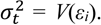 As ρt goes to 1, the process approaches a random walk and the variance grows without bound.
If instead ρt is very close to 0, then the price for a given plant returns very quickly to its long-run average, implying lower levels of dispersion and more stability. Lower persistence follows from a wide class of models of collusive market behavior, not just the model of Athey and Bagwell (Reference Athey and Bagwell2008), as noted in Harrington and Joe Chen (Reference Harrington and Chen2005), but we are unaware of any empirical implementations. Our third test is then is the following.
TEST 3: UNDER COLLUSION, THE PERSISTENCE OF PRICES IS LOWER
Our point in discussing our markers in the context of the Athey and Bagwell (Reference Athey and Bagwell2008) model is not to tie them tightly to particular model. Rather, it is to emphasize the point that these markers are at least a consistent set of tests. There are many models that give rise to each of these predictions which need not be consistent with each other, but our set does not suffer from this deficiency.
The worry with all of these tests is the fact that all of these changes are identified off of only time-series variation. There is no difference-in-difference specification where we take out a common time trend. Furthermore, there are some major aggregate changes occurring, such as the strong recovery in the economy. Julio Rotemberg and Garth Saloner (Reference Julio and Saloner1986) show that with independent and identically distributed (i.i.d.) demand over time, then higher demand increases competitiveness since the returns to deviating on a tacit collusive agreement are highest. Harrington and John Haltiwanger (Reference Harrington and Haltiwanger1991) show that the relationship between aggregate demand and competitiveness relies crucially on the assumption regarding the persistence of demand shocks. We will attempt to address this difficulty by looking at some within industry variation, but, broadly speaking, our empirical results, while consistent with an increase in anti-competitive behavior, do not necessarily pin that on the NIRA versus some other coincident shock.
RESULTS
The implementation of our tests requires defining how we measure costs, in particular marginal costs. For marginal costs, we use the average variable cost, which is the sum of labor costs, material costs, as well as the cost for electricity and fuel, as a proxy for marginal cost. Because of the lack of information about capital costs and salaries, we do not estimate marginal costs directly.Footnote 13 Like the cost variables, the price variable is a unit price calculated as total revenue divided by total output.Footnote 14 The fact that both the independent and dependent variables are derived from a common variable, output, introduces the possibility of nonclassical measurement error. In particular, errors in the output variable will mechanically create a positive correlation between unit prices and costs. We have attempted to address this concern with an instrumental variables strategy based on using percentiles of the contaminated variable.Footnote 15 Results are relatively unaffected.
Aside from the issue of estimating marginal cost, we also face the problem of identifying idiosyncratic shocks to cost. These are the kind of shocks for which the Athey-Bagwell model makes a sharp prediction of low to no pass-through. Aggregate shocks to cost are passed through completely even when plants are colluding in the Athey-Bagwell case. We attempt to control for aggregate shocks to cost through the use of year-fixed effects. The remaining variation in cost is idiosyncratic by construction. The question remains whether the residual changes in cost are known to other competitors.Footnote 16 If these components are known to others, they should also be passed through into price.
To address this issue of whether residual changes in cost are really private information, we also consider the pass-through of labor and materials costs separately. We argue here that changes in labor costs are more likely to be private than those of materials. The reason is that the price of the key materials used in production such as flour is determined in a national market. The cost of labor, on the other hand, is determined at least in part based on local economic conditions. Therefore, a plant in, say, Wisconsin will probably have a good idea of how the cost of flour has changed for a competitor in California but only a guess at how wages have changed. To emphasize, we are not claiming that wages are completely determined locally, only suggesting less variation in materials relative to labor, after removing aggregate shocks. Clearly, there are national wage changes driven by changes in the economy to other legal changes affecting the bargaining power of workers, such as the Wagner Act in 1935.
We also have to address outliers, which are a recurring problem in micro-data. There is large variation in the distribution of average prices, costs, and so on. Some of this is due to measurement error stemming from the self-reported nature of the data. Yet even in modern, well-documented, narrowly defined industries, there is still substantial variation in unit prices, suggesting the same amount of these differences are meaningful (Foster, Haltiwanger, and Syverson Reference Foster, Haltiwanger and Syverson2008). For that reason, we decide to not drop any of the observations, though we explore trimming the 5 percent tails of prices. More precisely, this trimming means we exclude observations where the lagged price is in one of the 5 percent tails.
There is also the question of how to deal with entry and exit. Our basic regressions use changes in the average price as the dependent variable. This necessarily requires that plants be in our data set for two consecutive censuses. This is therefore a special sample of plants that are able to weather an unprecedented decline in the economy. How might this affect the results?
Presumably, the tendency will be for the biggest, most stable plants to survive, and these plants are those most likely to collude along the lines we lay out above. This would possibly lead to a situation where we attribute at least part of the shift in observed behavior to a change in the actual competitive behavior of all plants rather than a composition bias. Whether or not this is actually a problem for us remains to be seen. If the colluding businesses are able to drive out those not part of the conspiracy, we still end up in the same place with anti-competitive behavior. At the same time, it is not difficult to construct stories where the bias would go in the other way and, hence, where the change we observe would be a lower bound in absolute value on the decline in pass-through. Based on this discussion, we have chosen to not attempt to control for the selection, though as we discuss below, if we restrict attention to a common set of plants before and after the NIRA, the main results are unaffected.
There is an issue related to that of selection regarding missing data for certain variables. This is why the sample sizes in some of the tables changes from specification to specification. We choose to include as many observations as possible. We have run the tests restricting attention to a common set of plants with no missing data for any of the key variables, with only minor changes in the results. Also, we treat the observations for 1935 as falling under the NIRA regime, even though the law was invalidated by the Supreme Court in May of that year. If the industry became competitive again in that year, our results understate the magnitude of the effect of the law. Finally, because of the questions about some missing observations in 1929, we experiment with simply dropping all the observations from that year.
TEST 1: PASS-THROUGH
We define a change in (log) price for plant i from period t − 1 to t as δpit , and similarly define the change in (log) costs as δcit. We further define an interaction term δcit ? NIRAt, where NIRAt is a dummy variable for whether or not the change was from 1933 to 1935, when the NIRA code was in effect. The coefficient on the interaction term is the main variable of interest. Specifically, it measures the extent to which the pass-through of cost shocks changes in 1935 relative to the other years. Then the regression we run is
![\[
\begin{array}
\delta p_i,t = \alpha_0 \plus \alpha_1\delta c_i,t \plus \alpha_2[\delta c_i,t * NIRA_t] \plus \rho p_i,t \minus 1 \plus \alphaX_i,t \plus \isin_i,t
\end{array}
\](https://static.cambridge.org/binary/version/id/urn:cambridge.org:id:binary:20160921010034293-0476:S0022050714000618:S0022050714000618_eqnU3.gif?pub-status=live)
where Xi,t are controls including the year- and state-fixed effects. We also include the lagged price pi,t − 1 as an additional regressor. This inclusion makes this specification consistent with the specification we employ later since we will not require prices to follow a random walk, as in Orley Ashenfelter (Reference Foster, Haltiwanger and Syverson1978).
We find evidence consistent with decline in the competitiveness in the macaroni industry based on a fall in pass-through. Table 3 reports regression results of changes in price on changes in cost. In column 1, the pass-through of variable cost shocks is 0.66. That is, a 1 percent increase in average variable costs leads to a 0.66 percent increase in the price charged by the plant and vice versa for a cost decrease. The coefficient on the interaction term is negative and highly significant, evidence for a fall in pass-through in 1935. In other words, prices become stickier in response to cost changes during the period in which the NIRA is in effect, with the pass-through of a 1 percent increase in costs falling to 0.52 percent. In column 2, we run the same regression trimming the 5 percent tails of the lagged price distribution. Column 3 drops state-fixed effect and column 4 drops observations from 1929. The results are broadly similar across all of these alternative specifications with the largest decline in absolute value coming when 1929 observations are excluded.Footnote 17 Another way to express the magnitude of the fall in price responsiveness after the introduction of the NIRA is to consider how the median plant would react to observed cost changes. The median plant's nominal variable costs increase from 4.5 cents per pound in 1933 to 5.6 cents per pound in 1935, an increase of 24 percent. Prior to the NIRA, this would have resulted in an increase in price of 18 percent. After the NIRA, the increase would be 13 percent. These are economically meaningful effects.
PASS-THROUGH OF COST CHANGES INTO PRICE CHANGES

Notes:
* = Significant at the 10 percent level.
** = Significant at the 5 percent level.
*** = Significant at the 1 percent level.
Notes:
Costs are variable costs that include wages, materials, and energy costs. All regressions include year-fixed effects. Standard errors in parenthesis are robust. All variables are in logs.
Source:
See the text.
One potential worry is that increases and decreases in cost may pass-through at different rates. Because we only observe the NIRA during an expansion and earlier periods come from a contraction, this could potentially bias results. In general, prices adjust faster to cost increases than cost decreases (Tappata Reference Tappata2009). However, this phenomenon would actually bias against our result, since input costs rose sharply from 1933 to 1935. This should result in higher pass-through between 1933 and 1935.
The next four columns examine changes in pass-through for labor versus materials costs using the same specification variations as the first four columns. We argued earlier that changes in the rates of pass-through of different types of cost changes provide evidence for collusion along the lines of the Athey-Bagwell model. In particular, we expect greater declines in the pass-through of labor costs relative to materials.Footnote 18 We find differences in baseline pass-through rates that accord with the cost shares of these factors in revenue. Of more interest is that consistently across all four specifications, the pass-through of labor costs falls more than that of materials after the NIRA, sometimes in absolute terms but always in relative terms. The results are not always statistically significant, but the pattern is a consistent one.
TEST 2: DISPERSION
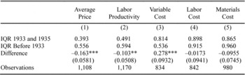
We test for dispersion directly by comparing the interquartile range (IQR) of prices before and after the NIRA with no adjustments made. We use the IQR because it is less sensitive to outliers than the variance. We compare the change in the dispersion of prices to the dispersion in the various cost components. The results are in Table 4, where we include specifications that include and drop observations from 1929. We find very substantial declines in the IQR of prices after the NIRA. The changes are both statistically and economically significant, with a decline of between 33 percent and 20 percent of the pre-NIRA dispersion. Looking at the cost components, there is little change in the dispersion following the NIRA. Columns 3 and 4 of Table 4 show that the IQR for labor productivity decreases by considerably less, falling by 9 percent and 2 percent in each respective specification.
COMPARISON OF INTERQUARTILE RANGES FOR PRICE, LABOR PRODUCTIVITY, VARIABLE COST, WAGES, AND MATERIALS COST

* = Significant at the 10 percent level.
** = Significant at the 5 percent level.
*** = Significant at the 1 percent level.
Notes:
All variables are in logs. Standard errors are calculated using a bootstrap procedure.
Source:
See the text.
COMPARISON OF INTERQUARTILE RANGES FOR PRICE, LABOR PRODUCTIVITY, VARIABLE COST, WAGES, AND MATERIALS COST

* = Significant at the 10 percent level.
** = Significant at the 5 percent level.
*** = Significant at the 1 percent level.
Notes:
The comparisons are of 1929 and 1931 with 1933 and 1935. All variables are in logs. Standard errors are calculated using a bootstrap procedure.
Source:
See the text.
For the variable cost and labor cost variables (columns 5 through 8), we find increases in dispersion, sometimes statistically significant.Footnote 19 Finally, in columns 9 and 10, we find inconsistent changes in the dispersion of materials cost. Taken together, we conclude that the changes in the dispersion of prices is not being driven by changes in the dispersion of the various cost components.
As a robustness check for our definition of the collusive period, we perform the same exercise counting both 1933 and 1935 as under the NIRA. The results using this alternative definition are in Table 5. The IQR of the average price still shows a decline, and the point estimate is close to that observed when classifying only 1935 as under the NIRA. Using the more expansive definition, the decline in the IQR is 0.163, whereas under the narrower definition it is 0.185. After classifying both 1933 and 1935 as NIRA years, there is still a statistically significant increase in the range of variable costs in the later period. Unlike when we use the narrower definition, here we see a decline in the dispersion in labor productivity under the NIRA. Overall, the result of lower dispersion in prices despite unchanged, or even higher, dispersion in costs is robust to the definition of the NIRA period.
VARIANCE COMPARISON FOR RESIDUALS OF PRICE, LABOR PRODUCTIVITY, VARIABLE COST, WAGES, AND MATERIALS COST

Notes:
* = Significant at the 10 percent level.
** = Significant at the 5 percent level.
*** = Significant at the 1 percent level.
Notes:
Residuals are from an AR(1) specification for each of the variables.
Source:
See the text.
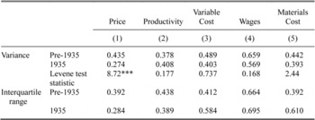
We can also compare the dispersion in the residuals from a reduced form regression for price using a simple AR(1) specification. Using dispersion in the residuals has the advantage that they strip out any changes in the dispersion coming from changes in the persistence of prices, our third test. However, it has the downside that it is model specific and potentially sensitive to specification details. The results reported in Table 6 are consistent with those reported here for the raw prices. Dispersion of price residuals measured by the variance or IQR declines substantially in 1935, with only minor changes for the cost components. Both of these tests provide further evidence consistent with collusion in the NIRA period.
TEST 3: AUTOCORRELATION
Our final test involves examining the autocorrelation in prices. Returning to equation 1, the third test estimates the following modified regression equation
![\[
\begin{array}
\delta p_i,t = \alpha_0 \plus \alpha_1\delta c_i,t \plus \alpha_2[\delta c_i,t * NIRA_t] \plus \rho p_i,t \minus 1 \plus \alphaX_i,t \plus \isin_i,t
\end{array}
\](https://static.cambridge.org/binary/version/id/urn:cambridge.org:id:binary:20160921010034293-0476:S0022050714000618:S0022050714000618_eqnU4.gif?pub-status=live)
This is just a rearrangement of equation 1 where we have added pi, t − 1 to both sides. To be consistent with our previous specification, we include the changes in costs as an additional control.Footnote 20 The coefficient ρ1, the change in the autocorrelation from the pre- to post-NIRA periods, is our coefficient of interest. We run a variant of this regression for variable costs as well as including variable, labor, and material costs. We do so in order to test whether any changes in pricing behavior are being driven by changes in the time-series properties of the input costs at the plant level. This helps rule out explanations for changes observed in the autocorrelation of prices other than changes in the competitive structure.
AUTOCORRELATION FOR PRICE

Notes:
* = Significant at the 10 percent level.
** = Significant at the 5 percent level.
*** = Significant at the 1 percent level.
Notes:
All specifications include year-fixed effects. All variables are in logs. Standard errors are robust.
Source:
See the text.
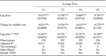
Table 7 presents four different specifications employed in the previous regressions for pass-through. Consistently across all four specifications, we find a substantial decline in the persistence, statistically significant for three out of the four specifications. The magnitude of the NIRA effect is just under one-third of the pre-NIRA persistence in the most conservative specification (column 1) and over two-fifths at the upper end (column 4). The correlation in prices from column 1 at an annual frequency (the square root of the biannual autocorrelation) is 0.82, which is quite close to modern estimates from the CoM in Foster, Haltiwanger, and Syverson (2Reference Foster, Haltiwanger and Syverson008), which are usually around 0.80. This is even after taking into the account the strained comparability between our estimate and the modern one, as modern estimates annualize persistence measures for 5-year intervals versus our biannual frequency. Presumably, plants that survive for five years are relatively stable, and we would expect higher degrees of persistence in prices for this group of relatively stable plants. Unsurprisingly from our previous regressions, changes in cost enter significantly in all of the specifications.
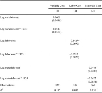
Table 8 shows the change in autocorrelation for the cost components. We find little evidence that the persistence in these variables changed after the introduction of the NIRA. The point estimates on the change are not statistically significant, although they are negative. There is very little evidence of autocorrelation in materials cost either before or during the NIRA, and the autocorrelation in labor costs is small. The evidence suggests that the change in autocorrelation in prices after the introduction of the NIRA was not caused by a change in the autocorrelation of the costs. In other words, the greater stickiness in pricing does not reflect greater stickiness in the determinants of price.
INCORPORATED VERSUS UNINCORPORATED PLANTS
We now consider differences in the effects across a particular cut of the data. In particular, we compare the behavior of incorporated versus unincorporated plants. Harrington (Reference Harrington and Buccirossi2008) notes that an additional way to screen for collusion is to compare the behavior of plants that we have a priori reason to believe are part of the conspiracy, tacit or otherwise, to those who are not. This provides a way to take out changes in behavior that are common across all plants. Our hypothesis is that the incorporated plants were more likely to have been acting collusively. The reason for this is that they were more likely to have had input into the process of drafting the code for the industry. It is less likely that the unincorporated macaroni manufacturers had much influence. Therefore, the code would allocate most of the monopoly profits to the incorporated insiders. Of course, those that draw up the code must make it in the interest for the outsiders to adhere to the code, but they will give the outsiders as little as possible. Therefore, the unincorporated outsiders will be most likely to deviate if conditions change unexpectedly.
AUTOCORRELATION FOR COST COMPONENTS

* = Significant at the 10 percent level.
** = Significant at the 5 percent level.
*** = Significant at the 1 percent level.
Notes:
All specifications include year- and state-fixed effects. All variables are in logs. Standard errors are robust.
Source:
See the text.
Table 9 shows the results for our three tests across these two groups of plants. What we find is that consistently across all three specifications, incorporated plants show a stronger response to the code. The decline in pass-through is larger in absolute and relative terms. The decline in the IQR of prices is more than three times larger for incorporated plants. Finally, the persistence in prices declines by more for incorporated plants after the NIRA comes into effect. These results provide additional support for the view that plants use the code as a coordinating device if, at the same time, some were more willing to follow the rules more closely than others.
TESTS FOR COLLUSION FOR INCORPORATED AND NON-INCORPORATED PLANTS

* = Significant at the 10 percent level.
** = Significant at the 5 percent level.
*** = Significant at the 1 percent level.
Notes:
First two columns repeat first test for collusion comparing pass-through. Second two columns compare interquartile range of prices. Last two columns examine the persistence in prices. Regressions for first and third test include state- and year-fixed effects. All variables are in logs. Standard errors in parenthesis are robust for first and third set of results. Standard errors for second set of results are calculated using a bootstrap procedure.
Source:
See the text.
CONCLUSION
This article has revisited the question of collusion under the NIRA with both new data and a new methodology using plant-level data from the Census of Manufactures for the macaroni industry. Others have argued that the macaroni industry provides an example for why collusion failed in a wide swath of industries: heterogeneity in costs. Our results contradict this view. While we see no major change in HHI, C4, or price-cost margins after the NIRA is instituted, using a variety of markets for collusion, we find evidence that collusion was indeed taking place. First, there was a significant decrease in cost pass-through after the NIRA was introduced. Second, the dispersion of prices fell in the cross-section after the NIRA. Finally, the persistence in prices also declined.
From a broader perspective, recent work in macroeconomics by Harold L. Cole and Lee Ohanian (Reference Cole and Lee2004) and by Eggertsson (Reference Eggertsson2012) has focused on how the NIRA shifts the aggregate supply relationship leftward. While these papers differ in how they evaluate the effects of these policies overall, they both agree that the effect of the NIRA was a negative supply shock. Cole and Ohanian (Reference Cole and Lee2004) take a neoclassical view and end up with a result that decreases in competitiveness lead to declines in output. Eggertsson (Reference Eggertsson2012) argues that when the economy is in a liquidity trap, anything that pushes up inflation expectations speeds recovery, and cartelizing a vast part of the economy could do so. In that model, the aggregate demand curve actually slopes upward, and increases in inflation expectations lead to reductions in real interest rates. With a reduction in the real interest rates comes an increase in investment and output. Both share a common belief in how the NIRA shifted the aggregate supply relationship. However, both have little to say about the fact that the recovery is not complete until 1941.
Our results lead us to reconsider the discussion in Christina Romer (Reference Romer1999). In that paper, she discusses why prices continued to rise in the 1930s after the nadir of the Depression. Though this was a time of rapid growth, the deviation in output from potential output was still quite large. Any model of price adjustment would have implied deflation rather than continued inflation during this period, given the massive slack in the economy. While arguing that part of the inflation can be explained by the rapid growth after 1933, Romer argues that the NIRA slowed the usual adjustment process of short-run aggregate supply to a decline in aggregate demand. The NIRA slowed adjustment by encouraging prices based on “average unit costs in a year of normal output rather than based on actual (but not easily observed) overhead costs” (pg. 189). We think of our results as providing some micro-evidence for Romer's own conclusion: “Thus, the [NIRA] can best be thought of as a force holding back recovery, rather than as one actively depressing output.” In other words, it lead to a slower recovery, not a deeper recession.
In the end, virtually any pricing behavior can be rationalized as noncompetitive. As quoted by William Landes, Ronald Coase once remarked that he had become “tired of antitrust because when the prices went up the judges said it was monopoly, when the prices went down they said it was predatory pricing, and when they stayed the same they said it was tacit collusion” (Kitch Reference Kitch1983). This is an important caveat to always turning to a noncompetitive explanation. Individually, it would be easy to dismiss these results as providing limited evidence for collusion. However, taken together as a whole, we argue that they are best explained by an increase in collusive behavior driven by the NIRA. We started with an industry that was previously argued to have been unaffected by the NIRA. This suggests that an increase in anti-competitive behavior was common to a broader set of industries. However, this suggestion is no substitute for actual data on how these other industries behaved.
Data Appendix: Calculating Costs for Multiproduct Plants
Whereas in the output case where we have a breakdown of revenue by product group, plants only reported their total costs not their costs product type by product type. So to construct an average cost we have to parcel the total cost into costs of production for each type of good. We have experimented with different approaches here. What we use in the article to calculate an average cost is the following. Assume that the cost of producing good j for plant i is given by cji = cj + εi . This structure allows for plants to differ in their productivity levels εi and for products to differ in their costs cj . We do not allow any correlation between these two components. Let c_ i denote plant i's total cost, then we can solve for εi as

where qji is the production of good j by plant i. We assume that we can estimate cj by restricting attention to plants that only produce that product. Once we have calculated εi , the average cost for multiproduct plant i is the real output weighted average of the costs to produce each product plus our plant productivity estimate εi . Note that we take a similar approach to calculating the average price.
We have also ran regressions restricting attention to plants that only produce macaroni. This is actually the vast majority of plants and results appear nearly unchanged. Another approach is to assume that the cost of producing the various goods is the same at the plant level. This means that we simply sum up total physical output of each product and divide total costs by this amount to get an average. This too gives similar results.