


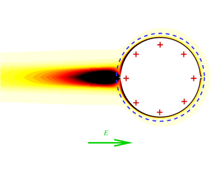


1 Introduction
Electrophoresis refers to the motion of charged colloidal particles or macromolecules in a liquid electrolyte subjected to an external electric field (Saville Reference Saville1977; Russel, Saville & Schowalter Reference Russel, Saville and Schowalter1989). When the particle is immersed in the electrolyte, an electrical double layer develops around the particle surface, consisting of an immobile layer of surface charge and a diffuse cloud, called the Debye layer, that is enriched in counter-ions. Under the applied field, the particle motion is determined by the balance of three forces, i.e. the electric force, the viscous drag and the retardation force, the last of which accounts for the extra drag due to the ion cloud moving in the direction opposite to the particle motion. Electrophoresis plays an important role in colloid science (Russel et al. Reference Russel, Saville and Schowalter1989), bio-analysis (Kostal, Katzenmeyer & Arriaga Reference Kostal, Katzenmeyer and Arriaga2008) and many other applications in microfluidic devices (Chang & Yeo Reference Chang and Yeo2010). For example, gel electrophoresis or capillary electrophoresis, which separates molecules such as DNA, RNA or proteins based on their size and charge in polymer solutions, has been developed into an indispensable technique in biochemistry (Southern Reference Southern1975; Barron, Soane & Blanch Reference Barron, Soane and Blanch1993). Electrophoretic deposition techniques with non-aqueous solvents and polymer binders have been widely used in manufacturing of complex-shaped ceramics and glasses, solid oxide fuel cells and hybrid materials (Besra & Liu Reference Besra and Liu2007). Despite these important applications, there have been few studies on the effects of polymer viscoelasticity on electrophoresis. Some previous studies have discussed DNA electrophoresis using scaling theories for entangled polymer molecules (Barron et al. Reference Barron, Soane and Blanch1993; Duke & Viovy Reference Duke and Viovy1994), but the detailed electrohydrodynamics of electrophoresis in a polymer solution has not yet been considered.
One of the key questions about electrophoresis is the dependence of particle velocity on the physical properties involved in the problem, such as the strength of the applied field, fluid viscosity, zeta potential and particle size. There has been a long history of calculating the electrophoretic velocity of a particle using theories with increasing complexity and numbers of factors in consideration. In the limit of zero double-layer thickness, Smoluchowski (Reference Smoluchowski1903) derived the dimensional (represented by the superscript  $^{\ast }$) speed of a spherical particle as
 $$\begin{eqnarray}U^{\ast }=\frac{\unicode[STIX]{x1D700}\unicode[STIX]{x1D700}_{0}E^{\ast }\unicode[STIX]{x1D701}^{\ast }}{\unicode[STIX]{x1D707}},\end{eqnarray}$$
where  $E^{\ast }$ is the strength of the electric field,
 $\unicode[STIX]{x1D701}^{\ast }$ is the zeta potential, and
 $\unicode[STIX]{x1D700},~\unicode[STIX]{x1D700}_{0}$ and
 $\unicode[STIX]{x1D707}$ are the dielectric constant, the vacuum permittivity and the viscosity of the electrolyte. Equation (1.1), which holds for a particle of uniform zeta potential, was later proved to be universally valid for particles of any size, shape and orientation relative to the applied field, as long as the double-layer thickness is much smaller than the particle size (Morrison Reference Morrison1970). Sellier (Reference Sellier1999) showed it applies to a collection of particles of arbitrary size, shape and equal zeta potential.
Under the Debye–Hückel assumption ( $\unicode[STIX]{x1D701}^{\ast }e/kT\ll 1$, where
 $kT/e$ is the thermal voltage), Henry (Reference Henry1931) studied the electrophoresis of a sphere with an arbitrary double-layer thickness. If the double layer is much thicker than the particle size, the velocity is two-thirds that given by (1.1). Both Smoluchowski’s and Henry’s solutions assumed the diffusive ion cloud around the particle is in equilibrium and follows a Boltzmann distribution. For a moderately charged particle (
 $\unicode[STIX]{x1D701}^{\ast }e/kT\sim O(1)$), for which the Debye–Hückel approximation is no longer valid while surface conduction is still negligible, the large counter-ion concentration near the particle surface generates a strong non-uniform tangential current inside the double layer, which leads to a normal ion flux that deforms the double layer and eventually affects the particle velocity. The analysis considering this effect was performed in a weak applied field by O’Brien & Hunter (Reference O’Brien and Hunter1981) and was extended to particles of arbitrary shape (O’Brien Reference O’Brien1983) and of high zeta potential (Schnitzer & Yariv Reference Schnitzer and Yariv2012a). The particle velocity shows a non-monotonic variation with the zeta potential, consistent with numerical simulations (Wiersema, Loeb & Overbeek Reference Wiersema, Loeb and Overbeek1966; O’Brien & White Reference O’Brien and White1978).
In recent years, the topic has been extended to consider the effects of boundaries (Yariv Reference Yariv2006), nonlinear particle velocity due to the higher-order terms in the weak field expansion (Schnitzer et al. Reference Schnitzer, Zeyde, Yavneh and Yariv2013), strong fields (Schnitzer & Yariv Reference Schnitzer and Yariv2012b), oscillating electric fields (Mangelsdorf & White Reference Mangelsdorf and White1992; Sawatzky & Babchin Reference Sawatzky and Babchin1993) and soft particles (Ohshima Reference Ohshima2013). More numerical simulations of electrophoresis of a single particle can be found in a recent review by Zhou & Schmid (Reference Zhou and Schmid2015). The electrophoresis of a single particle is important because it serves as a basis for many electrokinetic phenomena, such as electroacoustics and electrorheology (Saville Reference Saville1977).
In many electrokinetic applications, the fluids are non-Newtonian. In electrophoretic separations, uncrosslinked polymer solutions (Barron et al. Reference Barron, Soane and Blanch1993) or crosslinked gel matrices (Woolley & Mathies Reference Woolley and Mathies1994) are used to introduce a molecular-weight dependence to DNA’s electrophoretic mobility. Electro-osmotic flow of non-Newtonian fluids is also found in some microfluidic devices (Chang & Yeo Reference Chang and Yeo2010) and in polymer electrolytes for batteries (Wei et al. Reference Wei, Cheng, Nath, Tikekar, Li and Archer2018). Electro-osmotic flows with shear-rate-dependent viscosity and viscoelasticity have both been analysed in previous studies, and references can be found in a recent review by Zhao & Yang (Reference Zhao and Yang2013). It is worth noting that, since polymer elasticity does not affect the unidirectional flow, the major effect of a non-Newtonian fluid in these flows is due to the shear-thinning viscosity (Afonso, Alves & Pinho Reference Afonso, Alves and Pinho2009; Zhao & Yang Reference Zhao and Yang2009).
For electrophoresis in a polymeric electrolyte, previous studies used the Debye–Büche–Brinkman model to study the effects of the porous structure of a polymer gel on the particle velocity (Debye & Bueche Reference Debye and Bueche1948). Other studies have considered non-Newtonian suspending fluids and emphasized the effects of shear-dependent viscosity. Based on Newton’s second law for a particle moving in a fluid with a nonlinear friction coefficient, Vidybida & Serikov (Reference Vidybida and Serikov1985) suggested that net motion of a spherical particle under an oscillating electric field is possible in non-Newtonian fluids. Numerical simulations by Hsu, Hung & Yu (Reference Hsu, Hung and Yu2004), Lee, Chen & Hsu (Reference Lee, Chen and Hsu2005) and Hsu, Yeh & Ku (Reference Hsu, Yeh and Ku2006) show that the mobility of a particle increases in a shear-thinning Carreau fluid, and this effect is more pronounced for a thinner double layer (Hsu et al. Reference Hsu, Yeh and Ku2006). Khair, Posluszny & Walker (Reference Khair, Posluszny and Walker2012) analytically studied the electrophoresis of a particle with a thin double layer in a Carreau fluid. Their analysis shows that shear-thinning/thickening viscosity increases/decreases the particle velocity with effects arising from flows both inside and outside the double layer. The non-Newtonian rheology leads to a size-dependent particle velocity, in contrast to the results for a Newtonian fluid. As we will see later, at low  $Wi=\unicode[STIX]{x1D706}U^{\ast }/a$, where
 $\unicode[STIX]{x1D706}$ is the polymer relaxation time and
 $a$ is the particle radius, the shear-thinning viscosity of a polymer solution has the same effects on the electrophoretic particle. Its contribution mainly comes from the double layer because of the high local shear rate. However, at high
 $Wi$, the polymers are strongly deformed and the particle velocity is mainly affected by polymer elasticity.
The electrokinetic flow around a spherical particle is strongly influenced by viscoelasticity due to two factors. First, there are large changes of shear rate as a polymer enters and leaves the high-shear region of the double layer so that the time history of the flow in a Lagrangian frame will have a large effect. Second, polymers are strongly deformed near the stagnation points at the front and back of the sphere, modifying the flow field in these regions. The rear stagnation point leads to a region of high polymer stress known as a ‘birefringent strand’, which has been widely studied in the motion of a particle/bubble in a polymer solution driven by a body force (Harlen Reference Harlen1990; Harlen, Rallison & Chilcott Reference Harlen, Rallison and Chilcott1990; Arigo et al. Reference Arigo, Rajagopalan, Shapley and McKinley1995; Fabris, Muller & Liepmann Reference Fabris, Muller and Liepmann1999). It causes a large local extensional viscosity (Harlen et al. Reference Harlen, Rallison and Chilcott1990), increases the drag on the particle and leads to an extended wake behind the particle (Arigo et al. Reference Arigo, Rajagopalan, Shapley and McKinley1995; Fabris et al. Reference Fabris, Muller and Liepmann1999). Harlen (Reference Harlen1990) and Harlen et al. (Reference Harlen, Rallison and Chilcott1990) studied the birefringent strand downstream of a stagnation point by treating it as a distribution of stokeslets to calculate the extra stress exerted by the polymer. With a fitting parameter, which characterizes the strength of the polymer stress, their results accurately reproduced the downstream velocity profile and the drag coefficient measured in experiments and simulations. Two types of stagnation points were discussed in their work. Near an isolated stagnation point, such as on the slip surface of a bubble, the strain rate is approximately constant and the birefringent strand starts from the stagnation point. On a no-slip surface, the polymer is undeformed at the stagnation point and the strand starts at a point downstream where the local strain rate exceeds the critical value. Becherer, van Saarloos & Morozov (Reference Becherer, van Saarloos and Morozov2008, Reference Becherer, van Saarloos and Morozov2009) also studied the scaling of the width and extension of the strand as well as its singularity in two-dimensional purely elongational flows.
In this work, we will see that the birefringent strand behind an electrophoretic particle has many similarities to the previous studies. The polymer flow near the rear stagnation point outside and inside the double layer resembles the extensional flow around a bubble and solid sphere, respectively. The unique aspect of viscoelastic electrokinetic flows around a sphere is that polymers can also be strongly stretched by a shear flow inside the double layer. Compared to an extensional stretch, for which polymer deformation increases abruptly when the local strain rate is above a critical value, polymer stretch in a shear flow grows more smoothly with increasing shear rate. If the double-layer thickness is small enough, full polymer extension in the shear flow could occur earlier than that due to the extensional flow.
The interaction of particles with viscoelastic fluids has been considered in many previous studies, including the gravity-driven motion of a sphere in a viscoelastic fluid (Leslie & Tanner Reference Leslie and Tanner1961; Chilcott & Rallison Reference Chilcott and Rallison1988; Harlen Reference Harlen1990; Harlen et al. Reference Harlen, Rallison and Chilcott1990), migration of a particle in wall-bounded shear flow of a second-order fluid (Ho & Leal Reference Ho and Leal1976), the motion of a sphere normal to a wall (Ardekani, Rangel & Joseph Reference Ardekani, Rangel and Joseph2007), the interactions of two spheres (Ardekani, Rangel & Joseph Reference Ardekani, Rangel and Joseph2008; Khair & Squires Reference Khair and Squires2010) and the rheology of a dilute particle suspension in a polymeric fluid (Koch & Subramanian Reference Koch and Subramanian2006; Rallison Reference Rallison2012; Koch, Lee & Mustafa Reference Koch, Lee and Mustafa2016; Yang & Shaqfeh Reference Yang and Shaqfeh2018; Einarsson, Yang & Shaqfeh Reference Einarsson, Yang and Shaqfeh2018), etc. In many studies, the generalized reciprocal theorem (Cox Reference Cox1965; Ho & Leal Reference Ho and Leal1974) has been applied to calculate the drag or stresslet without the need to derive the fluid velocity at higher orders. Based on a perturbation in  $Wi$, Chilcott & Rallison (Reference Chilcott and Rallison1988) derived the formula for the drag on a sphere of arbitrary viscosity ratio to the fluid. To explore the behaviour of polymers at finite
 $Wi$, Koch et al. (Reference Koch, Lee and Mustafa2016) conducted a perturbation in the polymer concentration and calculated the particle stresslet by a numerical integration along the undisturbed streamlines. Weak coupling between polymer deformation and the fluid velocity for a dilute polymer solution was also applied in simulations (Wapperom & Renardy Reference Wapperom and Renardy2005; Moore & Shelley Reference Moore and Shelley2012). Such techniques will be employed in this study for both asymptotically small and finite
 $Wi$.
In recent years, the interaction of self-propelled particles with polymeric fluids has attained great interest in order to understand the motion of micro-organisms and self-propelled colloids in complex fluids (Zhu, Lauga & Brandt Reference Zhu, Lauga and Brandt2012; Li, Karimi & Ardekani Reference Li, Karimi and Ardekani2014; Datt et al. Reference Datt, Natale, Hatzikiriakos and Elfring2017; Natale et al. Reference Natale, Datt, Hatzikiriakos and Elfring2017). These studies typically neglect the detailed swimming mechanisms of the particles, for example, the metachronal waves on the ciliated surface of Volvox and the self-generated gradients of chemical species or temperature that drive diffusiophoresis or thermophoresis (Howse et al. Reference Howse, Jones, Ryan, Gough, Vafabakhsh and Golestanian2007). Instead, they use the squirmer model (Lighthill Reference Lighthill1952; Blake Reference Blake1971) with a prescribed slip velocity on the surface of the particle that is not affected by the polymer. Squirmer motions in a fluid with weak viscoelasticity (Datt & Elfring Reference Datt and Elfring2019) or non-uniform viscosity (Shoele & Eastham Reference Shoele and Eastham2018) have been studied using the generalized reciprocal theorem. However, in view of the high shear rates in the region where the slip is generated, polymers should affect the effective slip velocity seen by the outer flow field. Similar to other types of phoretic particles, an electrophoretic particle creates an outer flow consistent with the squirmer model and the slip velocity can be understood in terms of the flow generated in the thin double layer. In particular, an electrophoretic particle with a uniform zeta potential in a Newtonian fluid is a neutral-type squirmer, i.e. the far field of the particle motion does not have a contribution due to a stokeslet dipole. As we will see later, the polymer deformation inside the double layer is very important. In a weakly viscoelastic fluid, the leading-order effect of the polymer comes solely from the inner region and the polymer elasticity changes the particle into a puller-type squirmer. At high  $Wi$, the strong polymer stretching inside the double layer significantly affects the particle velocity. While the polymeric effects in the bulk region always reduce the particle velocity, those arising inside the double layer can either increase or decrease the velocity depending on
 $Wi$.
In this work, we present a theoretical framework to calculate the electrophoretic velocity of a spherical particle in a viscoelastic fluid, based on a perturbation in the polymer concentration  $c$. In § 2, we describe the governing equations of the problem. Next, § 3 discusses the
 $O(c)$ modification of the slip velocity due to polymers inside the double layer and the procedure to find the fluid and particle velocities. In § 4, we discuss a different method, i.e. using the generalized reciprocal theorem, to find the particle’s electrophoretic velocity and avoid solving the polymer-induced perturbation to the fluid velocity. To understand how the polymer affects electrophoresis, we then discuss the polymer deformation outside and inside the double layer in §§ 5 and 6, respectively. We analyse the evolution of polymer deformation along the symmetry axis of the particle as well as on its slip and no-slip surfaces and estimate the length and radius of the birefringent strand. These results are later used to predict the scaling of the particle velocity. In § 7, we consider the problem for
 $Wi\ll 1$ and use the two methods in §§ 3 and 4 to derive the
 $O(Wi)$ fluid velocity and the
 $O(Wi^{2})$ non-trivial particle velocity. Finally, § 8 shows the particle velocity at high
 $Wi$ through a numerical realization of the generalized reciprocal theorem.
2 Governing equations
We consider a spherical solid particle of radius  $a$ in a binary electrolyte solution with valences
 $\pm z$, dielectric constant
 $\unicode[STIX]{x1D700}$ and solvent viscosity
 $\unicode[STIX]{x1D707}$. The particle is insulating with a uniform zeta potential, so no calculation for the particle interior is needed. The polymer concentration
 $c=\unicode[STIX]{x1D707}^{p}/\unicode[STIX]{x1D707}\ll 1$, where
 $\unicode[STIX]{x1D707}^{p}$ and
 $\unicode[STIX]{x1D707}$ are the polymer and solvent contributions to the zero-shear-rate viscosity, respectively. In what follows, lengths are normalized by
 $a$, velocities by the electrophoretic velocity
 $U^{\ast }=\unicode[STIX]{x1D700}\unicode[STIX]{x1D700}_{0}E^{\ast }\unicode[STIX]{x1D701}^{\ast }/\unicode[STIX]{x1D707}$ in a Newtonian fluid, times by
 $a/U^{\ast }$, stresses by
 $\unicode[STIX]{x1D707}U^{\ast }/a$, potentials by
 $\unicode[STIX]{x1D713}_{0}=kT/ze$, electric fields by
 $\unicode[STIX]{x1D713}_{0}/a$, and ion concentrations by the far-field concentration
 $n_{\infty }$. Here,
 $\unicode[STIX]{x1D700}_{0}$ is the vacuum permittivity,
 $kT$ is the Boltzmann temperature, and
 $e$ is the elementary charge. The governing equations for the steady incompressible Stokes flow, the electric field and the ion concentration are, respectively, the Stokes, Poisson and Nernst–Planck equations:
 $$\begin{eqnarray}\displaystyle & \displaystyle E\unicode[STIX]{x1D701}(\unicode[STIX]{x1D735}\boldsymbol{\cdot }\unicode[STIX]{x1D748}+\unicode[STIX]{x1D735}\boldsymbol{\cdot }\unicode[STIX]{x1D749})+\unicode[STIX]{x1D6FB}^{2}\unicode[STIX]{x1D713}\unicode[STIX]{x1D735}\unicode[STIX]{x1D713}=0,\quad \unicode[STIX]{x1D735}\boldsymbol{\cdot }\boldsymbol{u}=0, & \displaystyle\end{eqnarray}$$
 $$\begin{eqnarray}\displaystyle & \displaystyle 2\unicode[STIX]{x1D6FB}^{2}\unicode[STIX]{x1D713}=-\unicode[STIX]{x1D705}^{2}(n^{+}-n^{-}), & \displaystyle\end{eqnarray}$$
 $$\begin{eqnarray}\displaystyle & \displaystyle E\unicode[STIX]{x1D701}Pe(\boldsymbol{u}-\boldsymbol{U})\boldsymbol{\cdot }\unicode[STIX]{x1D735}n^{\pm }=\unicode[STIX]{x1D735}\boldsymbol{\cdot }(\unicode[STIX]{x1D735}n^{\pm }\pm n^{\pm }\unicode[STIX]{x1D735}\unicode[STIX]{x1D713}). & \displaystyle\end{eqnarray}$$
We adopt a reference frame with a moving particle and the fluid at rest at infinite separation from the particle throughout the paper. In this reference frame,  $n^{\pm }$ are unsteady. However, for a steady electrophoretic velocity,
 $n^{\pm }$ are stationary in a reference frame moving with the particle, and this observation allows us to replace the time derivative in (2.1c) by a convective term associated with the motion of the centre of mass of the particle. Here
 $E=E^{\ast }a/\unicode[STIX]{x1D713}_{0}$,
 $\unicode[STIX]{x1D701}=\unicode[STIX]{x1D701}^{\ast }/\unicode[STIX]{x1D713}_{0}$,
 $\unicode[STIX]{x1D748}=-p\unicode[STIX]{x1D644}+2\unicode[STIX]{x1D64E}$ is the Newtonian stress,
 $p$ is pressure,
 $\unicode[STIX]{x1D644}$ is the identity matrix,
 $\unicode[STIX]{x1D64E}=(\unicode[STIX]{x1D735}\boldsymbol{u}^{\text{T}}+\unicode[STIX]{x1D735}\boldsymbol{u})/2$ is the strain-rate tensor,
 $\boldsymbol{u}$ is fluid velocity,
 $\boldsymbol{U}$ is particle velocity,
 $\unicode[STIX]{x1D749}$ is polymer stress,
 $\unicode[STIX]{x1D713}$ is electric potential,
 $n^{\pm }$ are the concentrations of positive and negative ions, and
 $\unicode[STIX]{x1D705}$ is the inverse of the double-layer thickness, with
 $\unicode[STIX]{x1D705}^{2}=2z^{2}e^{2}n_{\infty }a^{2}/(\unicode[STIX]{x1D700}\unicode[STIX]{x1D700}_{0}kT)$. The Péclet number
 $Pe=U_{0}a/D$ is independent of particle dimensions and electrolyte concentration, where
 $U_{0}=\unicode[STIX]{x1D700}\unicode[STIX]{x1D700}_{0}(kT)^{2}/(z^{2}e^{2}\unicode[STIX]{x1D707}a)$ is a thermal velocity derived by balancing the characteristic Maxwell stress
 $\unicode[STIX]{x1D700}\unicode[STIX]{x1D700}_{0}(\unicode[STIX]{x1D713}_{0}/a)^{2}$ and the viscous stress
 $\unicode[STIX]{x1D707}U_{0}/a$. For simplicity, we consider equal cation and anion diffusivities,
 $D=D^{+}=D^{-}$. In typical aqueous solutions
 $Pe=0.5$ (Saville Reference Saville1977), although it can be smaller in a viscous electrolytic solution where the ions do not satisfy the Stokes–Einstein relationship (Wei et al. Reference Wei, Cheng, Nath, Tikekar, Li and Archer2018). In this study,
 $Pe$ does not affect the electrophoresis because the ion distribution is uniform in the bulk region and the convection in the double layer is negligible at small zeta potential.
For the polymer stresses, we consider several different continuum models to investigate the effects of finite extensibility and shear thinning. The continuum model is valid for an electrolyte with a small salt concentration ( ${\sim}1~\text{mM}$) and polymers of relatively small molecular weight (
 ${\sim}10^{4}$), where the radius of gyration of the polymer (
 ${\sim}1~\text{nm}$) is smaller than the double-layer thickness (
 ${\sim}10~\text{nm}$). For a polymer solution, the general form for the polymer stress can be written as
 $$\begin{eqnarray}\unicode[STIX]{x1D749}=\frac{c}{Wi}\boldsymbol{F}(\unicode[STIX]{x1D63C}),\end{eqnarray}$$
where the Weissenberg number  $Wi=\unicode[STIX]{x1D706}U^{\ast }/a$ is defined as the polymer relaxation time times the characteristic shear rate
 $U^{\ast }/a$. Here
 $\unicode[STIX]{x1D63C}$ is the polymer conformation tensor governed by the constitutive equation
 $$\begin{eqnarray}\overset{\,\,\triangledown }{\unicode[STIX]{x1D63C}}=\frac{1}{Wi}\boldsymbol{G}(\unicode[STIX]{x1D63C}),\end{eqnarray}$$
where  $\overset{\,\,\triangledown }{\unicode[STIX]{x1D63C}}$ denotes the upper-convected derivative,
 $$\begin{eqnarray}\overset{\,\,\triangledown }{\unicode[STIX]{x1D63C}}=\frac{\unicode[STIX]{x2202}\unicode[STIX]{x1D63C}}{\unicode[STIX]{x2202}t}+\boldsymbol{u}\boldsymbol{\cdot }\unicode[STIX]{x1D735}\unicode[STIX]{x1D63C}-\unicode[STIX]{x1D735}\boldsymbol{u}^{\text{T}}\boldsymbol{\cdot }\unicode[STIX]{x1D63C}-\unicode[STIX]{x1D63C}\boldsymbol{\cdot }\unicode[STIX]{x1D735}\boldsymbol{u}.\end{eqnarray}$$
For different models,  $\boldsymbol{F}(\unicode[STIX]{x1D63C})$ and
 $\boldsymbol{G}(\unicode[STIX]{x1D63C})$ are (Bird & Wiest Reference Bird and Wiest1995)
 $$\begin{eqnarray}\left.\begin{array}{@{}rl@{}}\text{Oldroyd-B:} & \quad \boldsymbol{F}(\unicode[STIX]{x1D63C})=\unicode[STIX]{x1D63C}-\unicode[STIX]{x1D644},\quad \boldsymbol{G}(\unicode[STIX]{x1D63C})=\unicode[STIX]{x1D644}-\unicode[STIX]{x1D63C},\\ \text{Giesekus:} & \quad \boldsymbol{F}(\unicode[STIX]{x1D63C})=\unicode[STIX]{x1D63C}-\unicode[STIX]{x1D644},\quad \boldsymbol{G}(\unicode[STIX]{x1D63C})=\unicode[STIX]{x1D644}-\unicode[STIX]{x1D63C}-\unicode[STIX]{x1D6FC}(\unicode[STIX]{x1D63C}-\unicode[STIX]{x1D644})^{2},\\ \text{FENE-P:} & \quad \boldsymbol{F}(\unicode[STIX]{x1D63C})=f\unicode[STIX]{x1D63C}-b\unicode[STIX]{x1D644},\quad \boldsymbol{G}(\unicode[STIX]{x1D63C})=b\unicode[STIX]{x1D644}-f\unicode[STIX]{x1D63C},\\ \text{FENE-CR:} & \quad \boldsymbol{F}(\unicode[STIX]{x1D63C})=f\unicode[STIX]{x1D63C}-f\unicode[STIX]{x1D644},\quad \boldsymbol{G}(\unicode[STIX]{x1D63C})=f\unicode[STIX]{x1D644}-f\unicode[STIX]{x1D63C}.\end{array}\right\}\end{eqnarray}$$
The Oldroyd-B model has a shear viscosity and normal stress coefficients that are independent of shear rate, which allows one to study the effects of fluid viscoelasticity in the absence of shear thinning. It describes well Boger fluids, which are dilute solutions of high-molecular-weight polymers in viscous Newtonian fluids. However, above a critical Weissenberg number, the Oldroyd-B model predicts an infinite extensional viscosity and becomes unphysical in an extensional flow. This issue is resolved in the three other models. The Giesekus model has an anisotropic relaxation rate of the polymers as well as a shear-thinning viscosity. In it,  $\unicode[STIX]{x1D6FC}$ is the mobility factor representing the anisotropic hydrodynamic drag on the polymer molecule and must lie between 0 and
 $1/2$ to ensure a linearly stable solution and positive definite conformation tensor for a steady shear flow (Schleiniger & Weinacht Reference Schleiniger and Weinacht1991). For the FENE (finitely extensible nonlinear elastic) models, the polymer is restricted by a finite extensibility. In them,
 $L$ is the maximum length of the polymer,
 $f=L^{2}/(L^{2}-\text{tr}(\unicode[STIX]{x1D63C}))$, and
 $b=L^{2}/(L^{2}-3)$. The FENE-P model has a shear-thinning viscosity, while the FENE-CR model has a constant viscosity. The Giesekus model is often used for entangled polymer solutions and worm-like micelles (Helgeson et al. Reference Helgeson, Reichert, Hu and Wagner2009), whereas FENE models are for dilute solutions. For
 $\unicode[STIX]{x1D6FC}=0$ and
 $L\rightarrow \infty$, all the models recover the Oldroyd-B model.
The boundary conditions at the particle surface include no slip, Gauss law and zero ion fluxes, i.e.
 $$\begin{eqnarray}\text{at }r=1:\quad u_{r}=U\cos \unicode[STIX]{x1D703},\quad u_{\unicode[STIX]{x1D703}}=-U\sin \unicode[STIX]{x1D703},\quad -\frac{\unicode[STIX]{x2202}\unicode[STIX]{x1D713}}{\unicode[STIX]{x2202}r}=q,\quad \frac{\unicode[STIX]{x2202}n^{\pm }}{\unicode[STIX]{x2202}r}\pm n^{\pm }\frac{\unicode[STIX]{x2202}\unicode[STIX]{x1D713}}{\unicode[STIX]{x2202}r}=0,\end{eqnarray}$$
where  $q=zeQ/(4\unicode[STIX]{x03C0}a\unicode[STIX]{x1D700}\unicode[STIX]{x1D700}_{0}kT)$ is the normalized surface charge density for a particle of total charge
 $Q$,
 $U$ is the dimensionless particle speed, and
 $\unicode[STIX]{x1D703}$ is the polar angle measured from the direction of the particle velocity. In the Debye–Hückel limit,
 $q=\unicode[STIX]{x1D701}\unicode[STIX]{x1D705}$, with
 $\unicode[STIX]{x1D701}$ being the potential on the particle surface (Russel et al. Reference Russel, Saville and Schowalter1989). Far away from the particle, the boundary conditions are
 $$\begin{eqnarray}\text{as }r\rightarrow \infty :\quad u_{r}=0,\quad u_{\unicode[STIX]{x1D703}}=0,\quad \unicode[STIX]{x1D713}=-Er\cos \unicode[STIX]{x1D703},\quad n^{\pm }=1,\quad \unicode[STIX]{x1D63C}=\unicode[STIX]{x1D644},\end{eqnarray}$$
where the ion concentration, fluid and polymer are undisturbed, and the potential recovers the applied field. The force balance on the particle provides the condition for calculating the particle velocity  $U$, i.e. the sum of Newtonian, polymer and Maxwell stresses on the particle surface vanishes,
 $$\begin{eqnarray}\int _{r=1}\left[E\unicode[STIX]{x1D701}(\unicode[STIX]{x1D748}+\unicode[STIX]{x1D749})+\unicode[STIX]{x1D735}\unicode[STIX]{x1D713}\unicode[STIX]{x1D735}\unicode[STIX]{x1D713}-{\textstyle \frac{1}{2}}\unicode[STIX]{x1D735}\unicode[STIX]{x1D713}\boldsymbol{\cdot }\unicode[STIX]{x1D735}\unicode[STIX]{x1D713}\unicode[STIX]{x1D644}\right]\boldsymbol{\cdot }\boldsymbol{n}\,\text{d}A=0,\end{eqnarray}$$
where  $\boldsymbol{n}$ is the outward unit normal vector on the particle surface.
3 Regular perturbation in polymer concentration
We seek a regular perturbation solution for low polymer concentration  $c\ll 1$. Since the polymer deformation does not directly affect the ion distribution or electric field, we only expand the velocity, stresses and polymer conformation tensor:
 $\boldsymbol{u}=\boldsymbol{u}^{(0)}+c\boldsymbol{u}^{(1)}$,
 $p=p^{(0)}+cp^{(1)}$,
 $\unicode[STIX]{x1D748}=\unicode[STIX]{x1D748}^{(0)}+c\unicode[STIX]{x1D748}^{(1)}$,
 $\unicode[STIX]{x1D63C}=\unicode[STIX]{x1D63C}^{(0)}+O(c)$ and
 $\unicode[STIX]{x1D749}=c\unicode[STIX]{x1D749}^{(1)}+O(c^{2})$. Note that the leading-order term in
 $\unicode[STIX]{x1D749}$ is
 $O(c)$ as shown in (2.2). At the leading order, the result is the classical electrophoresis problem in a Newtonian fluid, which uses a singular perturbation in
 $1/\unicode[STIX]{x1D705}$ to solve the electroneutral bulk region and the double layer. Detailed discussion can be found in the literature (see Russel et al. (Reference Russel, Saville and Schowalter1989)). Here, we briefly summarize the results.
The inner solution in the double layer is derived in terms of the boundary layer coordinate  $y=\unicode[STIX]{x1D705}(r-1)$. For
 $\unicode[STIX]{x1D705}\gg 1$, the local balance of diffusive and migrating fluxes of ions normal to the particle surface leads to a Boltzmann distribution of ion concentration. Under the Debye–Hückel approximation (
 $\unicode[STIX]{x1D701}\ll 1$) and weak applied field (
 $E\ll 1$), the solutions are
 $$\begin{eqnarray}\displaystyle & \displaystyle n^{\pm }=1\mp \unicode[STIX]{x1D701}\text{e}^{-y},\quad \unicode[STIX]{x1D713}=\unicode[STIX]{x1D701}\text{e}^{-y}-{\textstyle \frac{3}{2}}E\cos \unicode[STIX]{x1D703}, & \displaystyle\end{eqnarray}$$
 $$\begin{eqnarray}\displaystyle & \displaystyle u_{r}^{(0)}=U^{(0)}\cos \unicode[STIX]{x1D703}+\frac{3}{\unicode[STIX]{x1D705}}(1-y-\text{e}^{-y})\cos \unicode[STIX]{x1D703}, & \displaystyle\end{eqnarray}$$
 $$\begin{eqnarray}\displaystyle & \displaystyle u_{\unicode[STIX]{x1D703}}^{(0)}=-U^{(0)}\sin \unicode[STIX]{x1D703}+{\textstyle \frac{3}{2}}(1-\text{e}^{-y})\sin \unicode[STIX]{x1D703}, & \displaystyle\end{eqnarray}$$
 $$\begin{eqnarray}\displaystyle & \displaystyle p^{(0)}={\textstyle \frac{1}{2}}\unicode[STIX]{x1D705}^{2}\unicode[STIX]{x1D701}^{2}\text{e}^{-2y}. & \displaystyle\end{eqnarray}$$
 $$\begin{eqnarray}U^{(0)}=1.\end{eqnarray}$$
For the outer solution in the bulk region, Poisson’s equation (2.1b) yields an electro-neutrality condition  $n^{+}=n^{-}$ and the Nernst–Planck equation (2.1c) reduces to Laplace’s equation
 $\unicode[STIX]{x1D6FB}^{2}\unicode[STIX]{x1D713}=0$, leading to the solutions
 $$\begin{eqnarray}n^{+}=n^{-}=1,\quad \unicode[STIX]{x1D713}=-E\left(r+\frac{1}{2r^{2}}\right)\cos \unicode[STIX]{x1D703}.\end{eqnarray}$$
The fluid velocity is
 $$\begin{eqnarray}u_{r}^{(0)}=\frac{1}{r^{3}}\cos \unicode[STIX]{x1D703},\quad u_{\unicode[STIX]{x1D703}}^{(0)}=\frac{1}{2r^{3}}\sin \unicode[STIX]{x1D703},\end{eqnarray}$$
and  $p^{(0)}=0$. This fluid velocity corresponds to a neutral squirmer (Blake Reference Blake1971) or a source dipole. Away from the particle, the velocity decays as
 $u\sim 1/r^{3}$ instead of
 $1/r^{2}$ due to the absence of the stokeslet dipole for typical pusher or puller swimmers. For
 $\unicode[STIX]{x1D701}\ll 1$, Henry (Reference Henry1931) calculated the particle velocity for arbitrary
 $\unicode[STIX]{x1D705}$. Here, we consider the bulk region and the double layer separately to compare the effects of the polymer in the two regions.
We now consider the equations at order  $c$. The polymer stress
 $\unicode[STIX]{x1D749}^{(1)}$ is a function of
 $\unicode[STIX]{x1D63C}^{(0)}$, which is determined by the leading-order fluid velocity
 $\boldsymbol{u}^{(0)}$,
 $$\begin{eqnarray}\unicode[STIX]{x1D749}^{(1)}=\frac{1}{Wi}\boldsymbol{F}(\unicode[STIX]{x1D63C}^{(0)})\end{eqnarray}$$
and
 $$\begin{eqnarray}(\boldsymbol{u}^{(0)}-\boldsymbol{U}^{(0)})\boldsymbol{\cdot }\unicode[STIX]{x1D735}\unicode[STIX]{x1D63C}^{(0)}-\unicode[STIX]{x1D735}\boldsymbol{u}^{\text{(0)T}}\boldsymbol{\cdot }\unicode[STIX]{x1D63C}^{(0)}-\unicode[STIX]{x1D63C}^{(0)}\boldsymbol{\cdot }\unicode[STIX]{x1D735}\boldsymbol{u}^{(0)}=\frac{1}{Wi}\boldsymbol{G}(\unicode[STIX]{x1D63C}^{(0)}),\end{eqnarray}$$
with a boundary condition  $\unicode[STIX]{x1D63C}^{(0)}=\unicode[STIX]{x1D644}$ in the far field and the requirement that the inner and outer solutions match. The term
 $-\boldsymbol{U}^{(0)}\boldsymbol{\cdot }\unicode[STIX]{x1D735}\unicode[STIX]{x1D63C}^{(0)}$ in (3.6) accounts for the time dependence of the polymer configuration in the rest frame associated with the motion of the particle’s centre of mass. For the current problem,
 $\unicode[STIX]{x1D608}_{r\unicode[STIX]{x1D719}}^{(0)}=\unicode[STIX]{x1D608}_{\unicode[STIX]{x1D703}\unicode[STIX]{x1D719}}^{(0)}=0$ because the flow is axisymmetric, while
 $\unicode[STIX]{x1D608}_{rr}^{(0)}$,
 $\unicode[STIX]{x1D608}_{r\unicode[STIX]{x1D703}}^{(0)}$ and
 $\unicode[STIX]{x1D608}_{\unicode[STIX]{x1D703}\unicode[STIX]{x1D703}}^{(0)}$ are coupled.
Polymer deformation does not directly affect the ion distribution or electric field, but it perturbs the fluid velocity in the Stokes equation
 $$\begin{eqnarray}\unicode[STIX]{x1D735}\boldsymbol{\cdot }\unicode[STIX]{x1D748}^{(1)}+\unicode[STIX]{x1D735}\boldsymbol{\cdot }\unicode[STIX]{x1D749}^{(1)}=0,\quad \unicode[STIX]{x1D735}\boldsymbol{\cdot }\boldsymbol{u}^{(1)}=0,\end{eqnarray}$$
where  $\unicode[STIX]{x1D748}^{(1)}=-p^{(1)}+\unicode[STIX]{x1D735}\boldsymbol{u}^{(1)\text{T}}+\unicode[STIX]{x1D735}\boldsymbol{u}^{(1)}$. As we will see later from the scaling analysis, all the non-zero components of
 $\unicode[STIX]{x1D749}^{(1)}$ are needed to determine the particle velocity.
The boundary conditions for the fluid in the bulk region are
 $$\begin{eqnarray}\displaystyle & \displaystyle \text{at}~r\rightarrow \infty :\quad p^{(1)}=0,\quad u_{r}^{(1)}=0,\quad u_{\unicode[STIX]{x1D703}}^{(1)}=0, & \displaystyle\end{eqnarray}$$
 $$\begin{eqnarray}\displaystyle & \displaystyle \text{at}~r=1:\quad u_{r}^{(1)}=-U^{(1)}\cos \unicode[STIX]{x1D703},\quad u_{\unicode[STIX]{x1D703}}^{(1)}=U^{(1)}\sin \unicode[STIX]{x1D703}+u_{s}^{(1)}, & \displaystyle\end{eqnarray}$$
 $O(c)$ particle migration velocity and the slip velocity at the edge of the double layer. The tangential slip velocity
 $u_{s}^{(1)}$ is obtained from the outer limit of the inner solution. The
 $O(c)$ particle velocity
 $U^{(1)}$ is determined by the force balance on the particle,
 $$\begin{eqnarray}\int _{r=1}(\unicode[STIX]{x1D748}^{(1)}+\unicode[STIX]{x1D749}^{(1)})\boldsymbol{\cdot }\boldsymbol{n}\,\text{d}A=0.\end{eqnarray}$$
To derive the slip velocity, we first simplify the momentum equation in the double layer,
 $$\begin{eqnarray}\displaystyle & \displaystyle -\frac{\unicode[STIX]{x2202}p^{(1)}}{\unicode[STIX]{x2202}y}+\frac{\unicode[STIX]{x2202}\unicode[STIX]{x1D70F}_{rr}^{(1)}}{\unicode[STIX]{x2202}y}=0, & \displaystyle\end{eqnarray}$$
 $$\begin{eqnarray}\displaystyle & \displaystyle -\frac{\unicode[STIX]{x2202}p^{(1)}}{\unicode[STIX]{x2202}\unicode[STIX]{x1D703}}+\unicode[STIX]{x1D705}^{2}\frac{\unicode[STIX]{x2202}^{2}u_{\unicode[STIX]{x1D703}}^{(1)}}{\unicode[STIX]{x2202}y^{2}}+\unicode[STIX]{x1D705}\frac{\unicode[STIX]{x2202}\unicode[STIX]{x1D70F}_{r\unicode[STIX]{x1D703}}^{(1)}}{\unicode[STIX]{x2202}y}+\frac{1}{\sin \unicode[STIX]{x1D703}}\frac{\unicode[STIX]{x2202}(\unicode[STIX]{x1D70F}_{\unicode[STIX]{x1D703}\unicode[STIX]{x1D703}}^{(1)}\sin \unicode[STIX]{x1D703})}{\unicode[STIX]{x2202}\unicode[STIX]{x1D703}}-\unicode[STIX]{x1D70F}_{\unicode[STIX]{x1D719}\unicode[STIX]{x1D719}}^{(1)}\cot \unicode[STIX]{x1D703}=0. & \displaystyle\end{eqnarray}$$
 $y=0$ to
 $\infty$ with the no-slip condition
 $u_{\unicode[STIX]{x1D703}}^{(1)}=0$ at
 $y=0$, the slip velocity
 $u_{s}^{(1)}\equiv u_{\unicode[STIX]{x1D703}}^{(1)}|_{y\rightarrow \infty }$ satisfies
 $$\begin{eqnarray}u_{s}^{(1)}=\frac{-1}{\unicode[STIX]{x1D705}}\int _{0}^{\infty }\left(\unicode[STIX]{x1D6FF}\unicode[STIX]{x1D70F}_{r\unicode[STIX]{x1D703}}^{(1)}+\frac{y}{\unicode[STIX]{x1D705}}\left(\frac{\unicode[STIX]{x2202}\unicode[STIX]{x1D6FF}\unicode[STIX]{x1D70F}_{rr}^{(1)}}{\unicode[STIX]{x2202}\unicode[STIX]{x1D703}}-\frac{1}{\sin \unicode[STIX]{x1D703}}\frac{\unicode[STIX]{x2202}(\unicode[STIX]{x1D6FF}\unicode[STIX]{x1D70F}_{\unicode[STIX]{x1D703}\unicode[STIX]{x1D703}}^{(1)}\sin \unicode[STIX]{x1D703})}{\unicode[STIX]{x2202}\unicode[STIX]{x1D703}}+\unicode[STIX]{x1D6FF}\unicode[STIX]{x1D70F}_{\unicode[STIX]{x1D719}\unicode[STIX]{x1D719}}^{(1)}\cot \unicode[STIX]{x1D703}\right)\right)\text{d}y,\end{eqnarray}$$
where  $\unicode[STIX]{x1D6FF}\unicode[STIX]{x1D749}=\unicode[STIX]{x1D749}-\unicode[STIX]{x1D749}|_{y\rightarrow \infty }$ and
 $\unicode[STIX]{x1D749}|_{y\rightarrow \infty }$ matches the inner limit of the outer solution.
To summarize, the  $O(c)$ particle velocity is calculated using the following four steps: (1) Use (3.5) and (3.6) to find the polymer stress in both the inner and outer regions. (2) Calculate the slip velocity from the polymer stress in the inner region using (3.11). (3) Solve the momentum equation (3.7) in the outer region. (4) Use the force balance condition to find the particle velocity
 $U^{(1)}$. The implementation of this procedure, which allows us to find the modification of polymer stress on the particle’s slip velocity and also derives the fluid velocity, is complex and requires a numerical simulation for arbitrary
 $Wi$. Later, in § 7, we will use it to determine the slip velocity and the velocity field to
 $O(Wi)$ for
 $Wi\ll 1$. However, the perturbation to the particle velocity is
 $O(Wi^{2})$ for
 $Wi\ll 1$. Determining this term as well as the finite-
 $Wi$ behaviour using the procedure outlined above would require a numerical calculation. Instead, we will use the generalized reciprocal theorem to simplify the calculation.
4 Generalized reciprocal theorem
The generalized reciprocal theorem provides a more convenient way to calculate the particle velocity than directly solving (3.5)–(3.9) when the flow field is not of interest. For particles in viscoelastic fluids, the generalized reciprocal theorem was used to study the motion of passive particles (Ho & Leal Reference Ho and Leal1976; Leal Reference Leal1979; Chilcott & Rallison Reference Chilcott and Rallison1988), the stress of a dilute suspension of particles in a complex fluid (Koch & Subramanian Reference Koch and Subramanian2006; Rallison Reference Rallison2012; Koch et al. Reference Koch, Lee and Mustafa2016), the swimming motion of an active particle (Lauga Reference Lauga2014) and the stresslet induced by an active particle swimming in a quiescent fluid (Lauga & Michelin Reference Lauga and Michelin2016) and an arbitrary imposed flow (Elfring Reference Elfring2017). This theorem states that the  $O(c)$ electrophoresis problem (
 $\boldsymbol{u}^{(1)},\unicode[STIX]{x1D748}^{(1)}$) and a comparison problem (
 $\widehat{\boldsymbol{u}},\widehat{\unicode[STIX]{x1D748}}$) are related by the following identity (Cox Reference Cox1965; Ho & Leal Reference Ho and Leal1974):
 $$\begin{eqnarray}\oint _{A}\boldsymbol{u}^{(1)}\boldsymbol{\cdot }(\boldsymbol{n}\boldsymbol{\cdot }\widehat{\unicode[STIX]{x1D748}})\,\text{d}A+\int _{V}\boldsymbol{u}^{(1)}\boldsymbol{\cdot }(\unicode[STIX]{x1D735}\boldsymbol{\cdot }\widehat{\unicode[STIX]{x1D748}})\,\text{d}V=\oint _{A}\widehat{\boldsymbol{u}}\boldsymbol{\cdot }(\boldsymbol{n}\boldsymbol{\cdot }\unicode[STIX]{x1D748}^{(1)})\,\text{d}A+\int _{V}\widehat{\boldsymbol{u}}\boldsymbol{\cdot }(\unicode[STIX]{x1D735}\boldsymbol{\cdot }\unicode[STIX]{x1D748}^{(1)})\,\text{d}V,\end{eqnarray}$$
where  $V$ is the control volume and
 $\boldsymbol{n}$ is the unit normal vector pointing into the control volume. The control surface
 $A=A_{p}+A_{\infty }$ includes both the particle surface
 $A_{p}$ and a bounding surface
 $A_{\infty }$ far from the particle. The particle surface
 $A_{p}$ can either be the no-slip surface where the velocity
 $\boldsymbol{u}^{(1)}=\boldsymbol{U}^{(1)}$, with the control volume including both inner and outer regions, or it can be the ‘slip’ surface where
 $\boldsymbol{u}^{(1)}=\boldsymbol{U}^{(1)}+\boldsymbol{u}_{s}^{(1)}$, with a control volume that includes only the outer region. The comparison problem is the translational motion of a rigid, uncharged solid sphere in a Stokes flow that satisfies
 $$\begin{eqnarray}\unicode[STIX]{x1D735}\boldsymbol{\cdot }\widehat{\unicode[STIX]{x1D748}}=0,\quad \unicode[STIX]{x1D735}\boldsymbol{\cdot }\widehat{\boldsymbol{u}}=0.\end{eqnarray}$$
The velocity on the sphere surface is  $\widehat{\boldsymbol{u}}=\widehat{\boldsymbol{U}}=\cos \unicode[STIX]{x1D703}\,\boldsymbol{e}_{r}-\sin \unicode[STIX]{x1D703}\,\boldsymbol{e}_{\unicode[STIX]{x1D703}}$, and the fluid velocity is
 $$\begin{eqnarray}\widehat{\boldsymbol{u}}=\left(\frac{3}{2r}-\frac{1}{2r^{3}}\right)\cos \unicode[STIX]{x1D703}\,\boldsymbol{e}_{r}-\left(\frac{3}{4r}+\frac{1}{4r^{3}}\right)\sin \unicode[STIX]{x1D703}\,\boldsymbol{e}_{\unicode[STIX]{x1D703}}.\end{eqnarray}$$
On the left-hand side of (4.1), the surface integral at infinity vanishes because  $\boldsymbol{u}^{(1)}$ and
 $\widehat{\unicode[STIX]{x1D748}}$ both decay as
 $1/r^{2}$ as
 $r\rightarrow \infty$. On the particle surface,
 $\oint _{A_{p}}\boldsymbol{u}^{(1)}\boldsymbol{\cdot }(\boldsymbol{n}\boldsymbol{\cdot }\widehat{\unicode[STIX]{x1D748}})\,\text{d}A=-(3/2)\widehat{\boldsymbol{U}}\boldsymbol{\cdot }\oint _{A_{p}}\boldsymbol{u}^{(1)}\,\text{d}A$ using the fact that the stress on the surface of a translating particle in a Stokes flow is a constant
 $\boldsymbol{n}\boldsymbol{\cdot }\widehat{\unicode[STIX]{x1D748}}=-(3/2)\widehat{\boldsymbol{U}}$. The volume integral is zero since
 $\unicode[STIX]{x1D735}\boldsymbol{\cdot }\widehat{\unicode[STIX]{x1D748}}=0$ for the comparison problem. On the right-hand side, the surface integral equals
 $\widehat{\boldsymbol{U}}\boldsymbol{\cdot }\oint _{A_{p}}\boldsymbol{n}\boldsymbol{\cdot }\unicode[STIX]{x1D748}^{(1)}\,\text{d}A$, again with no contribution from the far field due to the fast decay of
 $\widehat{\boldsymbol{u}}$ and
 $\unicode[STIX]{x1D748}^{(1)}$ as
 $r\rightarrow \infty$. Applying (3.7) and the divergence theorem to the volume integral, one obtains
 $\int _{V}\widehat{\boldsymbol{u}}\boldsymbol{\cdot }(\unicode[STIX]{x1D735}\boldsymbol{\cdot }\unicode[STIX]{x1D748}^{(1)})\,\text{d}V=\widehat{\boldsymbol{U}}\boldsymbol{\cdot }\oint _{A_{p}}\boldsymbol{n}\boldsymbol{\cdot }\unicode[STIX]{x1D749}^{(1)}\,\text{d}A+\int _{V}\unicode[STIX]{x1D735}\widehat{\boldsymbol{u}}\boldsymbol{ : }\unicode[STIX]{x1D749}^{(1)}\,\text{d}V$. In the end, equation (4.1) is simplified as
 $$\begin{eqnarray}\frac{3\widehat{\boldsymbol{U}}}{2}\boldsymbol{\cdot }\int _{A_{p}}\boldsymbol{u}^{(1)}\,\text{d}A=-\int _{V}\unicode[STIX]{x1D735}\widehat{\boldsymbol{u}}\boldsymbol{ : }\unicode[STIX]{x1D749}^{(1)}\,\text{d}V-\widehat{\boldsymbol{U}}\boldsymbol{\cdot }\int _{A_{p}}\boldsymbol{n}\boldsymbol{\cdot }(\unicode[STIX]{x1D748}^{(1)}+\unicode[STIX]{x1D749}^{(1)})\,\text{d}A,\end{eqnarray}$$
where the last term vanishes due to the force-free condition (3.9). We consider two different forms of (4.4) to compare the effects of polymers in the inner and outer regions.
In the first expression, the control volume includes both the inner region  $V_{in}$ and the outer region
 $V_{out}$,
 $A_{p}$ is the no-slip surface of the particle and
 $\boldsymbol{u}^{(1)}=\boldsymbol{U}^{(1)}$ on
 $A_{p}$. The particle velocity is
 $$\begin{eqnarray}U^{(1)}=-\frac{1}{6\unicode[STIX]{x03C0}}\int _{V_{out}}\unicode[STIX]{x1D735}\widehat{\boldsymbol{u}}\boldsymbol{ : }\unicode[STIX]{x1D749}^{(1)}\,\text{d}V-\frac{1}{6\unicode[STIX]{x03C0}}\int _{V_{in}}\unicode[STIX]{x1D735}\widehat{\boldsymbol{u}}\boldsymbol{ : }\unicode[STIX]{x1D6FF}\unicode[STIX]{x1D749}^{(1)}\,\text{d}V.\end{eqnarray}$$
In the second expression, the control volume only includes the outer region  $V_{out}$,
 $A_{p}$ is the particle’s ‘slip’ surface and
 $\boldsymbol{u}^{(1)}=\boldsymbol{U}^{(1)}+\boldsymbol{u}_{s}^{(1)}$ on
 $A_{p}$. The particle velocity is
 $$\begin{eqnarray}U^{(1)}=-\frac{1}{6\unicode[STIX]{x03C0}}\int _{V_{out}}\unicode[STIX]{x1D735}\widehat{\boldsymbol{u}}\boldsymbol{ : }\unicode[STIX]{x1D749}^{(1)}\,\text{d}V+\frac{1}{4\unicode[STIX]{x03C0}}\int _{A_{p}}u_{s}^{(1)}\sin \unicode[STIX]{x1D703}\,\text{d}A.\end{eqnarray}$$
In both expressions, we refer to the first and second terms as  $U_{out}^{(1)}$ and
 $U_{in}^{(1)}$, respectively, to indicate the regions where they arise. Notice that the stress
 $\unicode[STIX]{x1D6FF}\unicode[STIX]{x1D749}^{(1)}=\unicode[STIX]{x1D749}^{(1)}-\unicode[STIX]{x1D749}^{(1)}|_{y\rightarrow \infty }$ in
 $V_{in}$ omits the matching stress since it has been accounted for in
 $V_{out}$. To validate the equivalence of the two expressions for
 $U_{in}^{(1)}$, one can expand
 $\unicode[STIX]{x1D735}\widehat{\boldsymbol{u}}$ in the expression in (4.5) in a Taylor series in the small parameter
 $1/\unicode[STIX]{x1D705}$ where
 $r=1+y/\unicode[STIX]{x1D705}$ and keep the leading-order terms to obtain
 $$\begin{eqnarray}\displaystyle U_{in}^{(1)} & = & \displaystyle -\frac{1}{6\unicode[STIX]{x03C0}}\int _{V_{in}}\unicode[STIX]{x1D735}\widehat{\boldsymbol{u}}\boldsymbol{ : }\unicode[STIX]{x1D6FF}\unicode[STIX]{x1D749}^{(1)}\,\text{d}V\nonumber\\ \displaystyle & = & \displaystyle -\frac{1}{2\unicode[STIX]{x1D705}}\int _{0}^{\unicode[STIX]{x03C0}}\sin \unicode[STIX]{x1D703}\,\text{d}\unicode[STIX]{x1D703}\int _{0}^{\infty }\text{d}y\,\left(\unicode[STIX]{x1D6FF}\unicode[STIX]{x1D70F}_{r\unicode[STIX]{x1D703}}^{(1)}\sin \unicode[STIX]{x1D703}+\frac{y}{\unicode[STIX]{x1D705}}(-2\unicode[STIX]{x1D6FF}\unicode[STIX]{x1D70F}_{rr}^{(1)}+\unicode[STIX]{x1D6FF}\unicode[STIX]{x1D70F}_{\unicode[STIX]{x1D703}\unicode[STIX]{x1D703}}^{(1)}+\unicode[STIX]{x1D6FF}\unicode[STIX]{x1D70F}_{\unicode[STIX]{x1D719}\unicode[STIX]{x1D719}}^{(1)})\cos \unicode[STIX]{x1D703}\right),\nonumber\\ \displaystyle & & \displaystyle\end{eqnarray}$$
which is identical to  $U_{in}^{(1)}$ in (4.6) using the slip velocity (3.11). Using the generalized reciprocal theorem, one can directly calculate the particle velocity in terms of the polymer stress using (4.5) or (4.6).
5 Polymer deformation in the bulk region
As we have already shown, polymer deformation affects the particle velocity in both the bulk region and the double layer, or equivalently by modifying the slip velocity. Before calculating the particle velocity, it is important to understand how a polymer deforms as it flows around the particle. We will focus on the polymer deformation on some special streamlines, i.e. the axis of symmetry as well as the particle’s slip and no-slip surfaces. In this section, we will discuss polymer deformation in the bulk region, and, in the next section, we will discuss polymer deformation in the double layer.
On the particle’s slip surface, the flows are biaxial and uniaxial elongational near the front ( $r=1,~\unicode[STIX]{x1D703}=0$) and rear (
 $r=1,~\unicode[STIX]{x1D703}=\unicode[STIX]{x03C0}$) stagnation points, respectively. The elongation rate of the local flow is
 $\dot{\unicode[STIX]{x1D700}}=3$. Polymers located exactly at the two stagnation points would stay there for an infinitely long time. Without finite extensibility or nonlinear relaxation, this would lead to infinite stretch above a critical Weissenberg number. For the Oldroyd-B model, the conformation tensors at the front/rear stagnation points of the slip surface are
 $$\begin{eqnarray}\unicode[STIX]{x1D608}_{rr}=\frac{1}{1\pm 6Wi},\quad \unicode[STIX]{x1D608}_{r\unicode[STIX]{x1D703}}=0,\quad \unicode[STIX]{x1D608}_{\unicode[STIX]{x1D703}\unicode[STIX]{x1D703}}=\unicode[STIX]{x1D608}_{\unicode[STIX]{x1D719}\unicode[STIX]{x1D719}}=\frac{1}{1\mp 3Wi}.\end{eqnarray}$$
Hereafter, we omit the superscript in  $\unicode[STIX]{x1D63C}^{(0)}$ since no higher-order terms for polymer concentration are needed. With increasing
 $Wi$,
 $\unicode[STIX]{x1D608}_{rr}$ first diverges at the rear stagnation point at
 $Wi=1/6$, then
 $\unicode[STIX]{x1D608}_{\unicode[STIX]{x1D703}\unicode[STIX]{x1D703}}$ and
 $\unicode[STIX]{x1D608}_{\unicode[STIX]{x1D719}\unicode[STIX]{x1D719}}$ diverge at the front stagnation point at
 $Wi=1/3$. This issue can be resolved by restricting the extensibility of the polymers or including nonlinear relaxation. We first consider the Giesekus model. The conformation tensors at the two stagnation points are
 $$\begin{eqnarray}\left.\begin{array}{@{}c@{}}\displaystyle \unicode[STIX]{x1D608}_{rr}=1+\frac{-1\mp 6Wi+\sqrt{1\pm 12Wi(1-2\unicode[STIX]{x1D6FC})+36Wi^{2}}}{2\unicode[STIX]{x1D6FC}},\quad \unicode[STIX]{x1D608}_{r\unicode[STIX]{x1D703}}=0,\\ \displaystyle \unicode[STIX]{x1D608}_{\unicode[STIX]{x1D703}\unicode[STIX]{x1D703}}=\unicode[STIX]{x1D608}_{\unicode[STIX]{x1D719}\unicode[STIX]{x1D719}}=1+\frac{-1\pm 3Wi+\sqrt{1\mp 6Wi(1-2\unicode[STIX]{x1D6FC})+9Wi^{2}}}{2\unicode[STIX]{x1D6FC}}.\end{array}\right\}\end{eqnarray}$$
For  $\unicode[STIX]{x1D6FC}\ll 1$, the approximate solution at the front stagnation point is
 $$\begin{eqnarray}\unicode[STIX]{x1D608}_{rr}\simeq \frac{1}{1+6Wi},\quad \unicode[STIX]{x1D608}_{\unicode[STIX]{x1D703}\unicode[STIX]{x1D703}}=\unicode[STIX]{x1D608}_{\unicode[STIX]{x1D719}\unicode[STIX]{x1D719}}\simeq \left\{\begin{array}{@{}ll@{}}1/(1-3Wi),\quad & \text{for}~Wi<1/3,\\ (3Wi-1)/\unicode[STIX]{x1D6FC},\quad & \text{for}~Wi>1/3.\end{array}\right.\end{eqnarray}$$
At the rear stagnation point,
 $$\begin{eqnarray}\unicode[STIX]{x1D608}_{rr}\simeq \left\{\begin{array}{@{}ll@{}}1/(1-6Wi),\quad & \text{for}~Wi<1/6,\\ (6Wi-1)/\unicode[STIX]{x1D6FC},\quad & \text{for}~Wi>1/6.\end{array}\right.,\quad \unicode[STIX]{x1D608}_{\unicode[STIX]{x1D703}\unicode[STIX]{x1D703}}=\unicode[STIX]{x1D608}_{\unicode[STIX]{x1D719}\unicode[STIX]{x1D719}}\simeq \frac{1}{1+3Wi}.\end{eqnarray}$$
On the particle’s slip surface, the polymer has the largest deformation at the front and rear stagnation points. It is of order 1 at low  $Wi$, and of order
 $Wi/\unicode[STIX]{x1D6FC}$ at high
 $Wi$.
Along the symmetry axis,  $\unicode[STIX]{x1D608}_{r\unicode[STIX]{x1D703}}=0$ and
 $\unicode[STIX]{x1D608}_{\unicode[STIX]{x1D703}\unicode[STIX]{x1D703}}=\unicode[STIX]{x1D608}_{\unicode[STIX]{x1D719}\unicode[STIX]{x1D719}}$, and the components of the conformation tensor are decoupled. Even though
 $\unicode[STIX]{x1D608}_{rr}$ and
 $\unicode[STIX]{x1D608}_{\unicode[STIX]{x1D703}\unicode[STIX]{x1D703}}$ are both
 $O(Wi/\unicode[STIX]{x1D6FC})$ near the stagnation points for
 $Wi>1/3$, their evolution is very different along the downstream and upstream symmetry axes. Figure 1(a,b) shows the distribution of
 $\unicode[STIX]{x1D608}_{\unicode[STIX]{x1D703}\unicode[STIX]{x1D703}}$ and
 $\unicode[STIX]{x1D608}_{rr}$ for the Giesekus model along the upstream (
 $\unicode[STIX]{x1D703}=0$) and downstream (
 $\unicode[STIX]{x1D703}=\unicode[STIX]{x03C0}$) symmetry axes. The
 $O(1)$ terms, i.e.
 $\unicode[STIX]{x1D608}_{rr}$ upstream and
 $\unicode[STIX]{x1D608}_{\unicode[STIX]{x1D703}\unicode[STIX]{x1D703}}$ downstream, are similar to each other. They decrease monotonically as the polymer approaches the particle and their evolution is not affected by
 $\unicode[STIX]{x1D6FC}$. On the other hand, the
 $O(Wi/\unicode[STIX]{x1D6FC})$ terms, i.e.
 $\unicode[STIX]{x1D608}_{\unicode[STIX]{x1D703}\unicode[STIX]{x1D703}}$ upstream and
 $\unicode[STIX]{x1D608}_{rr}$ downstream, are very different. The region of large
 $\unicode[STIX]{x1D608}_{\unicode[STIX]{x1D703}\unicode[STIX]{x1D703}}$ is much shorter than the region of large
 $\unicode[STIX]{x1D608}_{rr}$. The upstream strong polymer deformation is in a disk-like region because of the local compressional flow, while the axial stretching of the polymer decays slowly downstream of the particle and forms a long birefringent strand. At different
 $\unicode[STIX]{x1D6FC}$,
 $\unicode[STIX]{x1D608}_{rr}/(Wi/\unicode[STIX]{x1D6FC})$ collapses at the same
 $Wi$, meaning that the evolution of the birefringent strand follows a universal law.
(a,b) Distributions of polymer conformation tensor of a Giesekus model along the (a) upstream ( $\unicode[STIX]{x1D703}=0$) and (b) downstream (
 $\unicode[STIX]{x1D703}=\unicode[STIX]{x03C0}$) axes of the particle. (c,d) Contributions of different terms in the constitutive equation to (c)
 $\unicode[STIX]{x1D608}_{\unicode[STIX]{x1D703}\unicode[STIX]{x1D703}}$ along the upstream axis and (d)
 $\unicode[STIX]{x1D608}_{rr}$ along the downstream axis.

Along the upstream symmetry axis the equation for  $\unicode[STIX]{x1D608}_{\unicode[STIX]{x1D703}\unicode[STIX]{x1D703}}$ is
 $$\begin{eqnarray}\frac{3}{r^{4}}\unicode[STIX]{x1D608}_{\unicode[STIX]{x1D703}\unicode[STIX]{x1D703}}+\left(1-\frac{1}{r^{3}}\right)\frac{\text{d}\unicode[STIX]{x1D608}_{\unicode[STIX]{x1D703}\unicode[STIX]{x1D703}}}{\text{d}r}=\frac{1}{Wi}(\unicode[STIX]{x1D608}_{\unicode[STIX]{x1D703}\unicode[STIX]{x1D703}}-1)+\frac{\unicode[STIX]{x1D6FC}}{Wi}(\unicode[STIX]{x1D608}_{\unicode[STIX]{x1D703}\unicode[STIX]{x1D703}}-1)^{2},\end{eqnarray}$$
and along the downstream axis the equation for  $\unicode[STIX]{x1D608}_{rr}$ is
 $$\begin{eqnarray}\frac{6}{r^{4}}\unicode[STIX]{x1D608}_{rr}-\left(1-\frac{1}{r^{3}}\right)\frac{\text{d}\unicode[STIX]{x1D608}_{rr}}{\text{d}r}=\frac{1}{Wi}(\unicode[STIX]{x1D608}_{rr}-1)+\frac{\unicode[STIX]{x1D6FC}}{Wi}(\unicode[STIX]{x1D608}_{rr}-1)^{2}.\end{eqnarray}$$
The four terms are the stretching, convection, linear and quadratic relaxations, respectively. In figure 1(c,d), we compare the contribution of each term along the axes. In the far field ( $r\gtrsim 10^{2}$), the polymer deformation is weak along both axes and the polymer is in quasi-equilibrium with the linear relaxation balancing the stretching. In this region,
 $\unicode[STIX]{x1D608}_{\unicode[STIX]{x1D703}\unicode[STIX]{x1D703}}=1+3Wi/r^{4}$ and
 $\unicode[STIX]{x1D608}_{rr}=1+6Wi/r^{4}$. Very close to the particle surface, the two results are also similar, with convection being negligible and the strong polymer stretching primarily balanced by the quadratic relaxation. The polymers behave very differently at moderate
 $r$ upstream and downstream of the sphere. Along the upstream axis, the polymer deformation drastically decreases in a short distance away from the particle surface; then it is mainly balanced by the convection term for
 $r<10$. In contrast, polymer deformation along the downstream axis decays much slower. With increasing
 $r$, polymer stretching first becomes less important due to the fast decay of the strain rate
 ${\sim}1/r^{4}$, and the other three terms are all important for
 $r<10$. Further increasing
 $r$, nonlinear relaxation becomes negligible and polymer deformation follows an exponential decay over a large range of distances downstream before undergoing a final power-law decay.
Figure 2(a) shows the distribution of  $\unicode[STIX]{x1D608}_{rr}$ along the downstream axis of symmetry for different
 $Wi$. At
 $Wi=0.1$,
 $\unicode[STIX]{x1D608}_{rr}\sim O(1)$ at
 $r=1$ and it almost immediately decreases with the power law
 $\unicode[STIX]{x1D608}_{rr}\sim 1+6Wi/r^{4}$. At higher
 $Wi$,
 $\unicode[STIX]{x1D608}_{rr}\sim (6Wi-1)/\unicode[STIX]{x1D6FC}$ is large at
 $r=1$. Using this initial condition in (5.6), neglecting the polymer stretching and assuming a constant fluid velocity yield an approximate solution
 $$\begin{eqnarray}\unicode[STIX]{x1D608}_{rr}\sim 1+\unicode[STIX]{x1D6FC}^{-1}\left[\left(1+\frac{1}{6Wi-\unicode[STIX]{x1D6FC}}\right)\text{e}^{(r-1)/Wi}-1\right]^{-1},\end{eqnarray}$$
which agrees well with the exact solution for  $\unicode[STIX]{x1D608}_{rr}>\unicode[STIX]{x1D6FC}^{-1}$ as shown in figure 2(a). A more complete description of numerical results for the polymer conformation evolution can be expressed in terms of three regions. For
 $r\lesssim r_{1}$, the decay of the polymer stress is roughly fitted by a power law,
 $\unicode[STIX]{x1D608}_{rr}\sim r^{-q}$ with
 $q\sim 1.8$, and the length of this region increases with
 $Wi$. Further increasing
 $r$, nonlinear relaxation becomes small and the balance between convection and the linear relaxation leads to an exponential decay
 $$\begin{eqnarray}\unicode[STIX]{x1D608}_{rr}\sim 1+\unicode[STIX]{x1D6FC}^{-1}\text{e}^{-(r-1)/Wi},\end{eqnarray}$$
in the range of  $r_{1}\lesssim r\lesssim r_{3}$. Assuming
 $\unicode[STIX]{x1D608}_{rr}\sim Wi\,\unicode[STIX]{x1D6FC}^{-1}r^{-q}$ for
 $r\lesssim r_{1}$ and balancing the second and last terms in (5.6), we estimate that
 $\unicode[STIX]{x1D608}_{rr}$ decays to
 $O(\unicode[STIX]{x1D6FC}^{-1})$ at
 $r_{1}\sim Wi\,q$. For
 $Wi=10$,
 $r_{1}\sim 18$ is consistent with figure 2(a) and it is independent of
 $\unicode[STIX]{x1D6FC}$ as confirmed in figure 2(b). In the second region,
 $\unicode[STIX]{x1D608}_{rr}$ exponentially decays to
 $O(1)$ at
 $r_{2}\sim Wi\ln (\unicode[STIX]{x1D6FC}^{-1})$. Eventually,
 $\unicode[STIX]{x1D608}_{rr}$ becomes weak enough and follows a power-law decay starting at
 $r_{3}$. Balancing the convection and the relaxation terms, we find that
 $r_{3}$ should satisfy
 $r_{3}^{4}/(\unicode[STIX]{x1D6FC}Wi)\sim \text{e}^{r_{3}/Wi}$. For
 $Wi=10$, this yields
 $r_{3}\sim 270$ consistent with figure 2(a).
Distribution of  $\unicode[STIX]{x1D608}_{rr}$ along the downstream axis of symmetry at different (a)
 $Wi$ and (b)
 $\unicode[STIX]{x1D6FC}$. Here
 $r_{1}$ and
 $r_{3}$ are the boundaries between the three regions with different approximate fits for
 $\unicode[STIX]{x1D608}_{rr}$; and
 $r_{2}$ is the location where
 $\unicode[STIX]{x1D608}_{rr}-1$ becomes
 $O(1)$.

(a) Distribution of polymer conformation tensor on the particle’s ‘slip’ surface ( $r=1$) for a Giesekus model. (b) Evolution of
 $\unicode[STIX]{x1D608}_{rr}$ as a function of
 $\unicode[STIX]{x1D703}$ near
 $r=1$ derived from different models. (Inset) Comparison of strand radius estimated from (5.11) with the Giesekus and Oldroyd-B models.

We consider the polymer deformation on the particle’s slip surface in order to estimate the radius of the birefringent strand. The birefringent strand will be defined to be the region where the radial component of the polymer conformation,  $\unicode[STIX]{x1D608}_{rr}$, is greater than one-half its maximum value
 $\unicode[STIX]{x1D608}_{rr}(\unicode[STIX]{x1D703}=\unicode[STIX]{x03C0})$. Figure 3(a) shows the distribution of
 $\unicode[STIX]{x1D608}_{rr}$,
 $\unicode[STIX]{x1D608}_{r\unicode[STIX]{x1D703}}$ and
 $\unicode[STIX]{x1D608}_{\unicode[STIX]{x1D703}\unicode[STIX]{x1D703}}$ as a function of
 $\unicode[STIX]{x1D703}$ at
 $r=1$. On the slip surface,
 $\unicode[STIX]{x1D608}_{\unicode[STIX]{x1D703}\unicode[STIX]{x1D703}}$ stays
 $O(Wi/\unicode[STIX]{x1D6FC})$ over a large area at the front side of the particle, independent of
 $Wi$ and
 $\unicode[STIX]{x1D6FC}$. In comparison,
 $\unicode[STIX]{x1D608}_{rr}$ is
 $O(Wi/\unicode[STIX]{x1D6FC})$ only near
 $\unicode[STIX]{x1D703}=\unicode[STIX]{x03C0}$, and the region becomes narrower at large
 $Wi$ and smaller
 $\unicode[STIX]{x1D6FC}$, indicating that the birefringent strand becomes thinner as the maximum polymer deformation increases. The
 $\unicode[STIX]{x1D608}_{r\unicode[STIX]{x1D703}}$ value is small until the polymer approaches the rear stagnation point; then it increases to around
 $\unicode[STIX]{x1D608}_{r\unicode[STIX]{x1D703}}\sim Wi/\unicode[STIX]{x1D6FC}^{1/2}$ and decreases to zero at
 $\unicode[STIX]{x1D703}=\unicode[STIX]{x03C0}$. We use the value of
 $\unicode[STIX]{x1D608}_{rr}$ to estimate the thickness of the birefringent strand. To obtain an analytical approximation for
 $\unicode[STIX]{x1D608}_{rr}$ valid in the region of moderately strong stretching
 $1\ll \unicode[STIX]{x1D608}_{rr}\ll Wi/\unicode[STIX]{x1D6FC}$, we neglect the nonlinear term and consider the polymer stretching for the Oldroyd-B model. At
 $r=1$, the governing equation for
 $\unicode[STIX]{x1D608}_{rr}$ satisfies
 $$\begin{eqnarray}6\cos \unicode[STIX]{x1D703}\,\unicode[STIX]{x1D608}_{rr}+\frac{3}{2}\sin \unicode[STIX]{x1D703}\frac{\text{d}\unicode[STIX]{x1D608}_{rr}}{\text{d}\unicode[STIX]{x1D703}}+\frac{1}{Wi}(\unicode[STIX]{x1D608}_{rr}-1)=0.\end{eqnarray}$$
In the region close to the rear stagnation point, i.e. for  $\unicode[STIX]{x03C0}-\unicode[STIX]{x1D703}\ll 1$,
 $\unicode[STIX]{x1D608}_{rr}$ grows as
 $$\begin{eqnarray}\unicode[STIX]{x1D608}_{rr}\sim \frac{8}{9Wi}(1-\unicode[STIX]{x1D703}/\unicode[STIX]{x03C0})^{-4+2/(3Wi)}.\end{eqnarray}$$
We define the radius of the strand to be  $\unicode[STIX]{x0394}\unicode[STIX]{x1D703}_{h}=\unicode[STIX]{x03C0}-\unicode[STIX]{x1D703}_{h}$, where
 $\unicode[STIX]{x1D703}_{h}$ is the angle at which
 $\unicode[STIX]{x1D608}_{rr}$ reaches half its peak value, which is
 $\unicode[STIX]{x1D608}_{rr}(\unicode[STIX]{x1D703}=\unicode[STIX]{x03C0})\approx 3Wi/\unicode[STIX]{x1D6FC}$ for the Giesekus model. Thus, the approximate strand radius is
 $$\begin{eqnarray}\unicode[STIX]{x0394}\unicode[STIX]{x1D703}_{h}\sim (\unicode[STIX]{x1D6FC}Wi^{-2})^{1/(4-2/(3Wi))}.\end{eqnarray}$$
The scaling of the strand radius  $\unicode[STIX]{x0394}\unicode[STIX]{x1D703}_{h}\sim \unicode[STIX]{x1D6FC}^{1/4}$ at high
 $Wi$ is the same as that derived by Harlen (Reference Harlen1990). Figure 3(b) shows the evolution of
 $\unicode[STIX]{x1D608}_{rr}$ with
 $\unicode[STIX]{x1D703}$ on the slip surface for
 $Wi=10$ and
 $\unicode[STIX]{x1D6FC}=10^{-5}$ for the Giesekus and Oldroyd-B models. The inset is a plot of the strand radius
 $\unicode[STIX]{x0394}\unicode[STIX]{x1D703}_{h}$ versus
 $Wi$. The radius of the strand for the Oldroyd-B model is defined by the location where
 $\unicode[STIX]{x1D608}_{rr}=3Wi/\unicode[STIX]{x1D6FC}$. Equation (5.11) provides a slight overestimate of
 $\unicode[STIX]{x0394}\unicode[STIX]{x1D703}_{h}$ because it does not account for the gradual manner in which nonlinear relaxation attenuates the polymer deformation. However, it correctly captures the scaling of
 $\unicode[STIX]{x0394}\unicode[STIX]{x1D703}_{h}$ with
 $Wi$ for a Giesekus model at large
 $Wi$. This scaling and the results for the polymer evolution along the downstream axis will be used to estimate the
 $O(c)$ particle velocity at high
 $Wi$ in § 8.
Distribution of  $\unicode[STIX]{x1D608}_{rr}$ along the downstream axis for the FENE-CR model.

Now, we consider the FENE-P and FENE-CR models. Near the stagnation points, the component of the conformation tensor along the stretching direction is the same for the two models, while the components in other directions are more subtle. At the front stagnation point, for  $Wi<1/3$,
 $\unicode[STIX]{x1D608}_{\unicode[STIX]{x1D703}\unicode[STIX]{x1D703}}\sim 1/(1-3Wi)$ and
 $\unicode[STIX]{x1D608}_{rr}\sim 1/(1+6Wi)$, and for
 $Wi>1/3$,
 $\unicode[STIX]{x1D608}_{\unicode[STIX]{x1D703}\unicode[STIX]{x1D703}}\sim (3Wi-1)L^{2}/(6Wi)$ for both models, while
 $\unicode[STIX]{x1D608}_{rr}\sim 1/(9Wi)$ for FENE-P and
 $1/3$ for FENE-CR. At the rear stagnation point, for
 $Wi<1/6$,
 $\unicode[STIX]{x1D608}_{rr}\sim 1/(1-6Wi)$ and
 $\unicode[STIX]{x1D608}_{\unicode[STIX]{x1D703}\unicode[STIX]{x1D703}}\sim 1/(1+3Wi)$, and for
 $Wi>1/6$,
 $\unicode[STIX]{x1D608}_{rr}\sim (6Wi-1)L^{2}/(6Wi)$ for both models, while
 $\unicode[STIX]{x1D608}_{\unicode[STIX]{x1D703}\unicode[STIX]{x1D703}}\sim 1/(9Wi)$ for FENE-P and
 $2/3$ for FENE-CR. Different from the Giesekus model, for which the polymer stretch continuously increases with
 $Wi$, the FENE models have a finite maximum mean-square polymer extent of order
 $L^{2}$. Figure 4 shows the evolution of
 $\unicode[STIX]{x1D608}_{rr}$ along the downstream symmetry axis in a FENE-CR fluid. The result for the FENE-P model would be indistinguishable from the FENE-CR in this plot. Compared to the Giesekus model shown in figure 2(a), the FENE model does not have the power-law decay region close to the particle. For
 $Wi>1/6$,
 $\unicode[STIX]{x1D608}_{rr}$ approximately follows an exponential decay
 $\unicode[STIX]{x1D608}_{rr}=L^{2}\text{e}^{-(r-1)/Wi}$; it becomes
 $O(1)$ at
 $r_{2}\sim 2Wi\ln L^{2}$ and the power-law decay
 ${\sim}r^{-4}$ starts when
 $r_{3}^{4}L^{2}/Wi\sim \text{e}^{(r_{3}-1)/Wi}$. These results are very similar to the Giesekus model with
 $\unicode[STIX]{x1D6FC}^{-1}$ being replaced by
 $L^{2}$.
Figure 5(a) shows the conformation tensor as a function of  $\unicode[STIX]{x1D703}$ on the slip surface for the FENE models. Similar to the Giesekus model,
 $\unicode[STIX]{x1D608}_{\unicode[STIX]{x1D703}\unicode[STIX]{x1D703}}$ decreases smoothly from
 $O(L^{2})$ at
 $\unicode[STIX]{x1D703}=0$ to
 $O(1)$ at
 $\unicode[STIX]{x1D703}=\unicode[STIX]{x03C0}$ (results not shown here), while
 $\unicode[STIX]{x1D608}_{rr}$ and
 $\unicode[STIX]{x1D608}_{r\unicode[STIX]{x1D703}}$ stay
 $O(1)$ until the polymer approaches the rear stagnation point. At
 $\unicode[STIX]{x1D703}=\unicode[STIX]{x03C0}$,
 $\unicode[STIX]{x1D608}_{rr}$ reaches a plateau of order
 $L^{2}$, and
 $\unicode[STIX]{x1D608}_{r\unicode[STIX]{x1D703}}$ scales approximately as
 $L\ln L$ for large
 $L$.
To estimate the radius of the strand for the FENE models, one can directly apply (5.9) with  $\unicode[STIX]{x1D608}_{rr}(\unicode[STIX]{x03C0}=0)=1/(9Wi)$ or
 $1/3$ to find
 $\unicode[STIX]{x0394}\unicode[STIX]{x1D703}_{h}\sim (L^{2}Wi)^{-1/[4-2/(3Wi)]}$ for FENE-P and
 $\unicode[STIX]{x0394}\unicode[STIX]{x1D703}_{h}=L^{-1/[2-1/(3Wi)]}$ for FENE-CR, respectively. The two models have different strand radii because their initial polymer conformations before entering the local extensional flow region are different. The initial polymer conformation can be approximated by its value at the front stagnation point
 $\unicode[STIX]{x1D703}=0$, where
 $\unicode[STIX]{x1D608}_{rr}\sim 1/(9Wi)$ and
 $1/3$ for FENE-P and FENE-CR, respectively. Harlen (Reference Harlen1990) analysed the extension of a FENE dumbbell polymer in an extensional flow using a local approximation and derived the same scaling as the FENE-CR model. These scalings are compared with the numerical results for
 $L=100$ in figure 5(b). The radius of the strand for the Oldroyd-B model is defined by the location where
 $\unicode[STIX]{x1D608}_{rr}=L^{2}/2$. At high
 $Wi$, the birefringent strand has a major effect on the particle velocity. Therefore, we will later use the analysis of the strand in this section to estimate the scaling of the particle velocity.
(a) Variation of  $\unicode[STIX]{x1D608}_{rr}$ and
 $\unicode[STIX]{x1D608}_{r\unicode[STIX]{x1D703}}$ with
 $\unicode[STIX]{x1D703}$ on the particle’s ‘slip’ surface near the rear stagnation point for the FENE models. (b) The radius of the birefringent strand as a function of
 $Wi$ for FENE-P, FENE-CR and Oldroyd-B models.

6 Polymer deformation in the double layer
Distribution of polymer conformation tensor along the (a) upstream axis and (b) downstream axis for a Giesekus model inside the double layer. The dashed and solid black lines in the inset of (b) show  $\unicode[STIX]{x1D608}_{rr}=1+6Wi(1-\text{e}^{-y})$ and the solution for an Oldroyd-B fluid.

In this section, we consider the polymer deformation inside the double layer, in which both the extensional flow near the stagnation points and the high shear rate lead to strong polymer extension. The polymer enters the double layer from  $y\rightarrow \infty$ at
 $\unicode[STIX]{x1D703}=0$ in a pre-stretched state, continuously deforms and convects around the particle, and eventually leaves the double layer at
 $\unicode[STIX]{x1D703}=\unicode[STIX]{x03C0}$. Both the pre-stretched and final states of the polymer match the inner limit of the outer solution at the edge of the double layer. Figure 6 shows the polymer conformation tensor along the upstream and downstream symmetry axes for a Giesekus model. The polymer deformation is zero at
 $y=0$, it monotonically increases with
 $y$ and reaches its maximum value at the edge of the double layer. This result is similar to that for flow past an uncharged rigid sphere, for which the birefringent strand starts at a location downstream of the rear stagnation point (Chilcott & Rallison Reference Chilcott and Rallison1988; Harlen Reference Harlen1990). For
 $y\ll 1$ on the downstream axis, the polymer stretching due to the velocity gradient balances the linear relaxation and
 $\unicode[STIX]{x1D608}_{rr}\simeq 1+6Wi(1-\text{e}^{-y})$. The results for the FENE models show similar behaviour as the Giesekus model (results not shown here).
The above analysis shows that the polymer is strongly stretched along the local extensional axes near the upstream and downstream stagnation points, i.e.  $\unicode[STIX]{x1D608}_{rr}\sim O(1)$ and
 $\unicode[STIX]{x1D608}_{\unicode[STIX]{x1D703}\unicode[STIX]{x1D703}}\sim O(Wi/\unicode[STIX]{x1D6FC})$ near
 $\unicode[STIX]{x1D703}=0$, and
 $\unicode[STIX]{x1D608}_{rr}\sim O(Wi/\unicode[STIX]{x1D6FC})$ and
 $\unicode[STIX]{x1D608}_{\unicode[STIX]{x1D703}\unicode[STIX]{x1D703}}\sim O(1)$ near
 $\unicode[STIX]{x1D703}=\unicode[STIX]{x03C0}$. At other angular positions, the coupling between
 $\unicode[STIX]{x1D608}_{rr},~\unicode[STIX]{x1D608}_{r\unicode[STIX]{x1D703}}$ and
 $\unicode[STIX]{x1D608}_{\unicode[STIX]{x1D703}\unicode[STIX]{x1D703}}$ in the polymer stretching term indicates that
 $\unicode[STIX]{x1D608}_{\unicode[STIX]{x1D703}\unicode[STIX]{x1D703}}\sim \unicode[STIX]{x1D705}\unicode[STIX]{x1D608}_{r\unicode[STIX]{x1D703}}\sim \unicode[STIX]{x1D705}^{2}\unicode[STIX]{x1D608}_{rr}$, which is clearly different from the scalings near the stagnation points. To simplify the analysis, we consider the polymer on the particle’s no-slip surface (
 $y=0$), where the convection vanishes and the polymer is deformed by a local high shear rate
 $\unicode[STIX]{x1D705}\,\unicode[STIX]{x2202}u_{\unicode[STIX]{x1D703}}/\unicode[STIX]{x2202}y=3\unicode[STIX]{x1D705}\sin \unicode[STIX]{x1D703}/2$. For
 $Wi\,\unicode[STIX]{x1D705}\ll \unicode[STIX]{x1D6FC}^{-1/2}$, the polymer deformation is not affected by the nonlinear relaxation and the conformation tensor for a Giesekus model scales as
 $$\begin{eqnarray}\unicode[STIX]{x1D608}_{rr}\simeq 1,\quad \unicode[STIX]{x1D608}_{r\unicode[STIX]{x1D703}}\simeq {\textstyle \frac{3}{2}}Wi\,\unicode[STIX]{x1D705}\sin \unicode[STIX]{x1D703},\quad \unicode[STIX]{x1D608}_{\unicode[STIX]{x1D703}\unicode[STIX]{x1D703}}\simeq 1+{\textstyle \frac{9}{2}}(Wi\,\unicode[STIX]{x1D705}\sin \unicode[STIX]{x1D703})^{2},\end{eqnarray}$$
which is the same as the polymer stretching in a local simple shear flow with a shear rate  $3\unicode[STIX]{x1D705}\sin \unicode[STIX]{x1D703}/2$. The polymer is undeformed in the velocity gradient direction and shear flow causes a first normal stress difference. On the other hand, for
 $Wi\,\unicode[STIX]{x1D705}\gg \unicode[STIX]{x1D6FC}^{-1/2}$, the nonlinear relaxation becomes important and the scaling becomes
 $$\begin{eqnarray}\unicode[STIX]{x1D608}_{rr}\simeq 2(3Wi\,\unicode[STIX]{x1D705}\sin \unicode[STIX]{x1D703})^{-1/2}\unicode[STIX]{x1D6FC}^{-1/4},\quad \unicode[STIX]{x1D608}_{r\unicode[STIX]{x1D703}}\simeq \unicode[STIX]{x1D6FC}^{-1/2},\quad \unicode[STIX]{x1D608}_{\unicode[STIX]{x1D703}\unicode[STIX]{x1D703}}\simeq (3Wi\,\unicode[STIX]{x1D705}\sin \unicode[STIX]{x1D703})^{1/2}\unicode[STIX]{x1D6FC}^{-3/4}.\end{eqnarray}$$
This scaling is exact as  $Wi\rightarrow \infty$, for which the polymer stretching due to the shear flow is balanced by the nonlinear relaxation. Figure 7(a) shows these two scalings for the Giesekus model at
 $\unicode[STIX]{x1D703}=\unicode[STIX]{x03C0}/2$ and
 $y=0$ compared with the numerical results. For
 $Wi\,\unicode[STIX]{x1D705}>\unicode[STIX]{x1D6FC}^{-1/2}$, the nonlinear relaxation modulates the polymer deformation in different directions: the polymer is less stretched along the flow direction and it is compressed in the velocity gradient direction. Figure 7(b) shows the distribution of the conformation tensor as a function of
 $\unicode[STIX]{x1D703}$ at
 $y=0$. In contrast to its fore–aft asymmetric profile on the slip surface in the outer region (see figure 3), the conformation tensor on the no-slip surface is symmetric about
 $\unicode[STIX]{x1D703}=\unicode[STIX]{x03C0}/2$. For
 $Wi\,\unicode[STIX]{x1D705}<\unicode[STIX]{x1D6FC}^{-1/2}$, polymer deformation varies smoothly on the particle’s surface. For
 $Wi\,\unicode[STIX]{x1D705}>\unicode[STIX]{x1D6FC}^{-1/2}$,
 $\unicode[STIX]{x1D608}_{rr}$ and
 $\unicode[STIX]{x1D608}_{r\unicode[STIX]{x1D703}}$ have plateaus in the middle and vary quickly near the stagnation points. This again reveals the effects of nonlinear relaxation on strong polymer deformation by a shear flow.
(a) The conformation tensor for the Giesekus model at  $\unicode[STIX]{x1D703}=\unicode[STIX]{x03C0}/2$ and
 $y=0$ as a function of
 $Wi\,\unicode[STIX]{x1D705}$. The solid and dashed lines represent equations (6.1) and (6.2). (b) The variation of the conformation tensor on the particle’s no-slip surface.

For the FENE models, the results are the same as (6.1) for  $Wi\,\unicode[STIX]{x1D705}\ll L$. For
 $Wi\,\unicode[STIX]{x1D705}\gg L$, the conformation tensor is
 $$\begin{eqnarray}\left.\begin{array}{@{}rl@{}}\text{FENE-P:} & \quad \displaystyle \unicode[STIX]{x1D608}_{rr}\simeq \left(\frac{\sqrt{2}L}{3Wi\,\unicode[STIX]{x1D705}\sin \unicode[STIX]{x1D703}}\right)^{2/3},\quad \unicode[STIX]{x1D608}_{r\unicode[STIX]{x1D703}}\simeq \sqrt{\unicode[STIX]{x1D608}_{rr}/2}L,\quad \unicode[STIX]{x1D608}_{\unicode[STIX]{x1D703}\unicode[STIX]{x1D703}}\simeq L^{2},\\ \text{FENE-CR:} & \quad \displaystyle \unicode[STIX]{x1D608}_{rr}=1,\quad \unicode[STIX]{x1D608}_{r\unicode[STIX]{x1D703}}\simeq L/\sqrt{2},\quad \unicode[STIX]{x1D608}_{\unicode[STIX]{x1D703}\unicode[STIX]{x1D703}}\simeq L^{2}.\end{array}\right\}\end{eqnarray}$$
Inside the double layer, full polymer extension can occur not only in the extensional flow region near the stagnation point, but also in the high-shear regions near  $\unicode[STIX]{x1D703}=\unicode[STIX]{x03C0}/2$ where the local shear rate is
 $O(\unicode[STIX]{x1D705})$. This is one of the key features of electrophoresis in a viscoelastic fluid. With the above analysis of the polymer deformation, we now calculate the particle velocity.
7 Particle velocity at low Weissenberg number
For  $Wi\,\unicode[STIX]{x1D701}\ll 1$, an analytical expression for the particle velocity and the flow field can be derived. We expand the
 $O(c^{0})$ conformation tensor
 $\unicode[STIX]{x1D63C}$ in terms of
 $Wi$, i.e.
 $\unicode[STIX]{x1D63C}=\unicode[STIX]{x1D63C}^{(0)}+Wi\,\unicode[STIX]{x1D63C}^{(1)}+Wi^{2}\unicode[STIX]{x1D63C}^{(2)}+Wi^{3}\unicode[STIX]{x1D63C}^{(3)}$ and the polymer stress
 $\unicode[STIX]{x1D749}^{(1)}=\unicode[STIX]{x1D63C}^{(1)}+Wi\,\unicode[STIX]{x1D63C}^{(2)}+Wi^{2}\unicode[STIX]{x1D63C}^{(3)}$. Note the superscript on
 $\unicode[STIX]{x1D63C}$ here represents the order of
 $Wi$. Solving (3.6) to successive orders for the Giesekus model, one derives
 $$\begin{eqnarray}\left.\begin{array}{@{}c@{}}\unicode[STIX]{x1D63C}^{(0)}=\unicode[STIX]{x1D644},\quad \unicode[STIX]{x1D63C}^{(1)}=2\unicode[STIX]{x1D64E}^{(0)},\quad \unicode[STIX]{x1D63C}^{(2)}=-\overset{\,\,\triangledown }{\unicode[STIX]{x1D63C}}^{(1)}-\unicode[STIX]{x1D6FC}\unicode[STIX]{x1D63C}^{(1)2},\\ \unicode[STIX]{x1D63C}^{(3)}=-\overset{\,\,\triangledown }{\unicode[STIX]{x1D63C}}^{(2)}-\unicode[STIX]{x1D6FC}(\unicode[STIX]{x1D63C}^{(1)}\boldsymbol{\cdot }\unicode[STIX]{x1D63C}^{(2)}+\unicode[STIX]{x1D63C}^{(2)}\boldsymbol{\cdot }\unicode[STIX]{x1D63C}^{(1)}),\end{array}\right\}\end{eqnarray}$$
where  $\unicode[STIX]{x1D63C}^{(0)}$ is the equilibrium polymer conformation,
 $\unicode[STIX]{x1D63C}^{(1)}$ is the Newtonian response of the polymer and higher-order terms represent the non-Newtonian polymer stress.
The above equations represent an incompressible third-order fluid for the polymer stress (Bird, Armstrong & Hassager Reference Bird, Armstrong and Hassager1987)
 $$\begin{eqnarray}\displaystyle \unicode[STIX]{x1D749}^{(1)} & = & \displaystyle \unicode[STIX]{x1D63C}^{(1)}+a_{1}\overset{\,\,\triangledown }{\unicode[STIX]{x1D63C}}^{(1)}+a_{2}\unicode[STIX]{x1D63C}^{(1)2}+b_{1}\overset{\,\,\triangledown }{\overset{\,\,\triangledown }{\unicode[STIX]{x1D63C}}}^{(1)}\nonumber\\ \displaystyle & & \displaystyle +\,b_{2}(\overset{\,\,\triangledown }{\unicode[STIX]{x1D63C}}^{(1)}\boldsymbol{\cdot }\unicode[STIX]{x1D63C}^{(1)}+\unicode[STIX]{x1D63C}^{(1)}\boldsymbol{\cdot }\overset{\,\,\triangledown }{\unicode[STIX]{x1D63C}}^{(1)})+b_{3}(\unicode[STIX]{x1D63C}^{(1)}\boldsymbol{ : }\unicode[STIX]{x1D63C}^{(1)})\unicode[STIX]{x1D63C}^{(1)}+b_{4}\unicode[STIX]{x1D644},\end{eqnarray}$$
with  $a_{1}=-Wi,~a_{2}=-Wi\,\unicode[STIX]{x1D6FC},~b_{1}=Wi^{2},~b_{2}=2Wi^{2}\unicode[STIX]{x1D6FC}$ and
 $b_{3}=Wi^{2}\unicode[STIX]{x1D6FC}(\unicode[STIX]{x1D6FC}+1/2)$. The last term is the isotropic stress component and
 $b_{4}$ is a function of
 $\unicode[STIX]{x1D63C}^{(1)}$. In the momentum equation, the contribution of
 $\unicode[STIX]{x1D63C}^{(1)}$ is the same as the Newtonian viscous stress with an increased fluid viscosity equal to
 $1+c$. Owing to fore–aft symmetry,
 $\unicode[STIX]{x1D63C}^{(2)}$ does not affect the particle velocity (Chilcott & Rallison Reference Chilcott and Rallison1988), so one has to consider
 $\unicode[STIX]{x1D63C}^{(3)}$. Integrating equation (3.11) and using (7.2), the slip velocity is found to be
 $$\begin{eqnarray}\displaystyle u_{s}^{(1)} & \simeq & \displaystyle -\frac{3}{2}\sin \unicode[STIX]{x1D703}+\frac{9(22-5\unicode[STIX]{x1D6FC})Wi}{32}\sin 2\unicode[STIX]{x1D703}\nonumber\\ \displaystyle & & \displaystyle -\,\frac{27Wi^{2}}{64}(11\sin \unicode[STIX]{x1D703}+63\sin 3\unicode[STIX]{x1D703})+\frac{9\unicode[STIX]{x1D6FC}(3-2\unicode[STIX]{x1D6FC})\unicode[STIX]{x1D705}^{2}}{8}Wi^{2}\sin ^{3}\unicode[STIX]{x1D703},\end{eqnarray}$$
where in the last term, we neglected the contribution from the outer region due to the shear-thinning effect and only retained the  $O(\unicode[STIX]{x1D705}^{2})$ term from the inner region.
The complete outer solution for a squirmer in a Giesekus fluid at small  $Wi$ can be found in Datt & Elfring (Reference Datt and Elfring2019). From (4.5), we get the
 $O(c)$ particle speed
 $$\begin{eqnarray}U^{(1)}\simeq -1-\frac{2187}{2860}Wi^{2}+\frac{3\unicode[STIX]{x1D6FC}(3-2\unicode[STIX]{x1D6FC})\unicode[STIX]{x1D705}^{2}}{5}Wi^{2}.\end{eqnarray}$$
In the above equation, the first term is due to the polymer contribution to the zero-shear-rate viscosity acting inside the double layer, the second term is due to polymer elasticity, and the last term is related to the shear-thinning effect. It is worth mentioning that, in a simple shear flow of a Giesekus fluid at low  $Wi$, the viscosity of the fluid is
 $\unicode[STIX]{x1D707}\sim 1+c[1-2(b_{2}-b_{3})\dot{\unicode[STIX]{x1D6FE}}^{2}]=1+c[1-\unicode[STIX]{x1D6FC}(3-2\unicode[STIX]{x1D6FC})Wi^{2}]$ (Bird et al. Reference Bird, Armstrong and Hassager1987), which shows a great resemblance to the third term in (7.4) except for the numerical factor. The polymer zero-shear-rate viscosity and the elastic effect of the polymer reduce the particle velocity, while shear thinning increases it. The velocity contributions from the inner and outer regions are, respectively,
 $U_{in}^{(1)}\simeq -1+9Wi^{2}/10+3\unicode[STIX]{x1D6FC}(3-2\unicode[STIX]{x1D6FC})\unicode[STIX]{x1D705}^{2}Wi^{2}/5$ and
 $U_{out}^{(1)}\simeq -1737Wi^{2}/1430$. The outer solution
 $U_{out}^{(1)}$ recovers the result derived in Datt & Elfring (Reference Datt and Elfring2019) after multiplying by
 $8/27$ to account for the different normalization of velocity used in their work. The increased viscosity and shear-thinning effects only come from the inner region, while the elastic contributions arise in both regions. For
 $\unicode[STIX]{x1D6FC}\gtrsim 243/(572\unicode[STIX]{x1D705}^{2})$, the shear-thinning effect overcomes the elastic effect, and
 $U^{(1)}$ increases with
 $Wi$; otherwise, it decreases. This behaviour will be seen in our numerical results in § 8.
To find the flow field, we need to directly solve the momentum equation (3.7) with the slip velocity (7.3). Here we consider the flow field only up to order  $Wi$; the solutions are
 $$\begin{eqnarray}\displaystyle & \displaystyle u_{r}^{(1)}=\frac{1}{r^{3}}\cos \unicode[STIX]{x1D703}-\frac{9(22-5\unicode[STIX]{x1D6FC})Wi}{64}\left(\frac{1}{r^{2}}-\frac{1}{r^{4}}\right)(1+3\cos 2\unicode[STIX]{x1D703}), & \displaystyle\end{eqnarray}$$
 $$\begin{eqnarray}\displaystyle & \displaystyle u_{\unicode[STIX]{x1D703}}^{(1)}=-\frac{1}{2r^{3}}\sin \unicode[STIX]{x1D703}+\frac{9(22-5\unicode[STIX]{x1D6FC})Wi}{32}\frac{1}{r^{4}}\sin 2\unicode[STIX]{x1D703}, & \displaystyle\end{eqnarray}$$
 $$\begin{eqnarray}\displaystyle & \displaystyle p^{(1)}=-\frac{9(22-5\unicode[STIX]{x1D6FC})Wi}{32r^{3}}(1+3\cos 2\unicode[STIX]{x1D703})+\frac{9Wi}{2r^{8}}(2+\cos 2\unicode[STIX]{x1D703}). & \displaystyle\end{eqnarray}$$
 $\boldsymbol{u}^{(0)}$. The second term is induced by the slip velocity of order
 $Wi$ in (7.3). These two terms are modifications of the slip velocity by polymers and would not appear if one were to assume a specified slip velocity. The polymer stress in the outer region does not affect the fluid velocity and it only induces a pressure field. In the pressure field, the first term is induced by the slip velocity of order
 $Wi$, and the second term, which is proportional to
 $1/r^{8}$, is caused by the polymer stress in the bulk region. If we compare (7.5) to the squirmer model, it can be found that the flow field is puller-like (Blake Reference Blake1971), i.e. the thrust is generated in the front of the sphere and the fluid velocity, which decays as
 $1/r^{2}$ in the far field, is inwards in the front and back of the sphere and outwards at the sides. The strong shear flow in the double layer at the sides of the particle leads to strongly stretched, tangentially aligned polymers (large
 $\unicode[STIX]{x1D608}_{\unicode[STIX]{x1D703}\unicode[STIX]{x1D703}}$ in figure 7). These polymers pull fluid inwards from the front and back of the particle and push it outwards at the sides to create a puller flow. The ratio between the second and first modes of the puller is
 $\unicode[STIX]{x1D6FD}=3(22-5\unicode[STIX]{x1D6FC})cWi/8$.
8 Particle velocity at moderate Weissenberg number
At moderate Weissenberg number, we apply the generalized reciprocal theorem and numerically calculate the integral (4.5) to derive the particle velocity. Following Koch et al. (Reference Koch, Lee and Mustafa2016), the volume integral is performed along streamlines to avoid interpolation. The streamlines are determined by the leading-order fluid velocity  $\boldsymbol{u}^{(0)}$ in (3.4) and (3.1b,c). If we define
 $P=\int \unicode[STIX]{x1D735}\widehat{\boldsymbol{u}}\boldsymbol{ : }\unicode[STIX]{x1D749}^{(1)}\,\text{d}t$ to be a time integral along the streamline, it is easy to show that
 $$\begin{eqnarray}\unicode[STIX]{x1D735}\widehat{\boldsymbol{u}}\boldsymbol{ : }\unicode[STIX]{x1D749}^{(1)}=\frac{\text{d}P}{\text{d}t}=\unicode[STIX]{x1D735}\boldsymbol{\cdot }(\boldsymbol{u}^{(0)}P),\end{eqnarray}$$
where the second equality is true for a steady incompressible flow. Here  $\widehat{\boldsymbol{u}}$ is the fluid velocity of the comparison problem, which is the translational motion of a rigid sphere in a Stokes flow given in (4.3). Applying the divergence theorem and using the fact that there is no flow across streamlines, the volume integral in (4.5) over a large streamtube around the particle can be transformed into a surface integral on a circular area
 $A$ downstream. The particle velocity due to the polymer outside the double layer,
 $U_{out}^{(1)}$, is written as
 $$\begin{eqnarray}\displaystyle U_{out}^{(1)} & = & \displaystyle -\frac{1}{6\unicode[STIX]{x03C0}}\oint _{A}\left((\boldsymbol{u}^{(0)}\boldsymbol{\cdot }\boldsymbol{n})\int _{t_{0}}^{t_{1}}\unicode[STIX]{x1D735}\widehat{\boldsymbol{u}}\boldsymbol{ : }\unicode[STIX]{x1D749}^{(1)}\,\text{d}t\right)\text{d}A\nonumber\\ \displaystyle & = & \displaystyle -\frac{1}{4}\int _{0}^{R_{max}}R\,\text{d}R\int _{t_{0}}^{t_{1}}\frac{1}{r^{4}}(2\sin \unicode[STIX]{x1D703}\,\unicode[STIX]{x1D70F}_{r\unicode[STIX]{x1D703}}^{(1)}-(r^{2}-1)\cos \unicode[STIX]{x1D703}(2\unicode[STIX]{x1D70F}_{rr}^{(1)}-\unicode[STIX]{x1D70F}_{\unicode[STIX]{x1D703}\unicode[STIX]{x1D703}}^{(1)}-\unicode[STIX]{x1D70F}_{\unicode[STIX]{x1D719}\unicode[STIX]{x1D719}}^{(1)}))\,\text{d}t.\nonumber\\ \displaystyle & & \displaystyle\end{eqnarray}$$
In the above equation, the undistorted polymers enter each streamtube at  $t_{0}$ and leave the tube at
 $t_{1}$. The time integral calculates the polymers’ cumulative effects on the particle velocity along each streamline. In our calculation, the streamtube starts from
 $z=100$ upstream and ends at
 $z=-200$ downstream, where
 $z$ is the location along the particle velocity direction and the sphere is centred at
 $z=0$. The radius of the circular area
 $A$ at the downstream exit of the tube is
 $R_{max}=100$. We use a non-uniform grid size along the
 $R$ direction with refinement near the symmetry axis of the sphere to capture the birefringent strand. The typical grid size in the refined region is
 $\text{d}R=2\times 10^{-5}$, and the time step is
 $\text{d}t=5\times 10^{-5}$.
For  $U_{in}^{(1)}$, the particle velocity due to the polymer inside the double layer, instead of directly calculating the integral inside the double layer and the conformation tensor at
 $r=1$ from the outer solution, we use a uniformly valid velocity field to first derive
 $U^{(1)}$ using the same equation (8.2) for the outer region and then subtract
 $U_{out}^{(1)}$. The uniformly valid velocity field, obtained by summing the inner and outer solutions and subtracting the matching solution, is
 $$\begin{eqnarray}\displaystyle & \displaystyle u_{r}^{(0)}=\left(\frac{1}{r^{3}}-\frac{3}{\unicode[STIX]{x1D705}}(\text{e}^{-y}-1)\right)\cos \unicode[STIX]{x1D703}, & \displaystyle\end{eqnarray}$$
 $$\begin{eqnarray}\displaystyle & \displaystyle u_{\unicode[STIX]{x1D703}}^{(0)}=\left(\frac{1}{2r^{3}}-\frac{3}{2}\text{e}^{-y}\right)\sin \unicode[STIX]{x1D703}-\frac{3}{2\unicode[STIX]{x1D705}}(2-2\text{e}^{-y}+y\text{e}^{-y})\sin \unicode[STIX]{x1D703}. & \displaystyle\end{eqnarray}$$
 $u_{\unicode[STIX]{x1D703}}^{(0)}$ is only known to
 $O(1)$, we include an
 $O(1/\unicode[STIX]{x1D705})$ term that allows the continuity equation to be satisfied on the outer length scale. Figure 8(a) shows the
 $O(c)$ particle velocity calculated using the composite velocity (8.3) and the exact solution derived based on Henry’s solution (Henry Reference Henry1931). The velocity given by (8.3) agrees well with the exact solution when
 $\unicode[STIX]{x1D705}$ is large. In figure 8(b), the numerical result gives
 $U^{(1)}=-1.00274$ at
 $Wi=0$ because of the error in the composite velocity, while it agrees well with the asymptotic solution (7.4) for small
 $Wi$ after a vertical shift.
(a) Comparison of the  $O(c)$ particle velocity
 $U^{(1)}$ calculated based on the composite velocity (8.3) and Henry’s solution for the Giesekus model,
 $\unicode[STIX]{x1D6FC}=10^{-2}$. (b) Comparison between the numerical and the small-
 $Wi$ asymptotic solutions for the Giesekus model,
 $\unicode[STIX]{x1D705}=10^{3}$. The asymptotic solution has a vertical shift to match the numerical result at
 $Wi=0$.

In the Giesekus model, non-zero  $\unicode[STIX]{x1D6FC}$ causes both shear thinning and nonlinear relaxation of the polymers. Figure 9(a,b) shows the
 $O(c)$ particle velocity in a Giesekus fluid for different
 $\unicode[STIX]{x1D6FC}$ at small
 $Wi$. As
 $Wi\rightarrow 0$, the
 $O(c)$ particle velocity
 $U^{(1)}\rightarrow -1$ because of the polymer viscosity acting inside the double layer. With increasing
 $Wi$, the shear-thinning effect reduces the polymer viscosity and polymer elasticity comes into play. Then
 $U^{(1)}$ may either increase or decrease with increasing
 $Wi$ depending on the value of
 $\unicode[STIX]{x1D6FC}$. On the other hand,
 $U_{out}^{(1)}$ becomes increasingly negative as
 $Wi$ increases, and the effect is most dramatic above the critical Weissenberg number,
 $Wi=1/6$, as the birefringent strand forms. Further increasing
 $Wi$,
 $U_{out}^{(1)}$ slowly increases with
 $Wi$, because the birefringent strand becomes thinner and produces less drag on the particle. At high
 $Wi$, the contribution of
 $U_{in}^{(1)}$ is less important than
 $U_{out}^{(1)}$ for large
 $\unicode[STIX]{x1D6FC}>\unicode[STIX]{x1D705}^{-2}$, where the maximum polymer extension is
 $O(Wi/\unicode[STIX]{x1D6FC})$. For
 $\unicode[STIX]{x1D6FC}<\unicode[STIX]{x1D705}^{-2}$, the maximum polymer extension is limited by the thickness of the double layer and
 $U_{in}^{(1)}$ becomes comparable with
 $U_{out}^{(1)}$. Depending on
 $Wi$ and
 $\unicode[STIX]{x1D6FC}$,
 $U_{in}^{(1)}$ can be either positive or negative.
The  $O(c)$ particle velocity
 $U^{(1)}$ as a function of
 $Wi$ for the Giesekus model,
 $\unicode[STIX]{x1D705}=10^{3}$.

Figure 10(a) shows the contribution of each component of the polymer conformation tensor to the particle velocity  $U_{in}^{(1)}$. For
 $Wi<1/6$,
 $\unicode[STIX]{x1D608}_{r\unicode[STIX]{x1D703}}$ makes the dominant contribution to the particle velocity, and its effect decreases with
 $Wi$ due to shear thinning. For
 $Wi\lesssim 3$,
 $\unicode[STIX]{x1D608}_{rr}$ increases the particle velocity, and at higher
 $Wi$, it decreases the velocity. The contribution of
 $\unicode[STIX]{x1D608}_{\unicode[STIX]{x1D703}\unicode[STIX]{x1D703}}$ and
 $\unicode[STIX]{x1D608}_{\unicode[STIX]{x1D719}\unicode[STIX]{x1D719}}$ to the particle velocity is small compared to the other two terms, because the strong polymer stretching by the shear flow inside the double layer does not directly influence the drag on the particle. Figure 10(b) shows the contribution of each component of the polymer conformation tensor to
 $U_{out}^{(1)}$. At small
 $Wi$, all components roughly cancel each other and
 $U_{out}^{(1)}\sim 0$. Once
 $Wi$ is greater than the critical value,
 $1/6$, the contribution of
 $\unicode[STIX]{x1D608}_{rr}$ quickly increases and dominates over all other terms. The stress component,
 $\unicode[STIX]{x1D608}_{rr}$, always reduces
 $U_{out}^{(1)}$ and its contribution is non-monotonic with increasing
 $Wi$, due to the trade-off between the increase of length and decrease of radius of the birefringent strand with increasing
 $Wi$.
The contribution of each component of the polymer deformation to the  $O(c)$ particle velocity: (a)
 $U_{in}^{(1)}$ and (b)
 $U_{out}^{(1)}$,
 $\unicode[STIX]{x1D705}=10^{3}$ and
 $\unicode[STIX]{x1D6FC}=10^{-4}$.

Figure 11(a) shows the particle velocity versus  $Wi$ at different
 $\unicode[STIX]{x1D6FC}$ on a log scale. The
 $O(c)$ particle velocity scales as
 $U^{(1)}\sim \unicode[STIX]{x1D6FC}^{-1/2}$ at high
 $Wi$. This scaling can be derived from the scalings of the birefringent strand in § 5. Inside the birefringent strand,
 $\unicode[STIX]{x1D608}_{rr}$ decays as
 $\unicode[STIX]{x1D608}_{rr}\sim Wi\,\unicode[STIX]{x1D6FC}^{-1}r^{-1.8}$ and then exponentially decays, and the radius of the strand is
 $\unicode[STIX]{x0394}\unicode[STIX]{x1D703}_{h}\sim \unicode[STIX]{x1D6FC}^{1/4}Wi^{-1/2}$. Using (8.2) and noting that
 $\unicode[STIX]{x1D735}\widehat{\boldsymbol{u}}$ decays as
 $1/r^{2}$, the particle speed scales as
 $$\begin{eqnarray}U^{(1)}\sim \unicode[STIX]{x0394}\unicode[STIX]{x1D703}_{h}^{2}\int _{1}^{\infty }\frac{1}{r^{2}}\frac{\unicode[STIX]{x1D608}_{rr}}{Wi}\,\text{d}r\sim \unicode[STIX]{x1D6FC}^{-1/2}Wi^{-1}.\end{eqnarray}$$
In figure 11(b), the particle velocity roughly scales as  $U^{(1)}\sim Wi^{-2/3}$ at large
 $Wi$. Its difference from the predicted scaling
 ${\sim}Wi^{-1}$ may be attributed to several assumptions made in the scaling analysis. In particular, it was assumed that the change in particle velocity resulted entirely from
 $\unicode[STIX]{x1D608}_{rr}$ contributions arising in the portion of a birefringent strand of constant radius for which
 $\unicode[STIX]{x1D608}_{rr}\sim \unicode[STIX]{x1D6FC}^{-1}\text{e}^{-r/Wi}$.
(a) The particle velocity  $U^{(1)}$ versus
 $Wi$ in a Giesekus fluid plotted on a log scale,
 $\unicode[STIX]{x1D705}=10^{3}$. From bottom to top,
 $\unicode[STIX]{x1D6FC}$ decreases from
 $10^{-1},10^{-2},\ldots$ to
 $10^{-7}$. (b) The particle velocity
 $U^{(1)}$ versus
 $\unicode[STIX]{x1D6FC}$ at
 $Wi=5$.

The particle velocity  $U^{(1)}$ and
 $U_{out}^{(1)}$ versus
 $Wi_{out}$ in FENE fluids plotted on a log scale,
 $\unicode[STIX]{x1D705}=10^{3}$. In (a),
 $L$ increases from
 $10,10^{2},\ldots$ to
 $10^{7}$ from bottom to top.

The distribution of the polymer conformation tensor  $\unicode[STIX]{x1D608}_{rr}(R)$ with radial distance from the symmetry axis of the sphere at different downstream locations
 $z$,
 $Wi=5$.

For the FENE models, figure 12 shows the particle velocity as a function of  $Wi$ for different
 $L$. For FENE-P and FENE-CR fluids the
 $U_{out}^{(1)}$ values are close to each other. For
 $Wi>1/6$,
 $U_{out}^{(1)}$ decreases dramatically and its value is highly dependent on
 $L$. The total velocity
 $U^{(1)}$ of the particle in a FENE-P fluid is larger than in a FENE-CR fluid, because of the shear-thinning effect. The difference becomes less noticeable for
 $L>\unicode[STIX]{x1D705}$ when the polymer reaches the same maximum extension of order
 $\unicode[STIX]{x1D705}$ in both fluids. When
 $L\gg \unicode[STIX]{x1D705}$,
 $U_{out}^{(1)}$ largely overestimates the particle velocity, because it neglects the restriction of polymer extension due to the finite thickness of the double layer. In § 5, we showed that
 $\unicode[STIX]{x1D608}_{rr}\sim L^{2}\text{e}^{-(r-1)/Wi}$ in the birefringent strand for both models, and the strand radius at high
 $Wi$ is
 $\unicode[STIX]{x0394}\unicode[STIX]{x1D703}_{h}\sim L^{-1/2}Wi^{-1/4}$ for FENE-P and
 $\unicode[STIX]{x0394}\unicode[STIX]{x1D703}_{h}\sim L^{-1/2}$ for FENE-CR, respectively. Based on (4.5), we get
 $U_{out}^{(1)}\sim LWi^{-3/2}$ for FENE-P, and
 $U_{out}^{(1)}\sim LWi^{-1}$ for FENE-CR. The scaling
 $U_{out}^{(1)}\sim L$ is consistent with the numerical results. At high
 $Wi$, both models show
 $U_{out}^{(1)}\sim Wi^{-1/2}$, which is closer to the prediction for FENE-CR.
To see why FENE-P has the same velocity scaling as FENE-CR, figure 13 plots the distribution of the polymer conformation tensor  $\unicode[STIX]{x1D608}_{rr}(R)$ with radial distance from the symmetry axis of the sphere at different downstream locations
 $z$. Close enough to the particle, where the local high strain rate stretches the polymer close to its maximum extension, the FENE-P model has a smaller birefringent strand thickness than the FENE-CR model as predicted for the rear stagnation point (see figure 5b). Away from this region, the nonlinear relaxation quickly becomes less important and the birefringent strands for the two models behave similarly. Therefore, both FENE models should have the same scaling
 $U_{out}^{(1)}\sim LWi^{-1/2}$.
The particle velocity  $U^{(1)}$ for particles with different double-layer thickness
 $1/\unicode[STIX]{x1D705}$ in (a) Giesekus and (b) FENE fluids at
 $Wi=1$.

Finally, figure 14 shows the effects of the double-layer thickness  $1/\unicode[STIX]{x1D705}$ on the particle velocity
 $U^{(1)}$ at a fixed
 $Wi=1$. Note that the outer velocity
 $U_{out}^{(1)}$ is independent of
 $\unicode[STIX]{x1D705}$. In a Giesekus fluid with large
 $\unicode[STIX]{x1D6FC}$,
 $U^{(1)}$ increases with increasing
 $\unicode[STIX]{x1D705}$ due to the stronger shear-thinning effect in the double layer. At small
 $\unicode[STIX]{x1D6FC}$,
 $U^{(1)}$ first decreases with
 $\unicode[STIX]{x1D705}$ due to the stronger polymer stretching in the double layer. In both cases,
 $U^{(1)}$ eventually reaches a plateau after
 $\unicode[STIX]{x1D6FC}^{-1/2}>\unicode[STIX]{x1D705}$ because the polymer stretching is not affected by the nonlinear relaxation. The FENE-P model shows a similar
 $\unicode[STIX]{x1D705}$ dependence as the Giesekus model if one replaces
 $\unicode[STIX]{x1D6FC}^{-1}$ by
 $L$, while the FENE-CR shows a monotonic decrease of
 $U^{(1)}$ with increasing
 $\unicode[STIX]{x1D705}$. These results show that the electrophoretic velocity in a polymer solution with a thin double layer is affected by the electrolyte concentration, in contrast to the
 $\unicode[STIX]{x1D705}$-independent velocity in a Newtonian fluid.
9 Concluding remarks
To summarize, we investigated the electrophoresis of a spherical particle with a thin double layer in a dilute polymer solution. The polymer does not directly change the ion concentration or the electric field. We performed a perturbation for small polymer concentration, deriving the leading-order polymer deformation induced by the Newtonian fluid flow, and used the generalized reciprocal theorem to determine the particle velocity. Our analysis shows that the particle velocity always decreases due to both the polymer contribution to the viscosity and fluid elasticity. Viscoelasticity significantly affects the particle motion, indicating that a shear-thinning viscosity alone is insufficient to describe the electrophoresis in a polymer solution. At high  $Wi$, the polymer is strongly stretched by the local extensional flow behind the rear stagnation point of the particle, and forms a thin birefringent strand, which generates a large drag on the particle. The results for the birefringent strand, such as the scalings of the conformation tensor, the exponential decay of polymer stretch and the radius of the strand, are very similar to those of previous studies of birefringent strands induced by uncharged dispersed phases. In particular, the outer problem, which only considers the bulk region around the particle and uses a slip velocity to represent the double layer, resembles the flow around a spherical bubble. Inside the double layer, however, the polymer is undeformed at the rear stagnation point on the no-slip surface and it monotonically stretches approaching the edge of the double layer. This result is similar to a polymer flow around a solid sphere. Despite these similarities, electrophoretic motion of a particle in a polymer solution is distinguished from other flows by the very thin double layer around the particle, where the local high shear rate of order
 $\unicode[STIX]{x1D705}$ can generate strong polymer extension. This phenomenon is a typical feature in viscoelastic electrokinetic flows with thin double layers.
It is important to describe the polymer deformation inside the double layer or region leading to slip at a surface in electrophoresis, other electrokinetic flows and flows driven by self-propelled particles for several reasons. First, while most previous studies on self-propelled particles have neglected the effects of polymer on the slip velocity, our analysis shows that the polymer changes the slip velocity by three effects: the zero-shear-rate polymer viscosity, shear thinning and elastic deformation. At small  $Wi$, the particle’s velocity is mainly affected by the first two effects, and the last effect changes the flow field around the particle from neutral squirmer to puller. At large
 $Wi$, the polymer extension inside the double layer is strong and its contribution to the particle velocity is comparable to that of the polymer outside the double layer. Even if the polymer radius of gyration is comparable with the double-layer thickness, the polymer segments lying within the double layer will be strongly stretched along the streamlines and will considerably alter the inner flow. The polymer stress may then be considered as an average over part of the polymer chain within the inner region, and the continuum treatment of viscoelasticity in this paper provides a preliminary indication of the importance of viscoelasticity under such circumstances. Second, the polymer remains at the isolated stagnation points on the slip surface for an infinitely long time and nonlinear relaxation or finite extensibility are necessary to prevent infinite extension for the outer problem. However, for a real electrophoretic particle, the finiteness of the double-layer thickness itself may limit the polymer extension even without the nonlinear effect of the polymer. Lastly, the high shear rate inside the double layer generates a strong polymer stretch, which has different scalings from the extensional stretch of the polymer. Although its effects on the particle velocity are smaller than those due to the extensional stretch in the birefringent strand, it may have other important influences on the flow, for example, affecting the stability in an electroconvective flow (Li, Archer & Koch Reference Li, Archer and Koch2019).
The electrophoretic velocity of a particle in a viscoelastic fluid shows an explicit dependence on the particle size, in contrast to the comparable problem in a Newtonian fluid. The key dimensionless parameter that affects the particle velocity is the Weissenberg number  $Wi=\unicode[STIX]{x1D706}U^{\ast }/a$. Our results show that particle speed has a strong dependence on
 $Wi$ in the range of
 $Wi\lesssim 3$. In a typical electrophoresis process, the double-layer thickness is around 10 nm, the zeta potential is
 $10{-}10^{2}~\text{mV}$, the applied field
 $E=1{-}10~\text{V}~\text{cm}^{-1}$, and the fluid viscosity for aqueous solvents such as glycerine–water mixtures is
 $10^{-3}{-}10^{-1}~\text{Pa}~\text{s}$ or the viscosity for polymer gels such as agarose is
 $1{-}10^{2}~\text{Pa}~\text{s}$, so the typical particle speed ranges from 0.1 to
 $10~\unicode[STIX]{x03BC}\text{m}~\text{s}^{-1}$. If we consider particles with radii of 0.1 and
 $1~\unicode[STIX]{x03BC}\text{m}$ with electrophoretic velocity of
 $U^{\ast }=1~\unicode[STIX]{x03BC}\text{m}~\text{s}^{-1}$, then the Weissenberg number is
 $Wi=1$ and 0.1 in a polymer solution of relaxation time 0.1 s. Depending on the parameters for the polymer model, the
 $O(c)$ particle velocity
 $U^{(1)}$ may vary over several orders of magnitude. The result that
 $U^{(1)}\sim \unicode[STIX]{x1D6FC}^{-1/2}$ or
 $L$ at high
 $Wi$ means that the separation of particles by their size is more effective in a solution of soft high-molecular-weight polymers.
Acknowledgements
This work was supported by NSF-CBET grant 1803156 and Department of Energy Basic Energy Science grant DE-SC0016082.



