2.1 Flow model and tracer kinematics

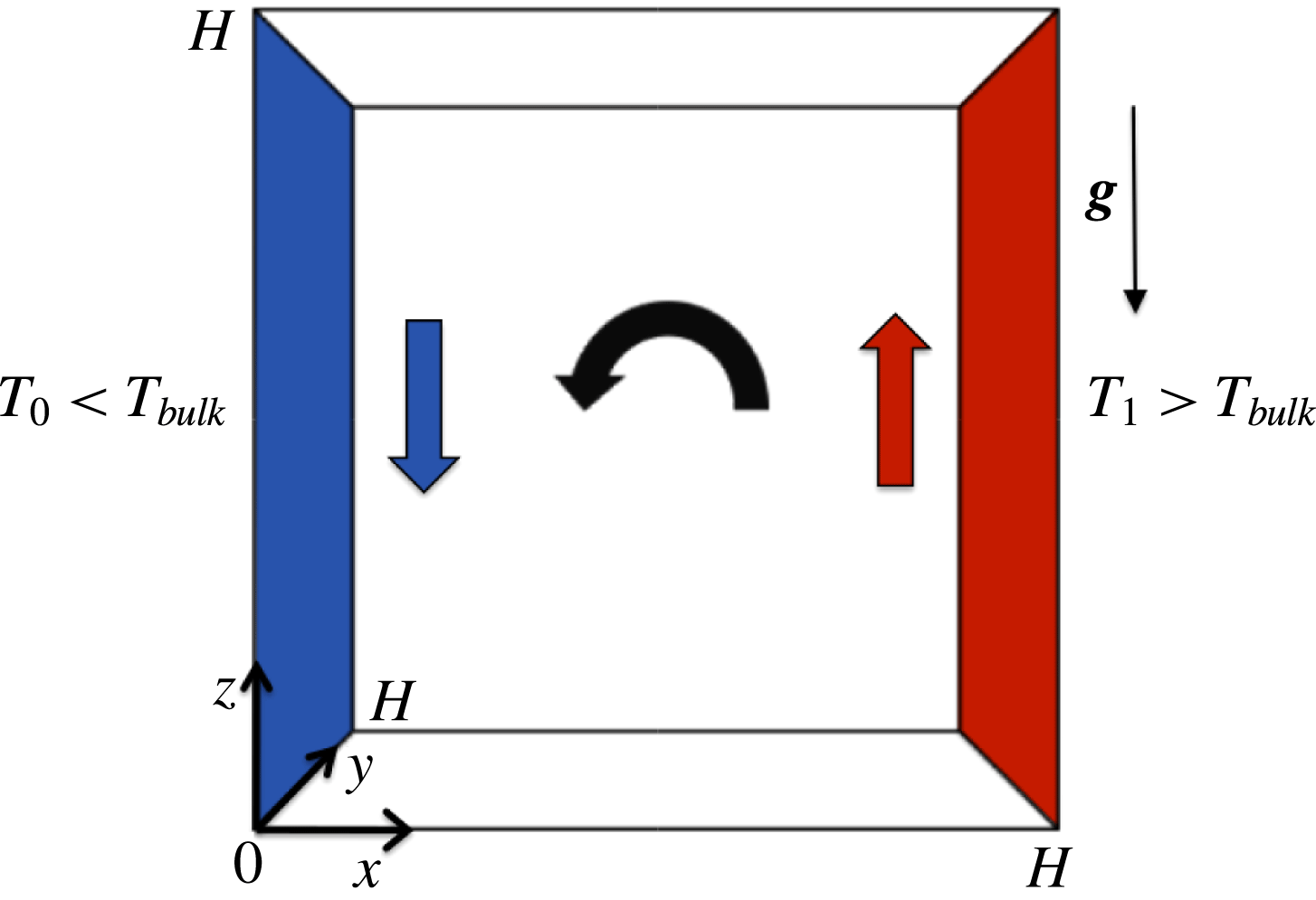
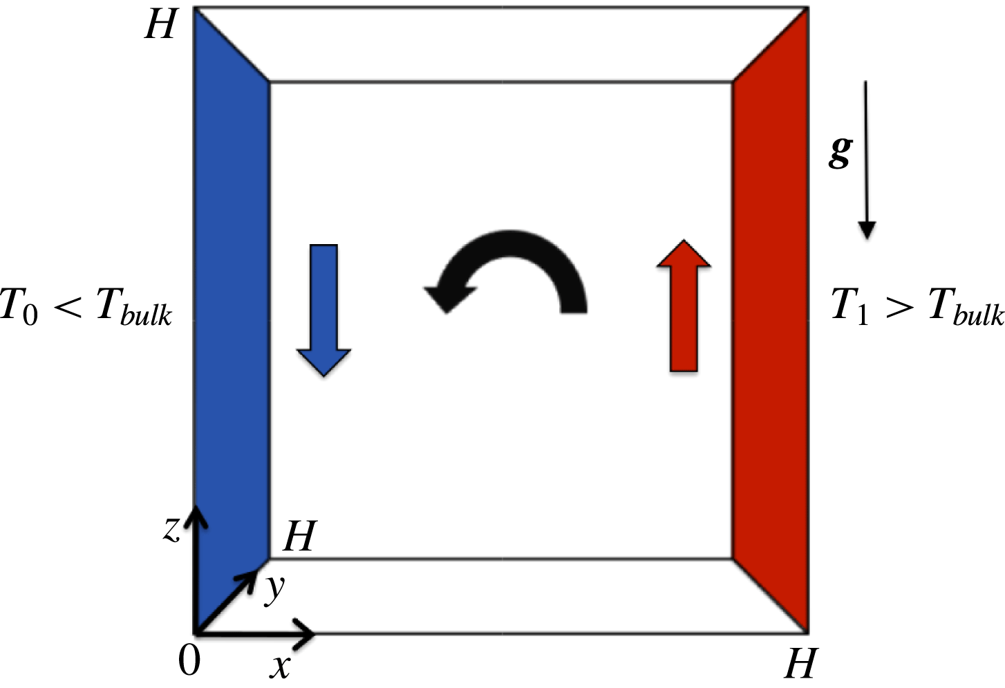
We consider the steady flow inside a cubical cavity (side length $H$ ) driven by buoyancy due to differential heating by two opposite vertical sidewalls at different temperature. The origin of the frame of reference is located in a corner of the cavity and gravity acts in the negative $z$ -direction as per figure 1. The fluid motion is driven by differential heating via the cold vertical wall at $x=0$ (temperature $T_{0}<T_{bulk}$ ) and the hot vertical wall $x=H$ (temperature $T_{1}>T_{bulk}$ ); the other walls are thermally insulated ( $\unicode[STIX]{x2202}T/\unicode[STIX]{x2202}n=0$ , with $n$ the wall normal). This sets up a circulatory flow due to rising and descending fluid at the hot and cold walls, respectively, as indicated schematically in figure 1. Furthermore, all walls are rigid and stationary, imposing no-slip conditions on the velocity ( $\boldsymbol{u}=\mathbf{0}$ ).

Figure 1.

Buoyancy-driven flow inside a cubical cavity due to differential heating via cold (blue; temperature $T_{0}<T_{bulk}$ ) and hot (red; $T_{1}>T_{bulk}$ ) vertical walls (perspective view into 3D cavity along $y$ -axis). Other walls are thermally insulated. This sets up circulatory flow (black arrow) due to rising (red arrow) and descending (blue arrow) fluid at hot and cold walls, respectively.

A Newtonian fluid with a velocity $\boldsymbol{u}$ governed by the steady Boussinesq equations

(2.1a-c ) $$\begin{eqnarray}\displaystyle \unicode[STIX]{x1D735}\boldsymbol{\cdot }\boldsymbol{u}=0,\quad \unicode[STIX]{x1D70C}\boldsymbol{u}\boldsymbol{\cdot }\unicode[STIX]{x1D735}\boldsymbol{u}=-\unicode[STIX]{x1D735}p+\unicode[STIX]{x1D707}\unicode[STIX]{x1D6FB}^{2}\boldsymbol{u}+\unicode[STIX]{x1D70C}\unicode[STIX]{x1D6FD}g(T-T_{ref})\boldsymbol{e}_{z},\quad \boldsymbol{u}\boldsymbol{\cdot }\unicode[STIX]{x1D735}T=\unicode[STIX]{x1D6FC}\unicode[STIX]{x1D6FB}^{2}T,\qquad \quad & & \displaystyle\end{eqnarray}$$

is assumed, where $T$ , $p$ and $\unicode[STIX]{x1D70C}$ are temperature, pressure and density, respectively, $T_{ref}$ the reference temperature for the fluid properties (here $T_{ref}=T_{0}$ ), $g$ the gravitational acceleration, $\boldsymbol{e}_{z}$ the $z$ -wise unit vector, $\unicode[STIX]{x1D707}$ the dynamic viscosity, $\unicode[STIX]{x1D6FD}$ the thermal expansion coefficient and $\unicode[STIX]{x1D6FC}$ the thermal diffusivity (Bird, Stewart & Lightfoot Reference Bird, Stewart and Lightfoot2007; Lappa Reference Lappa2010).

The Lagrangian motion of tracers passively advected by the velocity field $\boldsymbol{u}$ is governed by the kinematic equation and its corresponding (formal) solution

(2.2a,b ) $$\begin{eqnarray}\displaystyle \frac{\text{d}\boldsymbol{x}}{\text{d}t}=\boldsymbol{u}(\boldsymbol{x}),\quad \boldsymbol{x}(t)=\unicode[STIX]{x1D731}_{t}(\boldsymbol{x}_{0}), & & \displaystyle\end{eqnarray}$$

with $\boldsymbol{x}(t)$ and $\boldsymbol{x}_{0}$ the current and initial tracer positions, respectively, and $\unicode[STIX]{x1D731}_{t}$ the corresponding flow (Aref Reference Aref2002). Curves $\boldsymbol{x}(t)$ parameterised by $t$ describe the Lagrangian fluid trajectories, and in the current steady case coincide with the streamlines of the flow.

2.2 Non-dimensional formulation

The problem defined above will for reasons of universality be investigated in non-dimensional form. Non-dimensionalisation relies the scaling $\boldsymbol{x}=H\boldsymbol{x}^{\prime }$ , $\boldsymbol{u}=U\boldsymbol{u}^{\prime }$ , $p=Pp^{\prime }$ and $T=T_{0}+\unicode[STIX]{x0394}TT^{\prime }$ , with $U=g\unicode[STIX]{x1D6FD}\unicode[STIX]{x0394}TH^{2}/\unicode[STIX]{x1D708}$ , $P=\unicode[STIX]{x1D707}U/H$ , $H$ as before and $\unicode[STIX]{x0394}T=T_{1}-T_{0}$ the global temperature drop. Substitution in (2.1) and rearrangement (after dropping primes) yields

(2.3a-c ) $$\begin{eqnarray}\displaystyle \unicode[STIX]{x1D735}\boldsymbol{\cdot }\boldsymbol{u}=0,\quad Gr\boldsymbol{u}\boldsymbol{\cdot }\unicode[STIX]{x1D735}\boldsymbol{u}=-\unicode[STIX]{x1D735}p+\unicode[STIX]{x1D6FB}^{2}\boldsymbol{u}+T\boldsymbol{e}_{z},\quad GrPr\boldsymbol{u}\boldsymbol{\cdot }\unicode[STIX]{x1D735}T=\unicode[STIX]{x1D6FB}^{2}T, & & \displaystyle\end{eqnarray}$$

as non-dimensional Boussinesq approximation, parameterised by the Prandtl number $Pr=\unicode[STIX]{x1D708}/\unicode[STIX]{x1D6FC}$ and Grashof number $Gr=g\unicode[STIX]{x1D6FD}\unicode[STIX]{x0394}TH^{3}/\unicode[STIX]{x1D708}^{2}$ , where $\unicode[STIX]{x1D708}=\unicode[STIX]{x1D707}/\unicode[STIX]{x1D70C}$ is the kinematic viscosity. Thus the problem translates into a differentially heated cavity with unit side length and thermal boundary conditions $T=0$ at $x=0$ and $T=1$ at $x=1$ .

Non-dimensional form (2.3) concerns specifically the present regime of interest, viz. steady buoyancy-driven flow at strongly laminar conditions, implying a flow dominated by a balance between buoyancy (driving force) and viscous friction (restoring force), and thus the above characteristic velocity $U$ (Ostrach Reference Ostrach1988). This flow regime, given $Gr=UH/\unicode[STIX]{x1D708}=Re$ (Reynolds number), typically restricts the system to ‘lower’ $Gr$ .

The non-dimensional kinematic equation follows from scaling time as $t=\unicode[STIX]{x1D70F}t^{\prime }$ , with $\unicode[STIX]{x1D70F}=H/U$ the advective time scale, yielding a form identical to (2.2).

2.3 Numerical methods

The velocity and temperature fields governed by (2.3) were simulated by the commercial CFD package COMSOL Multiphysics using the Laminar Flow and Heat Transfer in Fluids modules with standard settings. The computational mesh consisted of $O(10^{5})$ elements and employed mesh refinement near the isothermal walls ( $x=0,1$ ). The tolerance factor for the nonlinear solver was set to yield residuals of $O(10^{-10}-10^{-12})$ .

The Lagrangian fluid trajectories are determined by numerical integration of the kinematic equation (2.2) using an explicit third-order Taylor–Galerkin (TG) scheme with adaptive step size (Speetjens, Clercx & van Heijst Reference Speetjens, Clercx and van Heijst2006; Moharana et al. Reference Moharana, Speetjens, Trieling and Clercx2013). Critical for reliable Lagrangian tracking is accurate approximation of the incompressibility constraint $\unicode[STIX]{x1D735}\boldsymbol{\cdot }\boldsymbol{u}=0$ at any position $\boldsymbol{x}$ in the flow domain. However, the degree of accuracy of commercial CFD packages in combination with the typical error propagation of standard spatial interpolation schemes for evaluation of the velocity in arbitrary positions generically introduces departures from incompressibility that may lead to numerical artefacts in the Lagrangian fluid trajectories. Thus an approach that ensures accurate approximation of the incompressibility constraint at any position $\boldsymbol{x}$ is essential. Consider to this end the dramatic difference in performance of the above TG scheme using standard interpolation of the velocity field of a typical commercial flow solver versus a dedicated flow solver and interpolation scheme for Lagrangian analyses based on a high-precision spectral method (Speetjens & Clercx Reference Speetjens and Clercx2005). The present study adopts a similar spectral approach by projection of the COMSOL field onto a divergence-free basis constructed from Chebyshev polynomials according to the method in § A.1. Performance of the TG tracking scheme using this spectral representation of the velocity field is evaluated in § A.2 and reveals reliable simulation of the Lagrangian dynamics.

Figure 2.

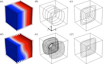
Temperature field (a,d) and typical streamlines (b,e, c,f) in limit $Gr=0$ (a–c) versus general case $Gr>0$ (d–f; $Gr=3.2\times 10^{3}$ ) demonstrated for $Pr=0.71$ . Blue/red in (a,d) indicates minimum/maximum temperatures; (c,f) gives streamlines in midplane $y=1/2$ . The dot in panel (b) indicates the origin of the shown reference frame.

3.1 Fundamental states of the Lagrangian flow topology

Non-dimensional form (2.3) admits identification of two fundamental flow states that are relevant in the context of the transport phenomena.

1. (i) Limit  $Gr=0$ . Here system (2.3) collapses on the linear Stokes limit $-\unicode[STIX]{x1D735}p+\unicode[STIX]{x1D6FB}^{2}\boldsymbol{u}+T\boldsymbol{e}_{z}=0$ and the conductive limit $\unicode[STIX]{x1D6FB}^{2}T=0$ .

2. (ii) General case  $Gr>0$ . The convective terms in the momentum and energy balances become relevant and render the system essentially nonlinear.

Figure 2 illustrates the essential features of both states in terms of temperature field and typical streamlines for $Pr=0.71$ . Figure 2(a–c) demonstrate the convergence on a linear temperature field and closed streamlines for vanishing $Gr$ . Here fluid motion consists solely of a primary circulation along these streamlines. Figure 2(d–f) demonstrate the essentially nonlinear temperature field and non-closed streamlines associated with departures from the limit $Gr=0$ by way of $Gr=3.2\times 10^{3}$ . Streamlines outside midplane $y=1/2$ describe toroidal structures as shown in figure 2(e) and cause fluid parcels, besides said primary circulation, to perform an additional secondary circulation about the common centre (not shown) of these tori; the streamlines in the midplane emerge from a central stagnation point (not shown) and spiral outward towards the cavity walls (figure 2 f). The behaviour of this stagnation point is key to the global Lagrangian dynamics and is investigated in detail in § 4.3. Moreover, the generic emergence of the above topological states as a function of $Gr$ is inextricably linked to symmetry properties and the Hamiltonian structure of the Lagrangian equations of motion. The former and latter will be investigated in §§ 3.2 and 3.4, respectively.

The above transition from linear temperature distributions and closed streamlines to nonlinear temperature fields and toroidal structures upon increasing $Gr$ from the limit $Gr=0$ is generic for any fluid and thus (qualitatively) independent of $Pr$ here. However, in order to nonetheless explore the (quantitative) role of $Pr$ , the Lagrangian dynamics in buoyancy-driven flows is in the present study demonstrated and investigated mainly by way of two specific cases, viz. air ( $Pr=0.71$ ) and water ( $Pr=7$ ). This is motivated by their great practical relevance and prominence in the literature (de Vahl Davis Reference de Vahl Davis1983; Melnikov & Shevtsova Reference Melnikov and Shevtsova2005; Lappa Reference Lappa2010; Oteski et al. Reference Oteski, Duguet, Pastur and Le Quéré2015; Contreras et al. Reference Contreras, Speetjens and Clercx2016b ).

3.2 Symmetry analysis

Symmetries are key organising mechanisms of the Lagrangian flow topology and typically originate from an interplay between symmetries in geometry and governing equations (Laure Reference Laure1987; Franjione & Ottino Reference Franjione and Ottino1992; Speetjens, Clercx & van Heijst Reference Speetjens, Clercx and van Heijst2004; Speetjens et al. Reference Speetjens, Demissie, Metcalfe and Clercx2014). Relevant in the present context is that the buoyancy term in the momentum equation admits a Helmholtz decomposition (Arfken & Weber Reference Arfken and Weber2005) into an irrotational and solenoidal part as $T\boldsymbol{e}_{z}=\unicode[STIX]{x1D735}\unicode[STIX]{x1D719}+\unicode[STIX]{x1D735}\times \boldsymbol{b}$ , with $\unicode[STIX]{x1D735}\unicode[STIX]{x1D719}=\widetilde{T}\boldsymbol{e}_{z}$ and $\unicode[STIX]{x1D735}\times \boldsymbol{b}=\widehat{T}\boldsymbol{e}_{z}$ , where $\widetilde{T}=1/2$ and $\widehat{T}=T-1/2$ . (Note that $-1/2\leqslant \widehat{T}\leqslant 1/2$ .) This gives $\unicode[STIX]{x1D719}=z/2$ , which merely adjusts the pressure (i.e. $p\rightarrow \widehat{p}=p-\unicode[STIX]{x1D719}$ in (2.3)), exposing $\widehat{T}\boldsymbol{e}_{z}$ as the effective buoyancy force.

Velocity $\boldsymbol{u}$ and temperature contribution $\widehat{T}$ possess the following symmetries for buoyancy-driven flow in rectangular cavities in the general case $Gr>0$ (Laure Reference Laure1987).

1. (i) Reflectional symmetry about plane $y=1/2$ (denoted ${\mathcal{P}}$ hereafter):

   (3.1a,b ) $$\begin{eqnarray}\displaystyle \boldsymbol{S}_{i}:(x,y,z)\rightarrow (x,1-y,z),\quad (u_{x},u_{y},u_{z},\widehat{T})\rightarrow (u_{x},-u_{y},u_{z},\widehat{T}). & & \displaystyle\end{eqnarray}$$

2. (ii) Centro-symmetry about line $x=z=1/2$ (denoted ${\mathcal{L}}$ hereafter):

   (3.2a,b ) $$\begin{eqnarray}\displaystyle \boldsymbol{S}_{ii}:(x,y,z)\rightarrow (1-x,y,1-z),\quad (u_{x},u_{y},u_{z},\widehat{T})\rightarrow (-u_{x},u_{y},-u_{z},-\widehat{T}).\qquad & & \displaystyle\end{eqnarray}$$

Numerous computational studies confirm symmetries (3.1) and (3.2) (Labrosse et al. Reference Labrosse, Tric, Khallouf and Betrouni1997; Henry & Buffat Reference Henry and Buffat1998; Juel et al. Reference Juel, Mullin, Ben Hadid and Henry1999; Wakashima & Saitoh Reference Wakashima and Saitoh2004; Bennett et al. Reference Bennett, Anne and Hsueh2006; Henry et al. Reference Henry, Juel, Ben Hadid and Kaddeche2008).

Centro-symmetry (3.2) in the limit $Gr=0$ divides into the reflectional symmetry

(3.3a,b ) $$\begin{eqnarray}\displaystyle \boldsymbol{S}_{ii,x}:(x,y,z)\rightarrow (1-x,y,z),\quad (u_{x},u_{y},u_{z},\widehat{T})\rightarrow (u_{x},-u_{y},-u_{z},-\widehat{T}), & & \displaystyle\end{eqnarray}$$

about plane $x=1/2$ and the reflectional symmetry

(3.4a,b ) $$\begin{eqnarray}\displaystyle \boldsymbol{S}_{ii,z}:(x,y,z)\rightarrow (x,y,1-z),\quad (u_{x},u_{y},u_{z},\widehat{T})\rightarrow (-u_{x},-u_{y},u_{z},\widehat{T}), & & \displaystyle\end{eqnarray}$$

about plane $z=1/2$ . Note that the symmetries relate via $\boldsymbol{S}_{ii}=\boldsymbol{S}_{ii,x}\boldsymbol{S}_{ii,z}=\boldsymbol{S}_{ii,z}\boldsymbol{S}_{ii,x}$ . Symmetries (3.3) and (3.4) emerge on grounds of vanishing inertial and convective terms in (2.3) in the limit $Gr=0$ . Inertia and/or convective heat transfer induced by appreciable $Gr>0$ breaks these symmetries in favour of symmetry (3.2). Hence, cases $Gr=0$ and $Gr>0$ are essentially distinct and underlie the fundamental topological states identified in § 3.1. This is elaborated below.

Symmetry (3.1), commonly denoted ‘left–right symmetry’ in convection problems, exists for any $Gr$ and separates the domain into two subregions by ${\mathcal{P}}$ . The latter, since $u_{y}=0$ due to the anti-symmetry of $u_{y}$ , constitutes an invariant material plane bounded by the cavity walls. This has two immediate topological consequences. First, Lagrangian entities are either restricted to ${\mathcal{P}}$ or emerge as symmetric pairs about this plane. Second, midplane ${\mathcal{P}}$ must, by virtue of Brouwer’s fixed-point theorem (Brouwer Reference Brouwer1911), hold at least one stagnation point $\boldsymbol{u}=\mathbf{0}$ .

The fundamental flow states of § 3.1 emanate from the above symmetries as follows.

1. (i) Limit  $Gr=0$ . The primary circulation causes streamlines to generically cross the symmetry plane $x=1/2$ of reflectional symmetry (3.3). (This ignores possible corner eddies (Shankar Reference Shankar1997); these are very weak and highly localised and thus irrelevant to the overall Lagrangian dynamics.) This has the fundamental implication that such streamlines must be closed (Shankar Reference Shankar1997). Note that symmetry (3.4) has the same effect. Moreover, interaction of symmetries (3.1), (3.3) and (3.4) results in the formation of a stagnation line $x=z=1/2$ . Hence, the Lagrangian flow topology generically consists of closed streamlines centred on said stagnation line that individually exhibit reflectional symmetry about both planes $x=1/2$ and $z=1/2$ and emerge in symmetric pairs about ${\mathcal{P}}$ (as demonstrated in figure 2 b).

2. (ii) General case  $Gr>0$ . Breakdown of reflectional symmetries (3.3) and (3.4) in favour of centro-symmetry (3.2) eliminates the constraining mechanism underlying the formation of closed streamlines. Hence, streamlines generically become non-closed in this regime. Moreover, the stagnation line gives way to an isolated stagnation point $\boldsymbol{x}_{c}=(1/2,1/2,1/2)$ in the centre of the cavity, which results from the interaction of symmetries (3.1) and (3.2). 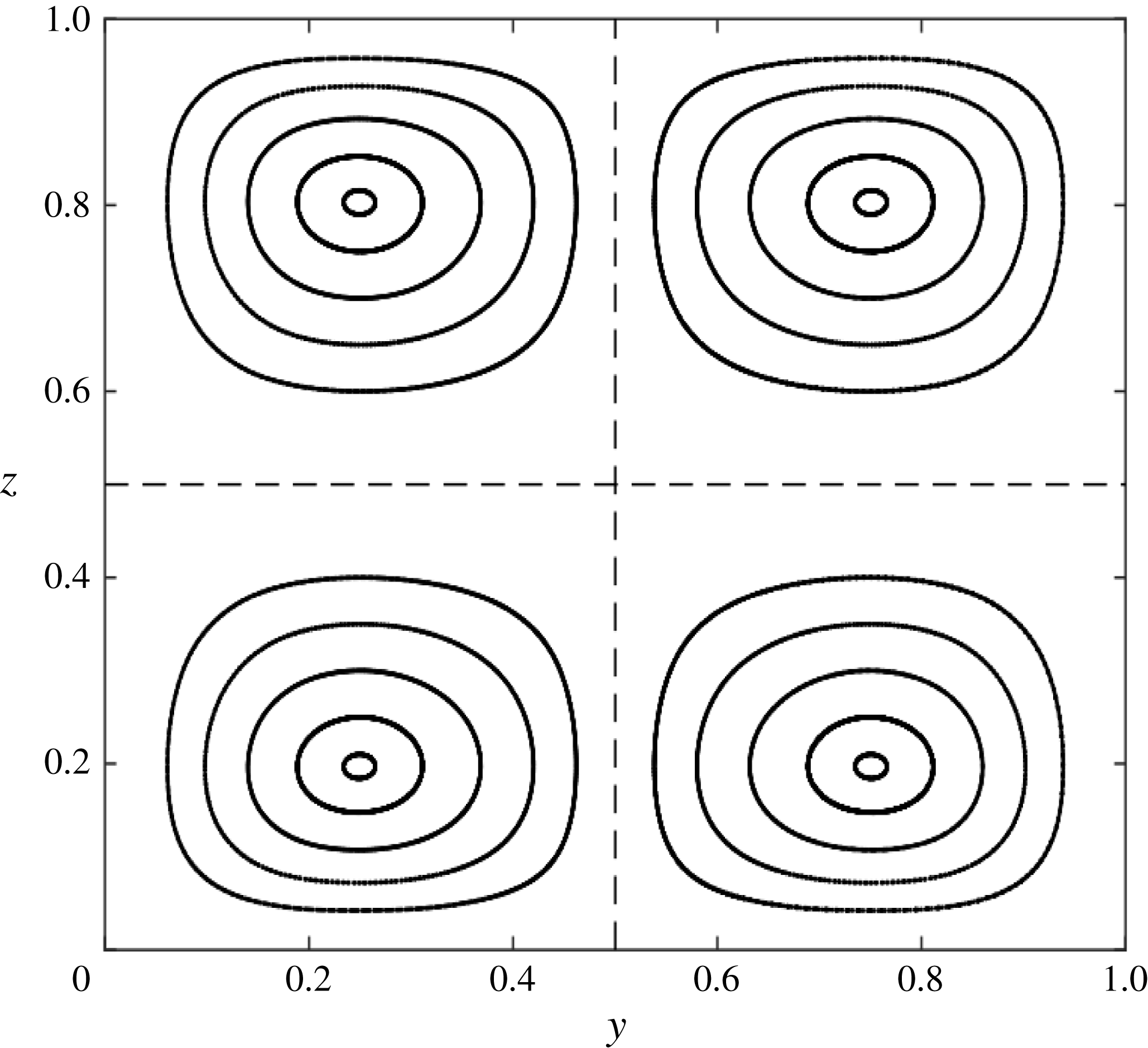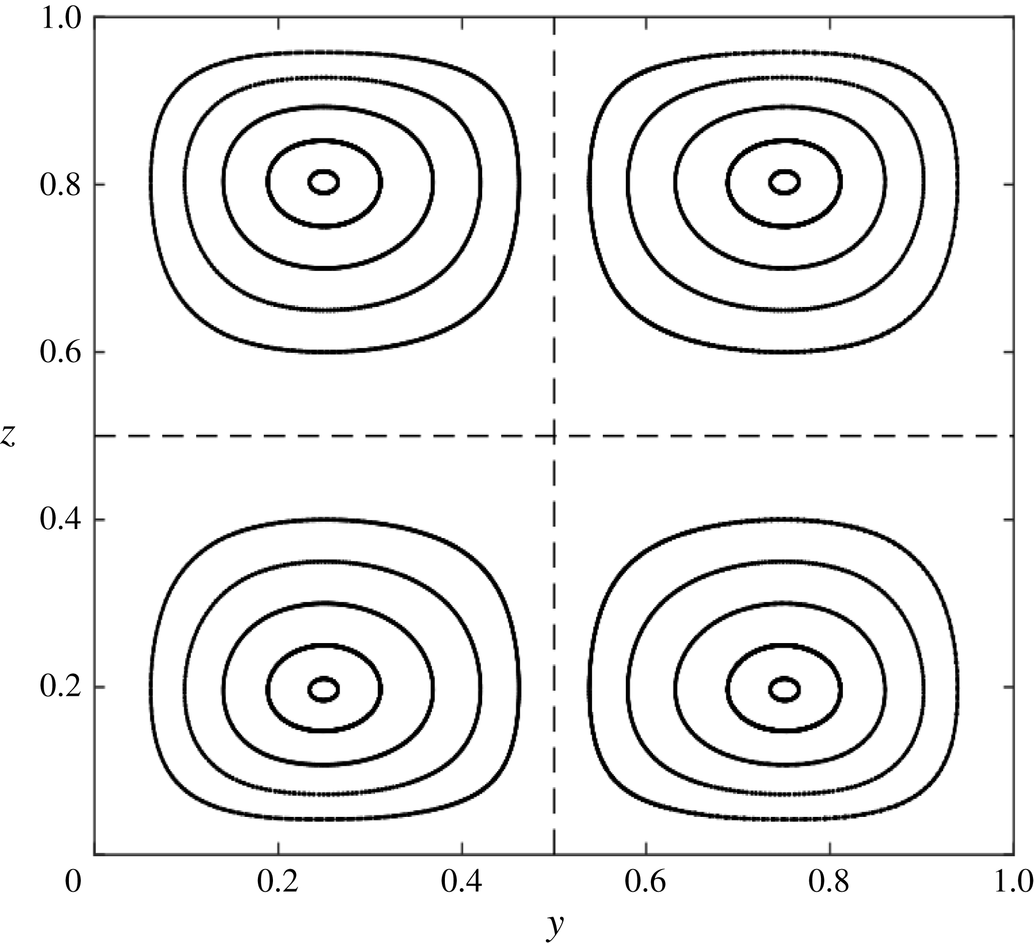Thus the Lagrangian flow topology generically consists of non-closed streamlines that each describe toroidal structures arranged symmetrically about ${\mathcal{P}}$ in the way demonstrated in figure 2(e). Figure 3 gives the corresponding intersections with plane $x=1/2$ for $Gr=7.9\times 10^{2}$ and thus exposes these toroidal structures. Note that $\boldsymbol{S}_{ii}$ implies a reflectional symmetry about lines $z=1/2$ and $x=1/2$ within the planes $x=1/2$ and $z=1/2$ , respectively. This causes the symmetry of shown cross-sections with plane $x=1/2$ about both lines $y=1/2$ and $z=1/2$ (dashed in figure 3) and a similar symmetry in plane $z=1/2$ about lines $x=1/2$ and $y=1/2$ .

The above rigorously links the generic topological make-up of the 3D streamline portrait to symmetries, which is key to the present study. Symmetries namely ‘shape’ the fundamental topological states identified in § 3.1. Moreover, the particular way in which symmetries are broken dictates the response of the flow topology and, inherently, the Lagrangian transport properties to perturbations. Symmetry and symmetry breaking (investigated in § 4) are controlled primarily by the Grashof number $Gr$ , and thus underscores the crucial role of this parameter for the Lagrangian dynamics.

Figure 3.

Formation of toroidal structures by non-closed streamlines in the generic case $Gr>0$ demonstrated for $Gr=7.9\times 10^{2}$ and $Pr=0.71$ . Shown are cross-sections with the plane $x=1/2$ ; these are always symmetric about lines $y=1/2$ and $z=1/2$ (dashed).

3.3 Topological equivalence with single-wall lid-driven cavity flows

The above symmetries establish a fundamental link between the buoyancy-driven flow and lid-driven cavity flows. Fluid motion in cylindrical or cubical domains driven by a single endwall $z=0$ or $z=H$ in the Stokes limit ( $Re=0$ ) namely possess the same symmetries (3.1) and (3.3) and, in consequence, their flow topology also consists of closed streamlines centred on a stagnation line symmetric about ${\mathcal{P}}$ similar to in figure 2(b) (Shankar Reference Shankar1997; Shankar & Deshpande Reference Shankar and Deshpande2000; Speetjens et al. Reference Speetjens, Clercx and van Heijst2004). A counterpart to symmetry (3.4) is absent in single-wall lid-driven Stokes flows ( $Re=0$ ) yet this is, other than admitting asymmetry about the plane $z=1/2$ , inconsequential for the topological equivalence with the buoyancy-driven flow (limit $Gr=0$ ). The equivalence extends to lid-driven flows with fluid inertia ( $Re>0$ ) in that, similar to case $Gr>0$ , symmetry (3.3) is broken, causing streamlines to generically become non-closed and describe toroidal structures similar to in figure 2(e) (Shankar & Deshpande Reference Shankar and Deshpande2000; Speetjens et al. Reference Speetjens, Clercx and van Heijst2006; Speetjens & Clercx Reference Speetjens, Clercx and Klapp2013). Absence of a counterpart to centro-symmetry (3.2) is again immaterial for the topological equivalence. Note that buoyancy-induced topological bifurcations may complicate (yet not eliminate) the equivalence (§ 4).

The topological equivalence between buoyancy-driven and lid-driven cavity flows implies a second fundamental link for these flow classes: the Lagrangian equations of motion (2.2) have a Hamiltonian structure. This has the important consequence that the response of the flow topology to departures from limit $Gr=0$ is governed by the same universal Hamiltonian mechanisms as in single-wall lid-driven flows. The Hamiltonian structure and its ramifications for the Lagrangian dynamics are elaborated below.

3.4 Formation of the flow topology by Hamiltonian mechanisms

The primary circulation causes (similar to lid-driven flows) systematic return of generic streamlines to plane $x=1/2$ . This admits representation of the 3D flow $\boldsymbol{x}(t)=\unicode[STIX]{x1D731}_{t}(\boldsymbol{x}_{0})$ governed by kinematic equation (2.2) by a 2D map $\unicode[STIX]{x1D731}$ within plane $x=1/2$ according to

(3.5) $$\begin{eqnarray}\displaystyle \boldsymbol{x}_{k+1}=\unicode[STIX]{x1D731}(\boldsymbol{x}_{k}), & & \displaystyle\end{eqnarray}$$

with $\boldsymbol{x}_{k}=(y_{k},z_{k})$ the $k$ th intersection of a 3D streamline originating from $\boldsymbol{x}_{0}$ with said plane (appendix B). The sequence of planar positions of a given fluid parcel, i.e.

(3.6) $$\begin{eqnarray}\displaystyle {\mathcal{X}}(\boldsymbol{x}_{0})=\{\boldsymbol{x}_{0},\boldsymbol{x}_{1},\ldots ,\boldsymbol{x}_{k},\ldots \}, & & \displaystyle\end{eqnarray}$$

represents the subsequent intersections of its corresponding 3D streamline with plane $x=1/2$ and constitutes its so-called Poincaré section. Coherent structures in the Poincaré section are inextricably linked to those in the 3D streamline portrait. Closed streamlines, for example, emerge as periodic points $\unicode[STIX]{x1D731}^{p}(\boldsymbol{x}_{0})=\boldsymbol{x}_{0}$ , with $p$ the winding number of the streamline, in the corresponding Poincaré section. Similarly, 3D toroidal structures appear as ‘islands’ centred on periodic points in these sections; figure 3, for example, shows the Poincaré section of such tori for $Gr=7.9\times 10^{2}$ and $Pr=0.71$ (which are similar to those in figure 2 e). Thus map $\unicode[STIX]{x1D731}$ enables investigation of the flow topology both in terms of the dynamics within plane $x=1/2$ and 3D streamlines.

Map $\unicode[STIX]{x1D731}$ , in turn, through a suitable transformation from physical $(y,z)$ to canonical ( $\unicode[STIX]{x1D701}_{1},\unicode[STIX]{x1D701}_{2}$ ) space coincides with a 2D Hamiltonian system, i.e.

(3.7) $$\begin{eqnarray}\displaystyle \boldsymbol{x}_{k+1}=\unicode[STIX]{x1D731}(\boldsymbol{x}_{k})\quad \Leftrightarrow \quad \left(\frac{\text{d}\unicode[STIX]{x1D701}_{1}}{\text{d}\unicode[STIX]{x1D70F}},\frac{\text{d}\unicode[STIX]{x1D701}_{2}}{\text{d}\unicode[STIX]{x1D70F}}\right)=\left(\frac{\unicode[STIX]{x2202}{\mathcal{H}}}{\unicode[STIX]{x2202}\unicode[STIX]{x1D701}_{2}},-\frac{\unicode[STIX]{x2202}{\mathcal{H}}}{\unicode[STIX]{x2202}\unicode[STIX]{x1D701}_{1}}\right), & & \displaystyle\end{eqnarray}$$

with ${\mathcal{H}}$ the Hamiltonian. This ties the Lagrangian dynamics in plane $x=1/2$ described by map (3.5) with ‘snapshots’ in canonical time $\unicode[STIX]{x1D70F}$ of the Hamiltonian flow in canonical space ( $\unicode[STIX]{x1D701}_{1},\unicode[STIX]{x1D701}_{2}$ ). Consult appendix B for technical details.

The link with Hamiltonian systems established above implies that the flow topology is governed by Hamiltonian mechanics. The behaviour of Hamiltonian systems emanates from the perturbation of the so-called integrable states (in essence states with fully regular dynamics along closed trajectories in phase space) (Ott Reference Ott2002). For the present buoyancy-driven flows, the integrable state corresponds to the closed streamlines in the limit $Gr=0$ (as, for example, in figure 2 b). Perturbation by $Gr>0$ admits non-closed streamlines and thus sets the stage for non-trivial flow topologies (including chaotic dynamics). The onset of such flow topologies is governed by well-defined Hamiltonian scenarios and is here (qualitatively) controlled by the Grashof number $Gr$ as follows.

1. (i) Limit  $Gr=0$ . The underlying Hamiltonian system (3.7) assumes the integrable state, meaning its Hamiltonian becomes ${\mathcal{H}}(\unicode[STIX]{x1D701}_{1},\unicode[STIX]{x1D701}_{2},\unicode[STIX]{x1D70F})=C$ , with $C$ an arbitrary constant. Thus each individual position in the associated Poincaré section constitutes a period-1 point, i.e. $\unicode[STIX]{x1D731}(\boldsymbol{x}_{k})=\boldsymbol{x}_{k}$ , consistent with the situation of all streamlines being individually closed (e.g. figure 2 b). This state in fact is a singular limit in that it breaks down for any non-zero perturbation (Cartwright, Feingold & Piro Reference Cartwright, Feingold and Piro1996). (Limit $Gr=0$ is singular also in the sense of implying vanishing dimensional flow due to scaling $U=Gr\unicode[STIX]{x1D708}/H$ ( $=0$ here). However, the corresponding non-dimensional flow is non-trivial and constitutes a non-inertial fluid driven by a symmetric buoyancy term resulting from a linear temperature profile governed by conductive heat transfer only. Hence, case $Gr=0$ , though strictly with trivial dimensional counterpart, is nonetheless relevant in the current Lagrangian context as the (theoretical) limit of fully integrable Lagrangian dynamics.)

2. (ii) ‘Small’  $Gr$ . Minute (non-zero) perturbations of $O(\unicode[STIX]{x1D716})$ , with $\unicode[STIX]{x1D716}\ll 1$ , cause the Hamiltonian to become non-trivial yet remain independent of the canonical time $\unicode[STIX]{x1D70F}$ : ${\mathcal{H}}={\mathcal{H}}(\unicode[STIX]{x1D701}_{1},\unicode[STIX]{x1D701}_{2})$ (Cartwright et al. Reference Cartwright, Feingold and Piro1996). (‘Small’ and ‘large’ $Gr$ are distinguished by the corresponding typical perturbation $\unicode[STIX]{x1D716}$ .) This defines an autonomous 2D Hamiltonian system with Lagrangian motion (in bounded flows) restricted to concentric closed level sets of ${\mathcal{H}}$ in the Poincaré section (e.g. the islands in figure 3). These level sets underlie the nested tori that form in the 3D streamline portrait (e.g. figure 2 e). The $\unicode[STIX]{x1D70F}$ -dependence vanishes due to the fact that, since the primary circulation is much faster compared to the secondary circulation, the dynamics only ‘feel’ the averaged perturbation in (canonical) time $\unicode[STIX]{x1D70F}$ . This is known as ‘averaging’ and is a generic phenomenon in dynamical systems leading to the formation of invariant manifolds (here tori) (Arnol’d Reference Arnol’d1989). This averaging effect is independent of the particular nature of the perturbations (provided they are weak), thus explaining the observations in Contreras et al. (Reference Contreras, Speetjens and Clercx2016b ) that (weak) fluid inertia as well as convective heat transfer may trigger this behaviour.

3. (iii) ‘Large’  $Gr$ . Here perturbations exceed $O(\unicode[STIX]{x1D716})$ and the Hamiltonian becomes dependent on canonical time $\unicode[STIX]{x1D70F}$ , i.e. ${\mathcal{H}}={\mathcal{H}}(\unicode[STIX]{x1D701}_{1},\unicode[STIX]{x1D701}_{2},\unicode[STIX]{x1D70F})$ , rendering system (3.7) non-autonomous and, generically, non-integrable (Ott Reference Ott2002). This has fundamental consequences for the flow topology in that some tori disintegrate and (locally) give way to chaotic dynamics while other tori survive and constitute transport barriers. Tori associated with rational streamlines (i.e. emerging as periodic points $\unicode[STIX]{x1D731}^{p}(\boldsymbol{x}_{k})=\boldsymbol{x}_{k}$ in the Poincaré section for some finite periodicity $p$ ) disintegrate into the characteristic island chains surrounded by chaotic regions; tori associated with irrational streamlines (i.e. describing complete concentric curves in said Poincaré section) survive and thus form transport barriers. The fate of the rational and irrational tori in 2D Hamiltonian systems is respectively described by the well-known Poincaré–Birkhoff and KAM theorems (Ott Reference Ott2002); counterparts of these ‘classical’ theorems for the current 3D steady flows are given in, for example, Cheng & Sun (Reference Cheng and Sun1990a ,Reference Cheng and Sun b ). The surviving tori are commonly denoted ‘KAM tori’ in literature.

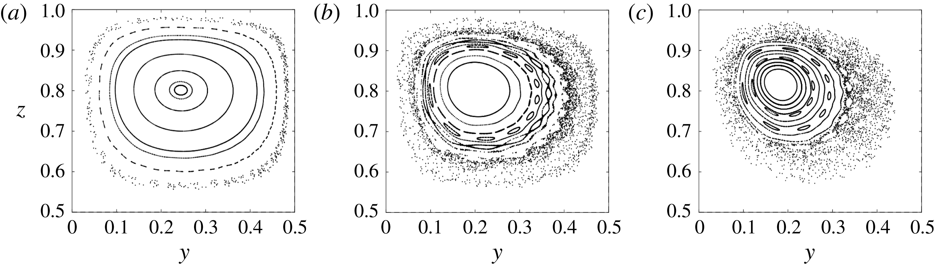
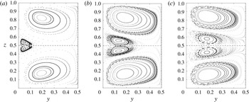
The generic response scenario of the flow topology to increasing $Gr$ is demonstrated by the Poincaré section for the previous example $Pr=0.71$ in figure 4 (only upper-left quadrant $(y,z)\in [0,1/2]\times [1/2,1]$ is shown owing to symmetry within plane $x=1/2$ ). Case $Gr=3.2\times 10^{3}$ corresponds with the regime of ‘small’ $Gr$ characterised by the islands within the Poincaré section shown in figure 4(a). Note that ‘small’ and ‘large’ $Gr$ are distinguished by the corresponding typical perturbation strength and not by the value of $Gr$ itself; the correlation in general is case-specific (here the observed dynamics, for example, imply that $Gr=3.2\times 10^{3}$ yields a perturbation of $O(\unicode[STIX]{x1D716})$ ). Increasing $Gr$ triggers the response scenarios of the islands (and tori in 3D) associated with ‘large’ $Gr$ . 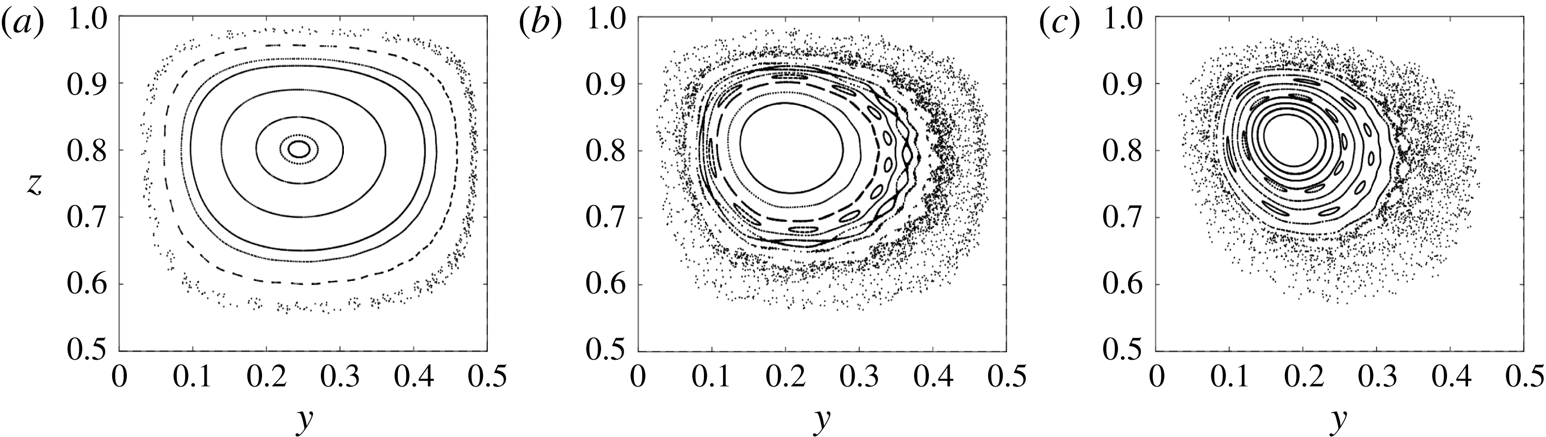Figure 4(b) reveals the emergence of an eleven-island chain at $Gr=2.4\times 10^{4}$ due to the breakdown of a rational torus surrounded by surviving islands (corresponding with KAM tori in 3D). Further increasing $Gr$ progressively triggers further torus breakdown, giving rise to the ‘classical’ Hamiltonian picture of KAM tori coexisting with island chains accompanied by (ever wider) chaotic bands, as demonstrated in figure 4(c) for $Gr=7.2\times 10^{4}$ .

Figure 4.

Hamiltonian breakdown of toroidal structures with increasing departure from the limit $Gr=0$ demonstrated for $Pr=0.71$ : (a) $Gr=3.2\times 10^{3}$ ; (b) $Gr=2.4\times 10^{4}$ ;(c) $Gr=7.2\times 10^{4}$ . Visualisation by intersections with the plane $x=1/2$ (‘Poincaré section’); only upper-left quadrant $(y,z)\in [0,1/2]\times [1/2,1]$ is shown owing to symmetry within plane $x=1/2$ .

The single-wall lid-driven flow (qualitatively) follows the same scenario upon perturbation by, for example, fluid inertia or asymmetric wall forcing (Shankar Reference Shankar1998; Speetjens et al. Reference Speetjens, Clercx and van Heijst2006; Ishii, Ota & Adachi Reference Ishii, Ota and Adachi2012; Speetjens & Clercx Reference Speetjens, Clercx and Klapp2013; Wu et al. Reference Wu, Speetjens, Vainchtein, Trieling and Clercx2014). This further substantiates their intimate dynamic similarity with the current buoyancy-driven flow and, as a consequence, the universality of the Lagrangian dynamics in 3D steady bounded flows. However, the current flow class admits a more elaborate interplay between fluid-dynamical forces due to, besides viscous and inertial forces, the presence of a third force: buoyancy. This may result in greater dynamic richness (as demonstrated and investigated in § 4).

4.1 First ‘stage’ of symmetry breaking: inertia-dominated dynamics

The nature of the stagnation point $\boldsymbol{x}_{c}=(1/2,1/2,1/2)$ is determined by the spectral properties of the strain-rate tensor $\unicode[STIX]{x1D641}=\unicode[STIX]{x2202}\boldsymbol{u}/\unicode[STIX]{x2202}\boldsymbol{x}|_{\boldsymbol{x}_{c}}$ (Guckenheimer & Holmes Reference Guckenheimer and Holmes1983; Chong, Perry & Cantwell Reference Chong, Perry and Cantwell1990). Symmetries (3.1) and (3.2) imply $\unicode[STIX]{x2202}u_{x}/\unicode[STIX]{x2202}y=\unicode[STIX]{x2202}u_{z}/\unicode[STIX]{x2202}y=0$ and $\unicode[STIX]{x2202}u_{y}/\unicode[STIX]{x2202}x=\unicode[STIX]{x2202}u_{y}/\unicode[STIX]{x2202}z=0$ , respectively, and in conjunction with incompressibility simplify $\unicode[STIX]{x1D641}$ to

(4.1a,b ) $$\begin{eqnarray}\displaystyle \unicode[STIX]{x1D641}=\left.\frac{\unicode[STIX]{x2202}\boldsymbol{u}}{\unicode[STIX]{x2202}\boldsymbol{x}}\right|_{\boldsymbol{x}_{c}}=\left[\begin{array}{@{}ccc@{}}\unicode[STIX]{x2202}u_{x}/\unicode[STIX]{x2202}x & 0 & \unicode[STIX]{x2202}u_{x}/\unicode[STIX]{x2202}z\\ 0 & -A & 0\\ \unicode[STIX]{x2202}u_{z}/\unicode[STIX]{x2202}x & 0 & \unicode[STIX]{x2202}u_{z}/\unicode[STIX]{x2202}z,\end{array}\right],\quad A=\frac{\unicode[STIX]{x2202}u_{x}}{\unicode[STIX]{x2202}x}+\frac{\unicode[STIX]{x2202}u_{z}}{\unicode[STIX]{x2202}z}, & & \displaystyle\end{eqnarray}$$

in $\boldsymbol{x}_{c}$ . This yields

(4.2a-c ) $$\begin{eqnarray}\displaystyle \unicode[STIX]{x1D706}_{1}=-A,\quad \unicode[STIX]{x1D706}_{2,3}=\frac{A}{2}\pm \sqrt{B},\quad B=\frac{1}{4}\left[\frac{\unicode[STIX]{x2202}u_{x}}{\unicode[STIX]{x2202}x}-\frac{\unicode[STIX]{x2202}u_{z}}{\unicode[STIX]{x2202}z}\right]^{2}+\frac{\unicode[STIX]{x2202}u_{x}}{\unicode[STIX]{x2202}z}\frac{\unicode[STIX]{x2202}u_{z}}{\unicode[STIX]{x2202}x}, & & \displaystyle\end{eqnarray}$$

as eigenvalue spectrum, which depends entirely on the planar velocity $(u_{x},u_{z})$ in the symmetry plane ${\mathcal{P}}$ . Moreover, it can be shown that the corresponding eigenvectors are of the form $\boldsymbol{v}_{1}=\boldsymbol{e}_{y}$ and $\boldsymbol{v}_{2,3}=\unicode[STIX]{x1D6FC}\boldsymbol{e}_{x}\pm \unicode[STIX]{x1D6FD}\boldsymbol{e}_{z}$ , signifying orientations normal and parallel, respectively, to said plane. The type of the stagnation point $\boldsymbol{x}_{c}$ is governed by $\text{sign}(B)$ and, adopting the nomenclature by Chong et al. (Reference Chong, Perry and Cantwell1990), for incompressible flows ( $\unicode[STIX]{x1D735}\boldsymbol{\cdot }\boldsymbol{u}=\unicode[STIX]{x1D706}_{1}+\unicode[STIX]{x1D706}_{2}+\unicode[STIX]{x1D706}_{3}=0$ ) admits two cases: (i) focus for $B<0$ (complex conjugate eigenvalues $\unicode[STIX]{x1D706}_{2,3}$ ); (ii) node/saddle/saddle (NSS) for $B>0$ (real eigenvalues $\unicode[STIX]{x1D706}_{2,3}$ ).

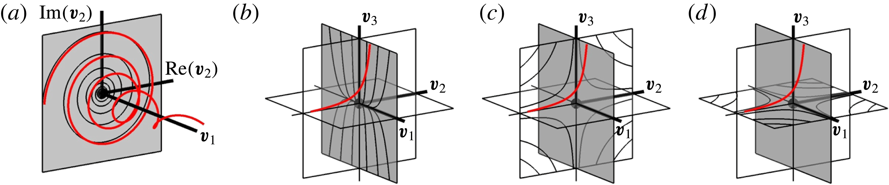
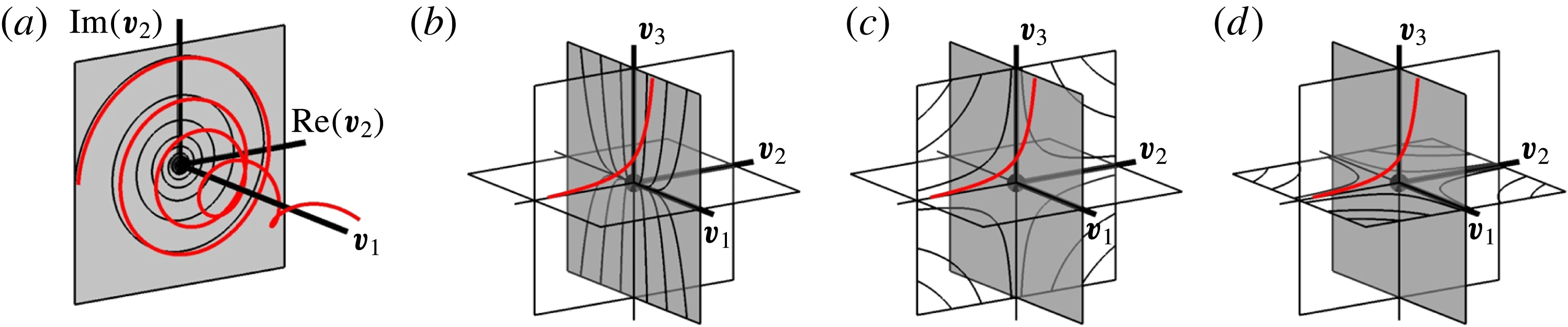
Figure 5(a) gives the flow topology near $\boldsymbol{x}_{c}$ (black marker) in case $\boldsymbol{x}_{c}$ being a focus including a typical streamline (red). Eigenvector $\boldsymbol{v}_{1}$ locally defines the corresponding 1D manifold $W_{1D}$ (heavy line) and normal of the 2D manifold $W_{2D}$ (shaded). Orientation $\boldsymbol{v}_{1}\in {\mathcal{L}}$ through the global symmetries according to § 3.2 then readily yields $W_{1D}={\mathcal{L}}$ and $W_{2D}={\mathcal{P}}$ for a focus-type $\boldsymbol{x}_{c}$ . The eigenvalue spectrum of a NSS-type $\boldsymbol{x}_{c}$ always comprises a pair of eigenvalues of equal sign and an isolated eigenvalue of opposite sign; the eigenvectors of former and latter locally define $W_{2D}$ and $W_{1D}$ , respectively. The streamline portrait within $W_{2D}$ corresponds with a node; the portrait in the two transverse canonical planes corresponds with a saddle. Figure 5(b–d) demonstrates this for the case $\text{sign}(\unicode[STIX]{x1D706}_{1})=\text{sign}(\unicode[STIX]{x1D706}_{3})=-\text{sign}(\unicode[STIX]{x1D706}_{2})$ , where $W_{2D}$ and $W_{1D}$ correspond with $(\boldsymbol{v}_{1},\boldsymbol{v}_{3})$ -plane (shaded) and $\boldsymbol{v}_{2}$ -axis, respectively, and red indicates a typical streamline. The streamline portraits within $W_{2D}$ (a) and the transverse $(\boldsymbol{v}_{2},\boldsymbol{v}_{3})$ -plane (b,c) and $(\boldsymbol{v}_{1},\boldsymbol{v}_{2})$ -plane (d) are shown separately for legibility. Note that figure 5(b–d) gives the sole manifold orientation possible for NSS-type $\boldsymbol{x}_{c}$ . This is discussed in § 4.2.

Figure 5.

Flow topology near stagnation point $\boldsymbol{x}_{c}$ (black marker) in canonical space spanned by eigenvectors $(\boldsymbol{v}_{1},\boldsymbol{v}_{2},\boldsymbol{v}_{3})$ including typical streamline (red): (a) focus with $W_{1D}$ (heavy line) and $W_{2D}$ (shaded); (b–d) NSS with here $W_{2D}$ and $W_{1D}$ corresponding with $(\boldsymbol{v}_{1},\boldsymbol{v}_{3})$ -plane (shaded) and $\boldsymbol{v}_{2}$ -axis, respectively; (b) shows node-type streamline portrait in $W_{2D}$ ; (c,d) show saddle-type streamline portraits in transverse $(\boldsymbol{v}_{2},\boldsymbol{v}_{3})/(\boldsymbol{v}_{1},\boldsymbol{v}_{2})$ -planes.

The fact that $\boldsymbol{x}_{c}$ can either be a focus or NSS implies the following dynamics for the $Gr$ -regimes identified in § 3.4.

1. (i) Limit  $Gr=0$ . Here symmetry (3.2) ‘splits’ into symmetries (3.3) and (3.4), yielding $\unicode[STIX]{x2202}u_{x}/\unicode[STIX]{x2202}x=\unicode[STIX]{x2202}u_{z}/\unicode[STIX]{x2202}z=0$ and thus further simplifying (4.2) to

   (4.3a-c ) $$\begin{eqnarray}\displaystyle \unicode[STIX]{x1D706}_{1}=0,\quad \unicode[STIX]{x1D706}_{2,3}=\pm \sqrt{B_{0}},\quad B_{0}=\frac{\unicode[STIX]{x2202}u_{x}}{\unicode[STIX]{x2202}z}\frac{\unicode[STIX]{x2202}u_{z}}{\unicode[STIX]{x2202}x}, & & \displaystyle\end{eqnarray}$$
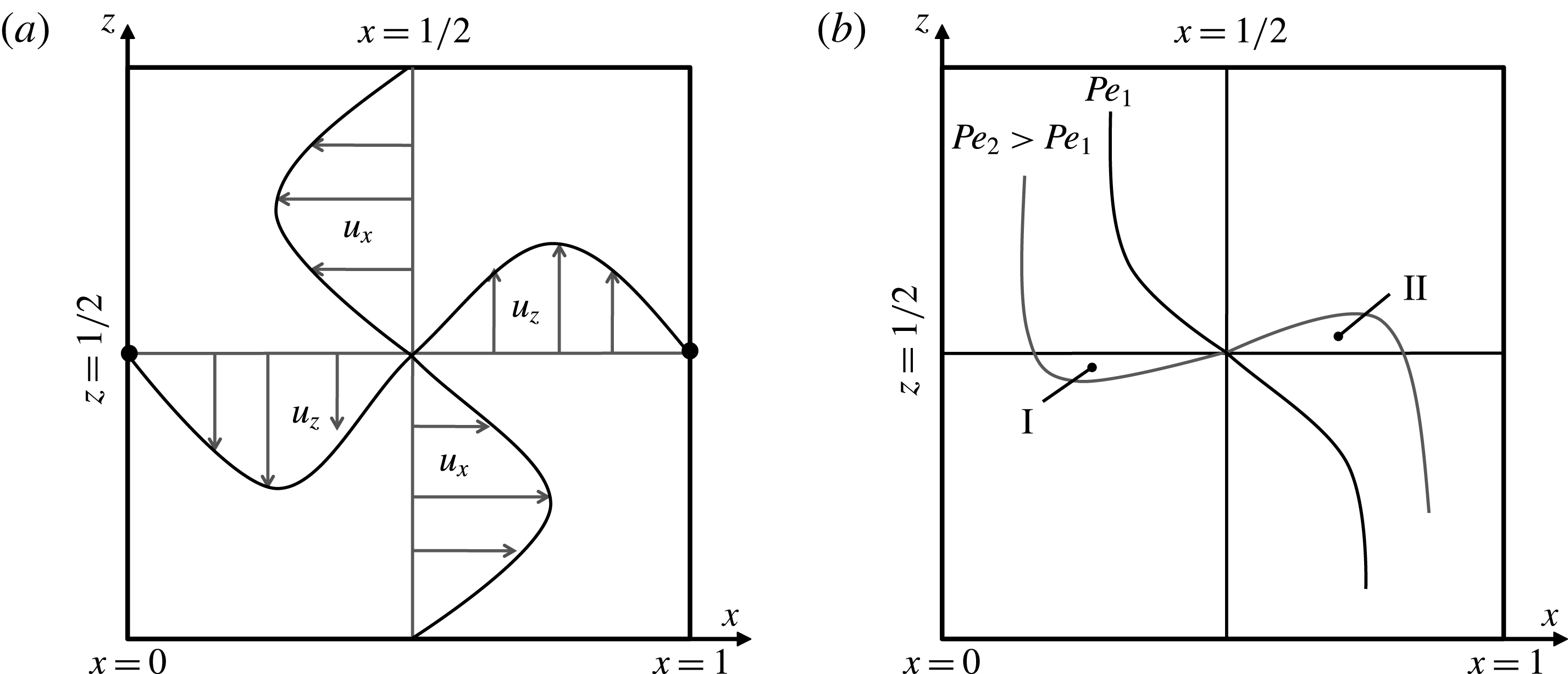
   where vanishing of $\unicode[STIX]{x1D706}_{1}$ and orientation of its eigenvector as $\boldsymbol{v}_{1}=\boldsymbol{e}_{y}$ reflect the fact that the stagnation point belongs to a stagnation line parallel to the $y$ -axis. Differential heating causes fluid to descend and rise at the cold ( $x=0$ ) and warm ( $x=1$ ) walls, respectively, inducing weak counter-clockwise rotation about $\boldsymbol{x}_{c}$ as shown schematically in figure 6(a). This gives rise to $\unicode[STIX]{x2202}u_{x}/\unicode[STIX]{x2202}z<0$ and $\unicode[STIX]{x2202}u_{z}/\unicode[STIX]{x2202}x>0$ and, inherently, $B_{0}<0$ , implying that $\boldsymbol{x}_{c}$ is a degenerate focus ( $A=0$ ), or equivalently, a centre. This is entirely consistent with the observations that $Gr=0$ yields a primary circulation consisting of concentric streamlines centred on one central stagnation line (see § 3).

2. (ii) ‘Small’  $Gr$ . This induces weak symmetry breaking, i.e. $\unicode[STIX]{x2202}u_{x}/\unicode[STIX]{x2202}x\sim O(\unicode[STIX]{x1D716})$ and $\unicode[STIX]{x2202}u_{z}/\unicode[STIX]{x2202}z\sim O(\unicode[STIX]{x1D716})$ , upon substitution in (4.2) yielding $B=B_{0}+O(\unicode[STIX]{x1D716}^{2})\approx B_{0}<0$ . Combined with $A=\unicode[STIX]{x2202}u_{x}/\unicode[STIX]{x2202}x+\unicode[STIX]{x2202}u_{z}/\unicode[STIX]{x2202}z\sim O(\unicode[STIX]{x1D716})$ this signifies the transition of the stagnation line into a focus-type stagnation point $\boldsymbol{x}_{c}$ with manifolds $W_{1D}={\mathcal{L}}$ and $W_{2D}={\mathcal{P}}$ (figure 5 a). Hence, the overall vortical structure associated with the primary circulation is preserved. The principal difference with the above limit $Gr=0$ exists in the formation of toroidal structures on both sides of ${\mathcal{P}}$ by the Hamiltonian mechanisms discussed in § 3.4.

Figure 6.

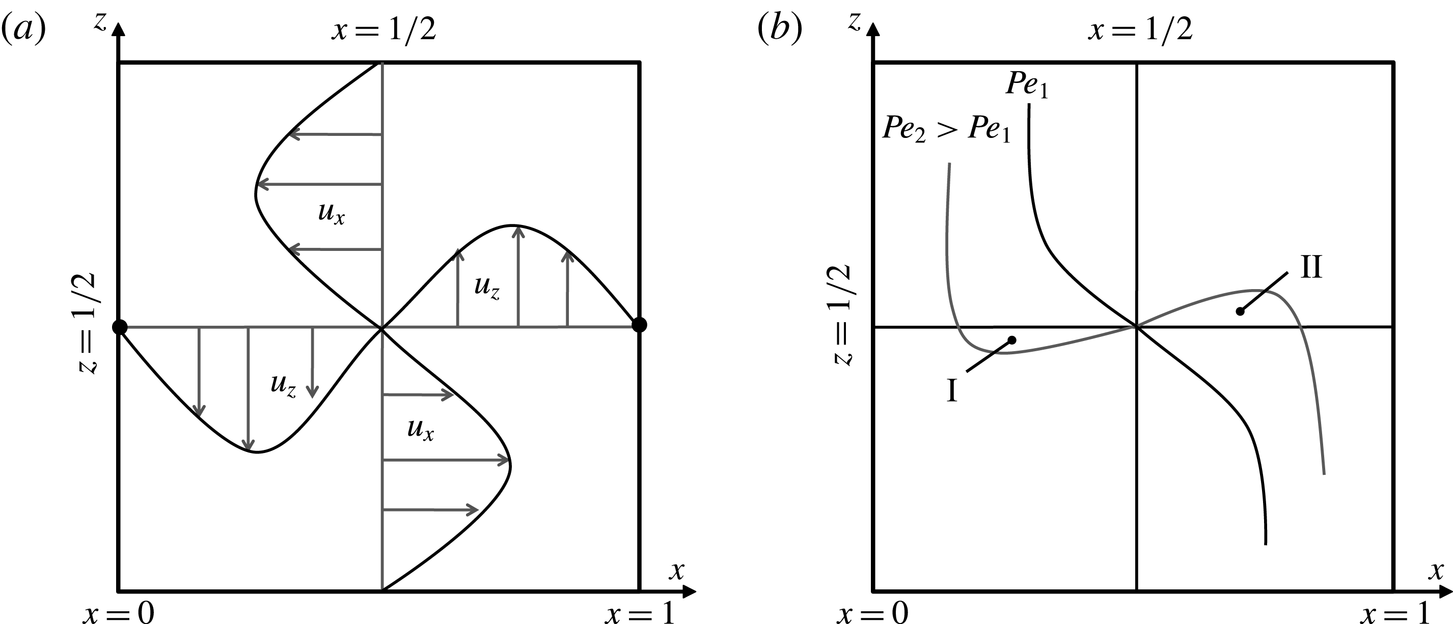
Thermal and flow phenomena underlying fundamental Lagrangian dynamics: (a) thermally induced counter-clockwise circulation about stagnation point $\boldsymbol{x}_{c}=(x,z)=(1/2,1/2)$ due to descent ( $u_{z}<0$ ) and ascent ( $u_{z}>0$ ) of fluid at the cold ( $x=0$ ) and warm ( $x=1$ ) walls, respectively; (b) flow-induced penetration of warm and cold temperature fronts in ‘cold’ ( $x<1/2$ ) and ‘warm’ regions ( $x>1/2$ ), respectively. The latter is illustrated with isotherm $T=1/2$ for ‘weaker’ ( $Pe_{1}$ ) and ‘stronger’ ( $Pe_{2}>Pe_{1}$ ) convective heat transfer (parameterised by Péclet number $Pe=GrPr$ ). For ‘sufficient’ $Pe$ (here $Pe=Pe_{2}$ ) this creates local heating (I) and cooling (II) zones adjacent to $\boldsymbol{x}_{c}$ .

The above demonstrates that progressively increasing $Gr$ from limit $Gr=0$ invariably induces a single focus-type stagnation point and, in consequence, a global circulation yielding a flow topology consisting of toroidal structures as illustrated above, advancing this as the universal ‘start-up’ scenario from said limit. Moreover, the topological equivalence with lid-driven flows established in § 3.3 puts forth fluid inertia as the dominant cause for symmetry breaking. This can be further substantiated by a leading-order approximation of the symmetry-breaking convective and buoyancy terms in (2.3) via decomposition of the flow and temperature fields as $\boldsymbol{u}=\boldsymbol{u}_{0}+\boldsymbol{u}^{\prime }$ and $\widehat{T}=\widehat{T}_{0}+\widehat{T}^{\prime }$ , where subscript ‘0’ and primes indicate the symmetric field for limit $Gr=0$ and associated small non-symmetric departure for ‘small’ $Gr>0$ , respectively. (Here $\widehat{T}$ corresponds with the redefined temperature according to § 3.2.) This gives

(4.4a,b ) $$\begin{eqnarray}\displaystyle -\!\unicode[STIX]{x1D735}\widehat{p}+\unicode[STIX]{x1D6FB}^{2}\boldsymbol{u}\approx Gr\boldsymbol{u}_{0}\boldsymbol{\cdot }\unicode[STIX]{x1D735}\boldsymbol{u}_{0}-\widehat{T}_{0}\boldsymbol{e}_{z},\quad \unicode[STIX]{x1D6FB}^{2}\widehat{T}=\unicode[STIX]{x1D6FB}^{2}\widehat{T}^{\prime }\approx GrPr\boldsymbol{u}_{0}\boldsymbol{\cdot }\unicode[STIX]{x1D735}\widehat{T}_{0}, & & \displaystyle\end{eqnarray}$$

revealing that the buoyancy term (to leading-order approximation) retains the symmetric form of limit $Gr=0$ on grounds of its linearity and, indeed, fluid inertia is the prevailing symmetry-breaking mechanism for the flow field in this first stage of $Gr>0$ . Convective heat transfer breaks the symmetry of the temperature field, yet here without appreciable ‘feedback’ into the momentum balance. This exposes the degree of asymmetry of the buoyancy term, determined by departure $\widehat{T}^{\prime }$ , yet not its presence and/or magnitude per se as cause behind thermally induced non-trivial Lagrangian dynamics. However, this asymmetry becomes significant only for ‘sufficiently large’ $Gr$ , as investigated in § 4.2.

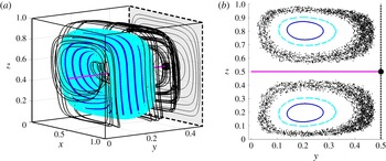
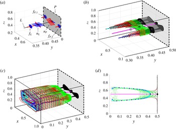
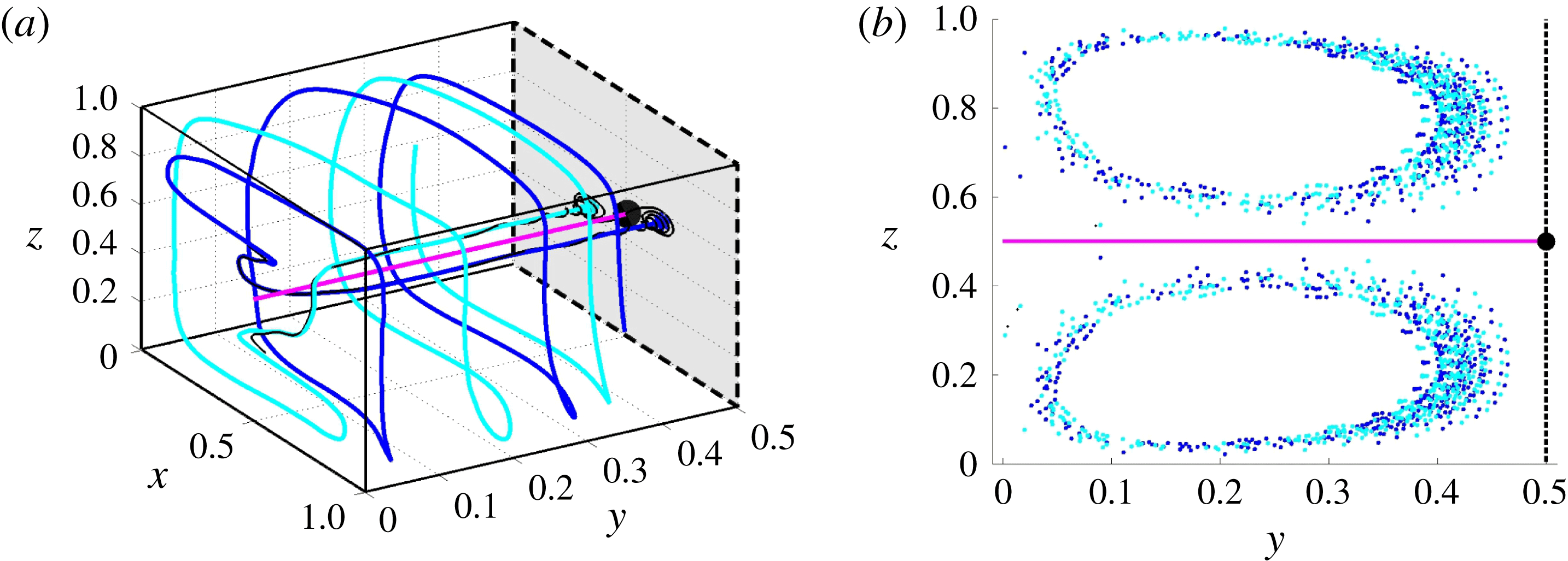
Figure 7(a) exemplifies the generic 3D flow topology in the inertia-dominated regime with case $Pr=0.71$ and $Gr=2.4\times 10^{4}$ . (The inertia-dominated case corresponds with the state denoted in the literature by, for example, ‘single-roll base flow’, ‘one-roll system’ or ‘one-roll convective cell’ (Mallinson & de Vahl Davis Reference Mallinson and de Vahl Davis1977; Hiller et al. Reference Hiller, Koch and Kowalewski1989; Yarin et al. Reference Yarin, Kowalewski, Hiller and Koch1996)) The key organising entities are the focus $\boldsymbol{x}_{c}$ (black marker), with ${\mathcal{P}}$ (dashed/shaded) and ${\mathcal{L}}$ (magenta) as associated 2D manifold $W_{2D}(\boldsymbol{x}_{c})$ and 1D manifold $W_{1D}(\boldsymbol{x}_{c})$ , respectively. The flow topology in each subregion separated by ${\mathcal{P}}$ consists of a single family of KAM tori (one specimen highlighted in blue) and island chains emanating from disintegrated tori (one specimen highlighted in cyan) centred on $W_{1D}(\boldsymbol{x}_{c})$ . These structures are typically surrounded by chaotic streamlines (one specimen indicated in black). Figure 7(b) gives the corresponding Poincaré section (plane $x=1/2$ ) of this generic topological composition. (The 3D view includes only a small part of the chaotic streamline for reasons of legibility.) Centrifugal forces cause outward spiralling away from $\boldsymbol{x}_{c}$ within ${\mathcal{P}}$ , implying repulsion in $W_{2D}(\boldsymbol{x}_{c})$ (i.e. $Re(\unicode[STIX]{x1D706}_{2,3})=A/2>0$ ) and, in consequence, attraction along $W_{1D}(\boldsymbol{x}_{c})$ (i.e. $\unicode[STIX]{x1D706}_{1}=-A=-2Re(\unicode[STIX]{x1D706}_{2,3})<0$ ). This renders the 1D and 2D manifolds stable ( $W_{1D}^{s}$ ) and unstable ( $W_{2D}^{u}$ ), respectively, in dynamical-systems terminology (Guckenheimer & Holmes Reference Guckenheimer and Holmes1983; Ott Reference Ott2002). The attraction along $W_{1D}^{s}$ drives the secondary circulation.

Figure 7.

Generic 3D flow topology in subregion $0\leqslant y\leqslant 1/2$ separated by ${\mathcal{P}}$ (dashed/shaded) in the inertia-dominated regime demonstrated for $Pr=0.71$ and $Gr=2.4\times 10^{4}$ : (a) 3D perspective view; (b) Poincaré section ( $x=1/2$ ). Key entities: focus $\boldsymbol{x}_{c}=(1/2,1/2,1/2)$ (black marker) with ${\mathcal{P}}$ and ${\mathcal{L}}$ (magenta) as associated 2D manifold and 1D manifold, respectively; KAM torus (blue); torus corresponding with island chains (cyan); 3D chaotic streamline (black).

Figure 8.

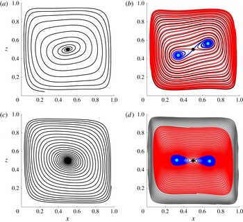
Typical streamline portraits in ${\mathcal{P}}$ before (a,c) and after (b,d) bifurcation of the central stagnation point (black marker) from focus to saddle (NSS in 3D) with accompanying pair of foci (cyan markers) demonstrated for $Pr=0.71$ (a,b) and $Pr=7$ (c,d): (a) pre-bifurcation ( $Gr=2.4\times 10^{4}$ ); (b) post-bifurcation ( $Gr=7.2\times 10^{4}$ ); (c) pre-bifurcation ( $Gr=1.3\times 10^{3}$ ); (d) post-bifurcation ( $Gr=1.0\times 10^{4}$ ). Blue streamline: stable manifold of saddle forming heteroclinic orbits with foci; red streamline: unstable manifold of saddle separating 2D manifolds of foci within the symmetry plane; black/grey curves: typical streamlines within each 2D manifold.

4.2 Second ‘stage’ of symmetry breaking: thermo-inertial flows

Convective heat transfer becomes stronger with increasing $Gr$ and thus, for ‘sufficient’ $Gr$ , causes symmetry breaking of the temperature field and, in consequence, of the buoyancy term to such an extent that it induces a global bifurcation in the flow topology, as demonstrated in figure 8 for the streamline portrait in ${\mathcal{P}}$ for $Pr=0.71$ (top) and $Pr=7$ (bottom). The stagnation point $\boldsymbol{x}_{c}$ (black marker) within ${\mathcal{P}}$ bifurcates from a focus for ‘smaller’ $Gr$ (panel a,c) to a saddle for ‘larger’ $Gr$ (panel b,d). Moreover, saddle-type $\boldsymbol{x}_{c}$ is accompanied by a pair of foci (cyan markers) arranged symmetrically according to centro-symmetry (3.2). The stable manifold of the saddle (blue streamline) forms heteroclinic orbits with the repelling foci; its unstable manifold (red streamline) separates the 2D manifolds of the foci within the symmetry plane (as demonstrated by typical streamlines in each 2D manifold indicated by the black/grey curves). This heteroclinic interaction gives rise to the ‘figure 8’ pattern emerging around $\boldsymbol{x}_{c}$ .

The general sense of circulation is retained upon bifurcation: fluid revolves in counter-clockwise direction around the pre-bifurcation focus as well as about the post-bifurcation individual foci (blue streamline) and the entire saddle–node arrangement (red streamline). Note that the bifurcated state is termed ‘two-roll system’ in Hiller et al. (Reference Hiller, Koch and Kowalewski1989), Yarin et al. (Reference Yarin, Kowalewski, Hiller and Koch1996); the vortical structures centred on the foci (blue) are denoted ‘secondary rolls’ in Mallinson & de Vahl Davis (Reference Mallinson and de Vahl Davis1977).

The above behaviour corresponds with a pitchfork bifurcation of the streamline pattern within ${\mathcal{P}}$ at stagnation point $\boldsymbol{x}_{c}$ (Ott Reference Ott2002). This is a direct consequence of two fundamental topological properties. First, centro-symmetry (3.2) causes stagnation points in the midplane other than $\boldsymbol{x}_{c}$ to emerge pair-wise following $(\boldsymbol{x}_{s},\boldsymbol{S}_{ii}(\boldsymbol{x}_{s}))$ . Second, the Poincaré-Hopf theorem states that the sum of the Poincaré indices $I_{i}$ of fixed (here stagnation) points equals the Euler characteristic $\unicode[STIX]{x1D712}$ of the invariant surface, i.e.

(4.5) $$\begin{eqnarray}\displaystyle \unicode[STIX]{x1D712}=\mathop{\sum }_{i=1}^{N}I_{i}, & & \displaystyle\end{eqnarray}$$

where $I=1$ and $I=-1$ for focus-type and saddle-type stagnation points, respectively (Henle Reference Henle1979). The Euler characteristic is a topological invariant for the invariant material plane ${\mathcal{P}}$ and, given ‘small’ $Gr$ always results in a single focus, here equals $\unicode[STIX]{x1D712}=1$ . Preservation of $\unicode[STIX]{x1D712}=1$ during bifurcation of $\boldsymbol{x}_{c}$ within ${\mathcal{P}}$ from focus to saddle thus dictates the emergence of a symmetric pair of focus-type stagnation points. (This again ignores the above-mentioned corner eddies and thus, strictly, pertains only to the subregion within ${\mathcal{P}}$ that excludes the corner regions. Moreover, this assumes that the separatrix between former and latter regions is unaffected by the bifurcation. However, given their localised and weak nature, the corner eddies changing due to the bifurcation and thereby simultaneously compromising the separatrix – and thus the reasoning in toto – is highly improbable.) The stagnation points in ${\mathcal{P}}$ may possibly undergo subsequent bifurcations upon further increasing $Gr$ . However, this is beyond the present scope.

The above focus-to-saddle transition corresponds in the 3D domain with a bifurcation of $\boldsymbol{x}_{c}$ from focus to NSS. The fact that topological constraints only admit saddle-type streamline portraits for $\boldsymbol{x}_{c}$ within ${\mathcal{P}}$ upon bifurcation has the fundamental implication that manifold $W_{2D}$ (accommodating node-type portraits) can not coincide with ${\mathcal{P}}$ and here, given $\boldsymbol{v}_{1}\in {\mathcal{L}}$ and $\boldsymbol{v}_{2,3}\in {\mathcal{P}}$ , thus must emerge from either the $(\boldsymbol{v}_{1},\boldsymbol{v}_{2})$ -plane or the $(\boldsymbol{v}_{1},\boldsymbol{v}_{3})$ -plane. Hence, strictly two configurations are permissible:

1. (i) $\text{sign}(\unicode[STIX]{x1D706}_{1})=\text{sign}(\unicode[STIX]{x1D706}_{3})=-\text{sign}(\unicode[STIX]{x1D706}_{2})\;\Rightarrow \;(\boldsymbol{v}_{1},\boldsymbol{v}_{3})\rightarrow W_{2D},\boldsymbol{v}_{2}\rightarrow W_{1D}$ ;

2. (ii) $\text{sign}(\unicode[STIX]{x1D706}_{1})=\text{sign}(\unicode[STIX]{x1D706}_{2})=-\text{sign}(\unicode[STIX]{x1D706}_{3})\;\Rightarrow \;(\boldsymbol{v}_{1},\boldsymbol{v}_{2})\rightarrow W_{2D},\boldsymbol{v}_{3}\rightarrow W_{1D}$ .

However, given that $\unicode[STIX]{x1D706}_{2,3}$ and associated eigenvectors $\boldsymbol{v}_{2,3}\in {\mathcal{P}}$ can be interchanged without loss of generality, both cases are in fact identical. Thus the former case, shown in figure 5(b–d), defines the generic configuration for NSS-type $\boldsymbol{x}_{c}$ , putting forth $W_{1D}\in {\mathcal{P}}$ and (near ${\mathcal{P}}$ ) $W_{2D}\bot {\mathcal{P}}$ as corresponding 3D manifold orientations (typical configurations are demonstrated in § 5.2.1). Moreover, $\text{sign}(\unicode[STIX]{x1D706}_{2})=-\text{sign}(\unicode[STIX]{x1D706}_{3})$ via (4.2) gives inequality $\unicode[STIX]{x1D706}_{2}\unicode[STIX]{x1D706}_{3}=A^{2}/4-B\leqslant 0$ . Hence, $B=0$ implies $A=0$ , meaning that the pitchfork bifurcation always happens through the degenerate case $\unicode[STIX]{x1D706}_{1}=\unicode[STIX]{x1D706}_{2}=\unicode[STIX]{x1D706}_{3}=0$ .

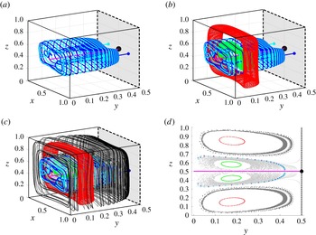
Figure 9(a) gives the Poincaré section ( $x=1/2$ ) corresponding with $(Pr,Gr)=(7,1.0\times 10^{4})$ as shown in figure 8(d), exposing a secondary family of KAM tori around the symmetry line ${\mathcal{L}}$ at the cavity wall $y=0$ , accommodating secondary circulation in the reversed direction of the original (‘primary’) family of tori (i.e. counter-clockwise and clockwise secondary circulation for primary and secondary tori, respectively). Such secondary tori have, to the best of our knowledge, not been explicitly reported before. (The two tori families are reminiscent of the two kinds of spiralling streamlines, distinguished by ‘forward’ and ‘reversed’ flow, in the post-bifurcation case in Mallinson & de Vahl Davis (Reference Mallinson and de Vahl Davis1977). However, the fact that the latter (i) include (one of) the secondary roll(s) and (ii) involve secondary circulation in directions opposite to that of the above tori strongly suggests that these are essentially different entities. The ‘forward-flow’ streamlines adjacent to the $y$ -wise endwalls likely result from the $y$ -wise elongated cavity (height : width  = 1 : 2) and therefore have no counterpart in the current cubic cavity. Moreover, comparison with findings in § 5.2 suggests that the ‘reversed-flow’ streamlines adjacent to symmetry plane ${\mathcal{P}}$ belong to the chaotic region in between primary and secondary tori.) The spatial extent of these new entities expands (while maintaining circulation direction) with increasing $Gr$ , as demonstrated in figure 9(b,c) for $Gr=1.7\times 10^{4}$ and $Gr=2.5\times 10^{4}$ , respectively, at $Pr=7$ . Moreover, their emergence is a consequence of intricate 3D heteroclinic interactions between the manifolds of the above-mentioned stagnation points in ${\mathcal{P}}$ and new stagnation points on ${\mathcal{L}}$ . This is further studied in § 5.

Figure 9.

Emergence of secondary family of KAM tori around ${\mathcal{L}}$ (dashed) at cavity wall $y=0$ and its expansion with growing $Gr$ demonstrated for $Pr=7$ : (a) $Gr=1.0\times 10^{4}$ ;(b) $Gr=1.7\times 10^{4}$ ; (c) $Gr=2.5\times 10^{4}$ . Visualisation by the left half ( $0\leqslant y\leqslant 1/2$ ) of Poincaré sections ( $x=1/2$ ).

The pitchfork bifurcation has been observed in numerous studies in both 2D and 3D systems, see, for example, de Vahl Davis (Reference de Vahl Davis1968), Mallinson & de Vahl Davis (Reference Mallinson and de Vahl Davis1973), Mallinson & de Vahl Davis (Reference Mallinson and de Vahl Davis1977), de Vahl Davis (Reference de Vahl Davis1983), Markatos & Pericleous (Reference Markatos and Pericleous1984), Hiller et al. (Reference Hiller, Koch and Kowalewski1989), Hiller et al. (Reference Hiller, Koch, Kowalewski, de Vahl Davis, Behnia, Moffatt and Tsinober1990), Yarin et al. (Reference Yarin, Kowalewski, Hiller and Koch1996), and occurs in a similar way for basically any $Pr$ . The impact of the latter is mainly quantitative in that secondary circulation becomes weaker with increasing $Pr$ , and streamlines, in consequence, tend towards denser winding; compare to this end, for example, figure 8(b,d) and refer, for example, also to Mallinson & de Vahl Davis (Reference Mallinson and de Vahl Davis1977).

4.3 Bifurcation mechanism

The pitchfork bifurcation for ‘sufficiently large’ $Gr$ admits physical explanation by continuing the examination of the properties of the stagnation point $\boldsymbol{x}_{c}$ in § 4.1. Transition of $\boldsymbol{x}_{c}$ from a focus into a NSS happens for parameter $B\geqslant 0$ in (4.2) and thus advances

(4.6) $$\begin{eqnarray}\displaystyle B\geqslant 0\quad \Rightarrow \quad B_{0}\geqslant B_{0}^{\ast }\quad \text{with }B_{0}^{\ast }=-\frac{1}{4}\left[\frac{\unicode[STIX]{x2202}u_{x}}{\unicode[STIX]{x2202}x}-\frac{\unicode[STIX]{x2202}u_{z}}{\unicode[STIX]{x2202}z}\right]^{2}<0, & & \displaystyle\end{eqnarray}$$

as the kinematic bifurcation criterion. For (generically) non-zero $\unicode[STIX]{x2202}u_{x,z}/\unicode[STIX]{x2202}x,z$ this sets a negative lower bound for $B_{0}$ (as opposed to $B_{0}\geqslant 0$ above), meaning that the flow admits the bifurcation for a circulation in the sense shown in figure 6(a). Hence, this is indeed the first (in a possible sequence of) bifurcation(s) undergone by the streamline pattern set up at $Gr=0$ . Physical considerations suggest that stronger convective heat transfer (by increasing Péclet number $Pe=GrPr$ through, for given $Pr$ , increasing $Gr$ ) promotes exceeding threshold (4.6) and, inherently, the bifurcation. Stronger convective heat transfer namely admits deeper penetration of the warm and cold temperature fronts in the ‘cold’ ( $x<1/2$ ) and ‘warm’ regions ( $x>1/2$ ), respectively, in a manner as illustrated in figure 6(b) with isotherm $T=1/2$ . (Symmetry dictates this isotherm to remain attached to the stagnation point $\boldsymbol{x}_{c}$ and satisfy centro-symmetry (3.2) for any $Gr$ and $Pr$ .) The latter (and any other isotherm) emanates from ‘coiling up’ of the vertical isotherms of limit $Gr=0$ shown in figure 2(a) due to the circulation about the cavity centre for $Gr>0$ . The convolution becomes more pronounced with increasing $Pe=GrPr$ , and thus causes ever deeper penetration of said temperature fronts. For $Pe=GrPr$ beyond a certain threshold ( $Pe_{2}$ in figure 6 b) this results in formation of local heating (I) and cooling (II) zones adjacent to $\boldsymbol{x}_{c}$ . This locally reduces buoyancy and, in consequence, flattens the $u_{z}$ -profile (and, via continuity, also the $u_{x}$ -profile), thus effectively shifting $B_{0}<B_{0}^{\ast }<0$ towards threshold $B_{0}=B_{0}^{\ast }$ following (4.6). The bifurcation occurs when the shift suffices to cross this threshold, or equivalently, an associated threshold $Gr^{\ast }$ .

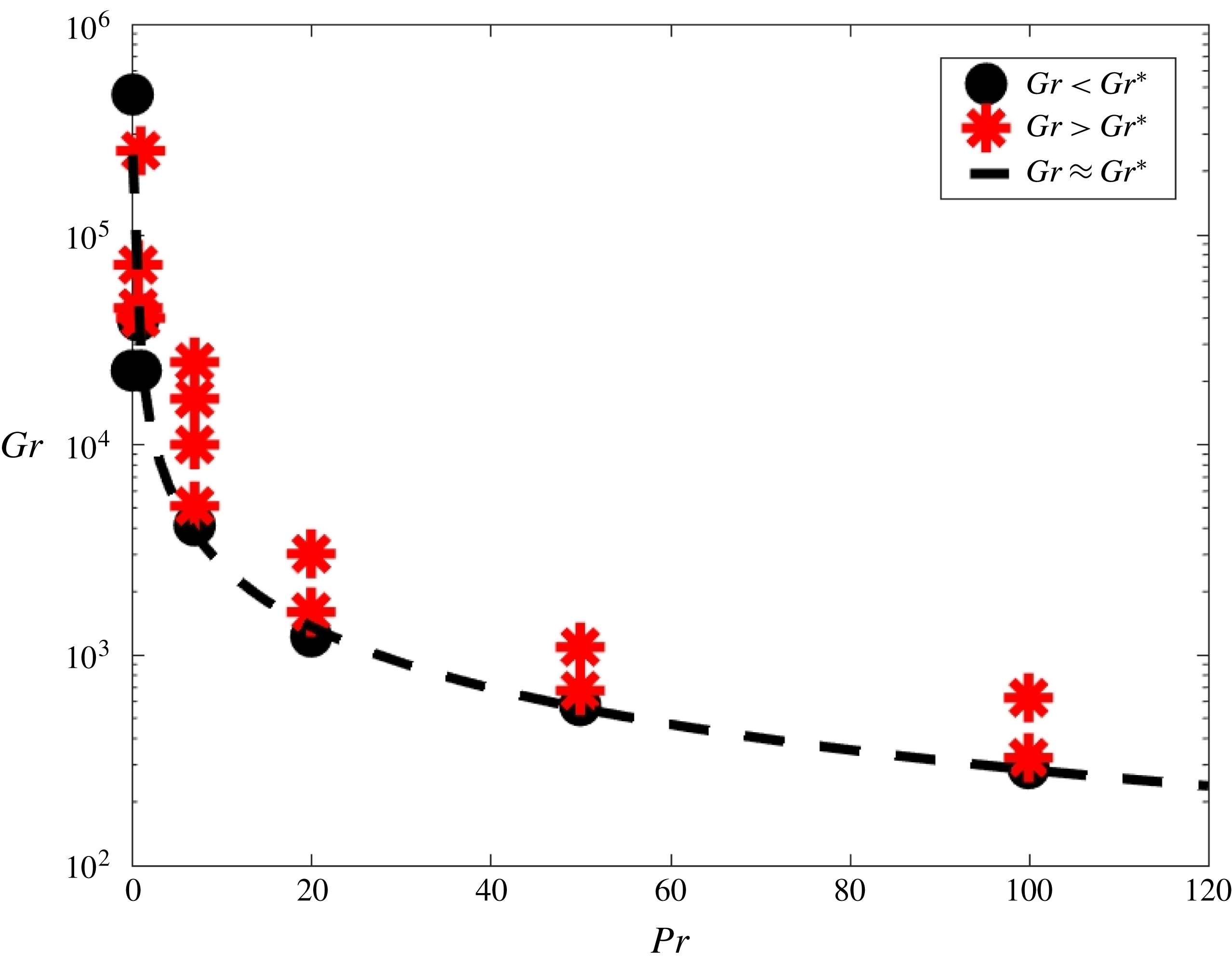
The pitchfork bifurcation happens at any $Pr$ upon exceeding $Gr=Gr^{\ast }$ , as confirmed by the corresponding bifurcation diagram in figure 10. Moreover, this reveals, consistent with figure 8, a decreasing threshold $Gr^{\ast }$ , and thus earlier bifurcation, with growing $Pr$ . This stems from the existence of two limits of the governing equations (2.3) in $Pr$ . Limit $Pr=0$ : symmetry breaking solely by fluid inertia due to the absence of convective heat transfer; limit $Pr\rightarrow \infty$ : symmetry breaking dominated by buoyancy via strongly asymmetric temperature fields due to purely convective heat transfer. The former and latter imply absence and immediate onset, respectively, of the pitchfork bifurcation on the route starting from limit $Gr=0$ and define asymptotes for the bifurcation threshold following

(4.7a,b ) $$\begin{eqnarray}\displaystyle \lim _{Pr\rightarrow 0}Gr^{\ast }\rightarrow \infty ,\quad \lim _{Pr\rightarrow \infty }Gr^{\ast }=0, & & \displaystyle\end{eqnarray}$$

which qualitatively ‘shape’ the bifurcation diagram. (Temperature becomes a passive tracer for unbounded $Pr$ , i.e. $\lim _{Pr\rightarrow \infty }\text{d}T/\text{d}t=\boldsymbol{u}\boldsymbol{\cdot }\unicode[STIX]{x1D735}T=0$ , causing direct transport of temperature fronts with material fluid interfaces via the incipient circulation sketched in figure 6(a), and thus their immediate penetration according to figure 6(b).) The threshold monotonically decreases with growing $Pr$ during the transition from inertia-dominated (‘small’ $Pr$ ) to buoyancy-dominated (‘large’ $Pr$ ) symmetry breaking. Asymptotes (4.7) suggest a hyperbolic relation $Gr^{\ast }=aPr^{b}$ ; the dashed curve in figure 10 gives this relation using coefficients $(a,b)=(2.53\times 10^{4},-0.97)$ determined via the least-squares method.

Figure 10.

Bifurcation diagram for the pitchfork bifurcation: threshold $Gr^{\ast }$ versus $Pr$ . Symbols indicate data points from numerical simulations; the dashed curve indicates the approximate bifurcation threshold $Gr\approx aPr^{b}$ , with coefficients $(a,\!b)=(2.53\times 10^{4},-0.97)$ .

The above designates buoyancy as the mechanism that underlies the pitchfork bifurcation, and $Gr$ as its key control parameter, and thus rigorously supports phenomenological explanations in the literature (as, for example, in de Vahl Davis (Reference de Vahl Davis1968), Mallinson & de Vahl Davis (Reference Mallinson and de Vahl Davis1977)). It furthermore substantiates the earlier finding in § 4.1 that, irrespective of $Pr$ , the formation of a single global vortical structure as illustrated in figure 7 is the only possible ‘start-up’ scenario of the flow upon increasing $Gr$ from zero. Hence, the bifurcation into a more complex vortical structure must (for realistic $Pr$ ) happen at some finite $Gr$ , and thus is an essentially nonlinear phenomenon.

The bifurcated streamline pattern is reminiscent of that occurring in lid-driven cavity flows with simultaneous forcing by facing walls moving steadily at the same speed in opposite direction (Kelmanson & Lonsdale Reference Kelmanson and Lonsdale1996; Shankar Reference Shankar1998). This extends the link with lid-driven cavity flows established in § 3. However, important to note is that this second connection exists only for the post-bifurcation case, in other words, for $Gr$ above some finite lower bound. A linear limit $Gr=0$ topologically equivalent to two-wall lid-driven flows is non-existent.

5.1 General behaviour associated with the pitchfork bifurcation

The streamline patterns corresponding with the cases in the bifurcation diagram, and comparison with the literature (Mallinson & de Vahl Davis Reference Mallinson and de Vahl Davis1977; Yarin et al. Reference Yarin, Kowalewski, Hiller and Koch1996), strongly suggests that, overall, the bifurcated 3D flow topologies are qualitatively similar (at least) up to $Pr\sim O(6\times 10^{3})$ . Two fundamentally different situations can be distinguished in this range: cases with and without secondary tori. The bifurcated 3D topologies of cases $Pr=7$ and $Pr=0.71$ in figure 8, for example, correspond to former and latter situations, respectively. Secondary tori are separated from the primary tori by a ‘separatrix’ formed by intricate 3D heteroclinic manifold interactions of stagnation points on ${\mathcal{P}}$ and ${\mathcal{L}}$ (elaborated in § 5.2) and are for the cases included in the bifurcation diagram found only for $Pr\geqslant 7$ ; they are absent for all ‘smaller’ $Pr$ (here $Pr\leqslant 1$ ). This suggests that secondary tori emerge only for ‘larger’ $Pr$ due to topological bifurcation(s) within regime $Gr\geqslant Gr^{\ast }$ corresponding with the Prandtl number $Pr$ . Given the transition from inertia-dominated to buoyancy-dominated dynamics with increasing $Pr$ (§ 4.3), this designates secondary tori as a buoyancy-induced phenomenon that occurs upon exceeding a certain threshold $Pr^{\ast }$ . (Thus dividing regime $Gr>Gr^{\ast }$ in the bifurcation diagram in figure 10 into subregimes $Pr\leqslant Pr^{\ast }$ and $Pr>Pr^{\ast }$ .) Moreover, secondary tori always appear at the cavity endwalls and gradually expand towards ${\mathcal{P}}$ with increasing $Gr$ in a similar way as demonstrated in figure 9 for $Pr=7$ . Hence, the bifurcated flow topology at $Pr=7$ is typical of that for ‘larger’ $Pr$ (i.e. $Pr>Pr^{\ast }$ ) in general. Note for reference that Prandtl numbers of realistic fluids span many orders of magnitude, ranging from $Pr\sim O(10^{-2})$ for liquid metals via $Pr\sim O(1)$ and $Pr\sim O(10)$ for air and water, respectively, to $Pr\sim O(10^{4}-10^{8})$ for magma (Lappa Reference Lappa2010).

Furthermore, the saddle-foci arrangement may undergo stability reversal upon further increasing $Gr$ : foci become attracting within ${\mathcal{P}}$ and form a heteroclinic orbit with the unstable manifold of the saddle. Concurrently with stability reversal, a closed streamline emerges within ${\mathcal{P}}$ that encloses the saddle-foci arrangement and acts as a repelling limit cycle for the stable manifold of the saddle. The flow topology inside the area enclosed by the limit cycle nonetheless remains as in figure 8(b,d), yet with now the unstable and stable manifold of the saddle coiling up around the foci and spiralling outward, respectively, in counter-clockwise direction (thus maintaining the sense of the primary circulation). Such stability reversal, for example, happens for $Pr=7$ between $Gr=1.7\times 10^{4}$ (original stability) and $Gr=2.5\times 10^{4}$ (reversed stability). However, the impact on the flow topology is marginal and localised in that certain heteroclinic interactions between the several stagnation points may change yet without essentially affecting the overall structure and role of the above-mentioned separatrix. The global partitioning into two families of KAM tori (and the corresponding sense of circulation) is retained, as evidenced by the (qualitatively) identical composition of the Poincaré sections for $Gr=1.0\times 10^{4},1.7\times 10^{4}$ (original stability) and $2.5\times 10^{4}$ (reversed stability) in figure 9. Hence, stability reversal, given its secondary role in the global 3D Lagrangian dynamics, is not examined further here.

Typical bifurcated 3D flow topologies with and without secondary tori are demonstrated below in §§ 5.2 and 5.3, respectively. First insights into the mechanisms underlying their 3D structure and organisation are obtained through analysis of heteroclinic interactions between the several stagnation points.

5.2 Presence of secondary tori (fluids with ‘larger’ $Pr$ )

5.2.1 Stagnation points and associated manifolds

Figure 11.

Typical configuration of stagnation points in symmetry plane/line ( ${\mathcal{P}}/{\mathcal{L}}$ ) and associated manifolds in bifurcated 3D flow topology demonstrated for $Pr=7$ and $Gr=2.5\times 10^{4}$ : (a) stagnation points $(\boldsymbol{f}_{{\mathcal{P}},1,2},\boldsymbol{n}_{{\mathcal{P}}},\boldsymbol{f}_{{\mathcal{L}}},\boldsymbol{n}_{{\mathcal{L}}})$ (black stars) and local orientation of associated 1D (lines) and 2D (planes/disks) manifolds (blue/red: stable/unstable); (b) 3D manifold configuration encompassing $W_{1D}^{u}(\boldsymbol{f}_{{\mathcal{P}},1,2})$ (blue/cyan), $W_{2D}^{u}(\boldsymbol{n}_{{\mathcal{P}}})$ (grey/black), $W_{1D}^{u}(\boldsymbol{n}_{{\mathcal{L}}})$ (red), $W_{2D}^{s}(\boldsymbol{n}_{{\mathcal{L}}})$ (green) and heteroclinic orbit ${\mathcal{L}}=(W_{2D}^{u}(\boldsymbol{n}_{{\mathcal{P}}})\cap W_{2D}^{s}(\boldsymbol{n}_{{\mathcal{L}}}))\cup W_{1D}^{s}(\boldsymbol{f}_{{\mathcal{L}}})$ (magenta); (c) global foliation of manifolds ( $W_{2D}$ represented by single constituent streamline); (d) Poincaré section $x=1/2$ (shows larger portions of streamlines than in panel c). Note that $W_{2D}^{u}$ of $\boldsymbol{f}_{{\mathcal{L}}}$ (grey marker in panels b–d) is not included due to its localised nature.

Case $Pr=7$ and $Gr=2.5\times 10^{4}$ is adopted hereafter as a typical bifurcated 3D flow topology with secondary tori as occurring for ‘larger’ $Pr$ (i.e. $Pr>Pr^{\ast }$ ). The stagnation points here consist of the above-mentioned NSS $(\boldsymbol{n}_{{\mathcal{P}}})$ and pair of foci ( $\boldsymbol{f}_{{\mathcal{P}},1}$ and $\boldsymbol{f}_{{\mathcal{P}},2}$ ) within ${\mathcal{P}}$ and a single NSS $(\boldsymbol{n}_{{\mathcal{L}}})$ and focus $(\boldsymbol{f}_{{\mathcal{L}}})$ on ${\mathcal{L}}$ . (Note that all non-degenerate stagnation points in incompressible flows are either NSS or focus; Chong et al. (Reference Chong, Perry and Cantwell1990).) Figure 11(a) gives the position of the stagnation points (black stars) including the local orientation of the associated 1D/2D manifold pairs (extent exaggerated for visibility) spanned by the corresponding eigenvectors $\boldsymbol{v}$ of the strain-rate tensor $\unicode[STIX]{x1D641}$ . 1D manifolds ( $W_{1D}$ ) are indicated by lines; 2D manifolds ( $W_{2D}$ ) are indicated by planes and disks for NSSs and foci, respectively. Blue/red objects represent stable ( $W^{s}$ ) and unstable ( $W^{u}$ ) manifolds; heavy lines and spirals within 2D manifolds indicate principal axes and typical trajectory for NSSs and foci, respectively. Note that the eigenvector(s) spanning a certain 1D/2D manifold are on grounds of symmetry either parallel or normal to ${\mathcal{P}}$ . The specific manifold configurations are $(W_{1D}^{s},W_{2D}^{u})$ for $\boldsymbol{n}_{{\mathcal{P}}}$ (oriented as $W_{1D}\in {\mathcal{P}}$ and $W_{2D}\bot {\mathcal{P}}$ following § 4.2) and $(W_{1D}^{u},W_{2D}^{s})$ for all other stagnation points.

The general 3D manifold structure and configuration are demonstrated in figure 11(b). Manifolds $W_{1D}^{u}(\boldsymbol{f}_{{\mathcal{P}},1,2})$ (blue/cyan streamlines) emerge perpendicularly from ${\mathcal{P}}$ and initially run parallel to ${\mathcal{L}}$ (magenta). Note that a first schematic of $W_{1D}^{u}(\boldsymbol{f}_{{\mathcal{P}},1,2})$ is provided in Hiller et al. (Reference Hiller, Koch and Kowalewski1989). Line ${\mathcal{L}}$ , in turn, constitutes the heteroclinic orbits between $\boldsymbol{n}_{{\mathcal{P}}}$ (black sphere), $\boldsymbol{n}_{{\mathcal{L}}}$ (black star) and $\boldsymbol{f}_{{\mathcal{L}}}$ (grey star). Manifold $W_{2D}^{u}(\boldsymbol{n}_{{\mathcal{P}}})$ , part of which is delineated by the grey stream surface bounded by heavy black streamlines, emanates in two directions from ${\mathcal{L}}$ and subsequently coils up on each side around $W_{1D}^{u}(\boldsymbol{f}_{{\mathcal{P}},1})$ and $W_{1D}^{u}(\boldsymbol{f}_{{\mathcal{P}},2})$ while gradually ‘spiralling away’ from ${\mathcal{P}}$ . This underlies the secondary rolls reported in Mallinson & de Vahl Davis (Reference Mallinson and de Vahl Davis1977). (Here the final segment of the shown part of $W_{2D}^{u}(\boldsymbol{n}_{{\mathcal{P}}})$ is visualised only by the bounding streamline starting closest to ${\mathcal{P}}$ .) Manifold $W_{2D}^{s}(\boldsymbol{f}_{{\mathcal{L}}})$ (grey star) is highly localised due to rapid disintegration already at small distances from ${\mathcal{L}}$ . Hence, this entity is not included in figure 11 for reasons of legibility and, given its minor role, omitted in the remaining discussion.

Manifold $W_{1D}^{u}(\boldsymbol{n}_{{\mathcal{L}}})$ (red streamline) shadows individual streamlines within $W_{2D}^{u}(\boldsymbol{n}_{{\mathcal{P}}})$ by coiling up around $W_{1D}^{u}(\boldsymbol{f}_{{\mathcal{P}},1,2})$ while spiralling away from ${\mathcal{P}}$ in essentially the same way. Manifold $W_{2D}^{s}(\boldsymbol{n}_{{\mathcal{L}}})$ is partially delineated by the green stream surface (bounded by thin black streamlines) and emanates in two directions from ${\mathcal{L}}$ in a manner resembling $W_{2D}^{u}(\boldsymbol{n}_{{\mathcal{P}}})$ . However, an essential difference between both entities is that $W_{2D}^{s}(\boldsymbol{n}_{{\mathcal{L}}})$ , instead of coiling up individually around $W_{1D}^{u}(\boldsymbol{f}_{{\mathcal{P}},1})$ and $W_{1D}^{u}(\boldsymbol{f}_{{\mathcal{P}},2})$ , layers itself around the entire structure defined by $W_{2D}^{u}(\boldsymbol{n}_{{\mathcal{P}}})$ and $W_{1D}^{u}(\boldsymbol{n}_{{\mathcal{L}}})$ .

Figure 11(b) exposes the central role of manifolds $W_{1D}^{u}$ of foci $\boldsymbol{f}_{{\mathcal{P}},1,2}$ in the global 3D flow topology by ‘arranging’ all other manifolds. The latter continue to closely follow manifolds $W_{1D}^{u}(\boldsymbol{f}_{{\mathcal{P}},1,2})$ while foliating throughout the entire 3D domain, as demonstrated in figure 11(c,d), which further substantiates this central role. (Here $W_{2D}^{u}(\boldsymbol{n}_{{\mathcal{P}}})$ and $W_{2D}^{s}(\boldsymbol{n}_{{\mathcal{L}}})$ are each represented by way of a single constituent streamline.) Moreover, this reveals that manifolds $W_{1D}^{u}(\boldsymbol{f}_{{\mathcal{P}},1,2})$ set up a secondary circulation normal to ${\mathcal{P}}$ akin to the inertia-dominated regime, which is particularly visible in the corresponding Poincaré section in figure 11(d). Note that the latter corresponds with larger portions of the streamlines than shown in figure 11(c). Comparison of figure 11(d) with figure 9(c) reveals that manifolds $W_{1D}^{u}(\boldsymbol{f}_{{\mathcal{P}},1,2})$ outline the above-mentioned separatrix between the primary and secondary KAM tori. This is elaborated in § 5.2.2.

The Poincaré section of $W_{2D}^{s}(\boldsymbol{n}_{{\mathcal{L}}})$ (green markers) clearly signifies chaotic behaviour that, given being interspersed with the Poincaré sections of $W_{2D}^{u}(\boldsymbol{n}_{{\mathcal{P}}})$ (black markers), $W_{1D}^{u}(\boldsymbol{n}_{{\mathcal{L}}})$ (red markers) and $W_{1D}^{u}(\boldsymbol{f}_{{\mathcal{P}},1,2})$ (blue/cyan markers), ensues from heteroclinic intersections $W_{2D}^{s}(\boldsymbol{n}_{{\mathcal{L}}})\cap W_{2D}^{u}(\boldsymbol{n}_{{\mathcal{P}}})$ and $W_{1D}^{u}(\boldsymbol{f}_{{\mathcal{P}},1,2})\cap W_{2D}^{s}(\boldsymbol{n}_{{\mathcal{L}}})$ and homoclinic intersections $W_{2D}^{s}(\boldsymbol{n}_{{\mathcal{L}}})\cap W_{1D}^{u}(\boldsymbol{n}_{{\mathcal{L}}})$ . Intersections between these manifolds (and possibly those of further undetected stagnation points) namely are signatures of chaotic dynamics (Ott Reference Ott2002; Meiss Reference Meiss2015). Note that $W_{1D}^{u}(\boldsymbol{n}_{{\mathcal{L}}})$ and $W_{2D}^{u}(\boldsymbol{n}_{{\mathcal{P}}})$ cannot intersect on grounds of equal stability properties. Moreover, restriction of $W_{1D}^{s}(\boldsymbol{n}_{{\mathcal{P}}})$ to ${\mathcal{P}}$ due to reflectional symmetry (3.1) excludes this entity from involvement in the 3D chaotic dynamics.

5.2.2 Arrangement of coherent structures

Figure 12.

Typical bifurcated 3D flow topology in subregion $0\leqslant y\leqslant 1/2$ separated by ${\mathcal{P}}$ (dashed/shaded) demonstrated for $Pr=7$ and $Gr=2.5\times 10^{4}$ :(a) formation of ‘skeleton’ by $W_{1D}^{u}(\boldsymbol{f}_{{\mathcal{P}},1,2})$ (blue/cyan) centred on ${\mathcal{L}}$ (magenta) partitioning shown subregion into interior and exterior zones; (b) interior (green) and exterior (red) families of KAM tori separated by ‘skeleton’; (c) interior (light grey) and exterior (dark grey/black) chaotic streamlines; (d) Poincaré section $x=1/2$ (shows larger portion of chaotic streamlines than in panel c.)

The 1D manifolds $W_{1D}^{u}$ of foci $\boldsymbol{f}_{{\mathcal{P}},1,2}$ tend to converge on NSS $\boldsymbol{n}_{{\mathcal{L}}}$ , which must be attributed to the heteroclinic intersections $W_{1D}^{u}(\boldsymbol{f}_{{\mathcal{P}},1,2})\cap W_{2D}^{s}(\boldsymbol{n}_{{\mathcal{L}}})$ , and thus describe a cocoon-like ‘skeleton’ that forms the ‘backbone’ of a chaotic region. This structure is clearly outlined by the blue/cyan markers and curves in figures 11(d) and 12(a), respectively, and partitions the subregion on each side of ${\mathcal{P}}$ into a zone interior and exterior to the skeleton. Thus the skeleton constitutes the above-mentioned separatrix between primary (exterior zone) and secondary (interior zone) tori. The skeleton consisting of streamlines, i.e. $W_{1D}^{u}(\boldsymbol{f}_{{\mathcal{P}},1,2})$ , means that the partitioning is not strict; transport across this entity is possible yet severely impeded. Hence, the skeleton defines a porous transport barrier reminiscent of cantori (MacKay, Meiss & Percival Reference MacKay, Meiss and Percival1984) and typically restricts tracers to one zone for prolonged periods of time. This is demonstrated in figure 11(d) by the Poincaré sections of streamlines belonging to $W_{2D}^{u}(\boldsymbol{n}_{{\mathcal{P}}})$ (black markers) and $W_{1D}^{u}(\boldsymbol{n}_{{\mathcal{L}}})$ (red markers). Both streamlines remain trapped in the skeleton proximity for a substantial time, yet eventually ‘escape’ near ${\mathcal{P}}$ (dashed line) into the exterior zone. (Note that the ‘reversed-flow’ streamlines adjacent to symmetry plane ${\mathcal{P}}$ in Mallinson & de Vahl Davis (Reference Mallinson and de Vahl Davis1977) closely resemble $W_{1D}^{u}(\boldsymbol{f}_{{\mathcal{P}},1,2})$ , lending credence to the earlier remark in § 4.2 that they likely belong to the above-mentioned chaotic region.)

The skeleton region originates from intricate manifold interactions corresponding with isolated stagnation points and, given the Hamiltonian structure of the Lagrangian equations of motion (§ 3.4) breaks down near such points (Bajer Reference Bajer1994), accommodates essentially 3D non-Hamiltonian dynamics. The Lagrangian behaviour within the zones interior and exterior to the skeleton, on the other hand, retains its Hamiltonian nature and thus is essentially similar to that in the inertia-dominated regime shown in figure 7. The flow topology in each zone namely consists of a single family of KAM tori centred on ${\mathcal{L}}$ , viz. said primary (exterior) and secondary (interior) tori, of which one specimen is highlighted in green and red, respectively, in figure 12(b), and island chains (not shown). These coherent structures, in turn, are surrounded by chaotic streamlines, with one interior and two exterior specimens indicated in light grey and black/dark grey, respectively, in figure 12(c). The corresponding Poincaré section is given in figure 12(d) and exposes the full topological make-up. (The 3D perspective shows only part of the chaotic streamlines for reasons of legibility.) The interior chaotic streamline further demonstrates the nature and impact of the skeleton on the Lagrangian dynamics by remaining confined to this zone for a prolonged period of time before eventually ‘escaping’ into the chaotic region of the exterior zone. Note that the relatively denser winding of the exterior chaotic streamlines indicates a lower intensity in chaotic dynamics compared to the interior zone.

Figure 13.

Bifurcated 3D flow topology in subregion $0\leqslant y\leqslant 1/2$ separated by ${\mathcal{P}}$ (dashed/shaded) for $Pr=0.71$ and $Gr=7.2\times 10^{4}$ : (a) formation of ‘skeleton’ by $W_{1D}^{s}(\boldsymbol{f}_{{\mathcal{P}},1,2})$ (blue/cyan) centred on ${\mathcal{L}}$ (magenta) and encircled by a single streamline within $W_{2D}^{s}(\boldsymbol{n}_{{\mathcal{P}}})$ (black); (b) Poincaré section $x=1/2$ (shows larger portion of streamlines than in panel a.)

Examination of the post-bifurcation topologies for $Pr=(20,50,100)$ reveals essentially the same behaviour as above for $Pr=7$ . Secondary tori appear near bounding wall $y=0$ and gradually expand towards symmetry plane ${\mathcal{P}}$ with increasing $Gr$ in the way demonstrated in figure 9. The concurrent emergence of stagnation points on symmetry line ${\mathcal{L}}$ implies that similar heteroclinic manifold interactions underlie the 3D flow topology. Hence, case $Pr=7$ indeed is typical of the behaviour for ‘larger’ $Pr$ .

5.3 Absence of secondary tori (fluids with ‘smaller’ $Pr$ )

A typical bifurcated 3D flow topology without secondary tori occurring for ‘smaller’ $Pr$ (i.e. $Pr<Pr^{\ast }$ ) is demonstrated below for $Pr=0.71$ and $Gr=7.2\times 10^{4}$ . The skeleton defined by the 1D manifolds of the foci $\boldsymbol{f}_{{\mathcal{P}},1,2}$ emerging from symmetry plane ${\mathcal{P}}$ remains a key entity in the bifurcated flow topology in the case stagnation points on ${\mathcal{L}}$ are absent yet its extent and impact change significantly relative to the above. Figure 13(a), for example, shows said 1D manifolds (blue/cyan) for $Pr=0.71$ and $Gr=7.2\times 10^{4}$ in conjunction with ${\mathcal{L}}$ (magenta) and a single streamline within the 2D manifold of $\boldsymbol{n}_{{\mathcal{P}}}$ (black). (Note that this concerns original stability of the saddle-foci arrangement, i.e. $W_{1D}^{s}(\boldsymbol{f}_{{\mathcal{P}},1,2})$ and $W_{2D}^{s}(\boldsymbol{n}_{{\mathcal{P}}})$ ; this is of secondary importance for the global 3D Lagrangian dynamics for reasons mentioned before.) Manifolds $W_{1D}^{s}(\boldsymbol{f}_{{\mathcal{P}},1,2})$ again describe a cocoon-like skeleton and act as ‘centres’ about which $W_{2D}^{s}(\boldsymbol{n}_{{\mathcal{P}}})$ progressively coils up. However, unlike the ‘larger’- $Pr$ case, here the skeleton is far more erratic and spread-out, as visualised by the corresponding Poincaré section in figure 13(b). Hence, the skeleton demarcates a large-scale chaotic region enveloping the single family of KAM tori and island chains shown in figure 4(c) instead of a cantorus-like transport barrier that effectively partitions the domain into zones with primary and secondary tori. Thus absence of stagnation points on ${\mathcal{L}}$ yields a bifurcated flow topology that, consistent with the tendency towards inertia-dominated dynamics for ‘smaller’ $Pr$ (§ 4.3), closely resembles the pre-bifurcation state $Gr<Gr^{\ast }$ (§ 4.1). An essential difference with the latter is that here the chaotic region, besides Hamiltonian chaos connected with breakdown of KAM tori, furthermore involves non-Hamiltonian chaos due to the manifolds associated with stagnation points within  ${\mathcal{P}}$ .