1 Introduction
Surface roughness comes in a wide variety of arrangements and configurations in engineering applications and in the natural environment. Among these plethora of conditions, ‘heterogeneous’ surfaces are important as they exhibit variations in surface roughness properties. The scale over which these variations in surface roughness occur has direct implications on the turbulent boundary-layer flow over these surfaces (Mejia-Alvarez & Christensen Reference Mejia-Alvarez and Christensen2013; Nugroho, Hutchins & Monty Reference Nugroho, Hutchins and Monty2013; Barros & Christensen Reference Barros and Christensen2014; Anderson et al.
Reference Anderson, Barros, Christensen and Awasthi2015; Vanderwel & Ganapathisubramani Reference Vanderwel and Ganapathisubramani2015). In this study, we examine the characteristics of the mean flow and the turbulence over heterogeneous surfaces where the length scale of variation of the surface properties is comparable to the spanwise-averaged boundary-layer thickness (
 $\unicode[STIX]{x1D6FF}_{av}$
) of the flow developing over these surfaces.
We specifically examine the validity of similarity and scaling laws that have been used for homogeneous rough-wall flows. This examination requires the knowledge of the skin-friction velocity (
 $U_{\unicode[STIX]{x1D70F}}$
), which is usually estimated through indirect means in most rough-wall boundary layer experiments. In order to measure this value accurately, we generated a heterogeneous surface using streamwise strips of elevated smooth surfaces (of height
 $h$
) mounted at different spanwise spacings on a smooth surface. These smooth heterogeneous surfaces do not experience any pressure drag as the surfaces are homogeneous in the streamwise direction. They also enable us to use oil-film interferometry (OFI) to obtain a good estimate of the local wall shear stress and therefore an estimate for
 $U_{\unicode[STIX]{x1D70F}}$
, which then allows us to examine the spanwise variation of the viscous drag as a result of surface heterogeneities. This, in liaison with hot-wire measurements, enables us to examine the characteristics of the turbulent flow over these idealised heterogeneous surfaces. The overall aim of this study is to document the spanwise variation of skin friction and to shed some light on the applicability and limitations of traditional similarity laws in flows over heterogeneous surfaces. This experimental investigation will complement other numerical studies that aimed to examine the same questions by imposing spanwise varying surface shear stress, roughness functions or geometries (Willingham et al.
Reference Willingham, Anderson, Christensen and Barros2014; Anderson et al.
Reference Anderson, Barros, Christensen and Awasthi2015; Yang & Anderson Reference Yang and Anderson2018).
2 Background
2.1 Rough-wall turbulent boundary layers
The mean flow over a rough surface can be expressed using a modified logarithmic law,
 $$\begin{eqnarray}\displaystyle \frac{U}{U_{\unicode[STIX]{x1D70F}}}=\frac{1}{\unicode[STIX]{x1D705}}\ln \left[(y-d)\frac{U_{\unicode[STIX]{x1D70F}}}{\unicode[STIX]{x1D708}}\right]+B-\unicode[STIX]{x0394}U^{+}\left(\frac{hU_{\unicode[STIX]{x1D70F}}}{\unicode[STIX]{x1D708}}\right), & & \displaystyle\end{eqnarray}$$
where,
 $U$
is the mean streamwise velocity,
 $U_{\unicode[STIX]{x1D70F}}$
is the skin-friction velocity,
 $\unicode[STIX]{x1D708}$
is the kinematic viscosity of the fluid,
 $\unicode[STIX]{x1D705}$
and
 $B$
are the constants of logarithmic law for a smooth surface,
 $y$
is the representative wall-normal location,
 $d$
is the zero-plane displacement,
 $h$
is the representative roughness height and
 $\unicode[STIX]{x0394}U^{+}$
is the roughness function that represents a measure of the vertical shift in the log region of the mean velocity profile. With this formulation,
 $\unicode[STIX]{x0394}U^{+}$
provides a quantification of the drag increase (or decrease) due to the surface roughness effects. The roughness function depends on various parameters such as the surface texture, the shape and the surface configuration of the roughness. There exist various correlations between the roughness function and the surface properties and its statistics that have been proposed in various studies (see e.g. Schultz & Flack Reference Schultz and Flack2009; Flack & Schultz Reference Flack and Schultz2010, Reference Flack and Schultz2014).
In the outer layer of the turbulent boundary layer, the mean streamwise velocity defect as well as turbulence quantities of the flow over rough and smooth surfaces can be hypothesised to have a universal form,
 $$\begin{eqnarray}\displaystyle \frac{U_{\infty }-U}{U_{\unicode[STIX]{x1D70F}}}=f\left(\frac{y}{\unicode[STIX]{x1D6FF}}\right),\quad \frac{\overline{u_{i}u_{j}}}{U_{\unicode[STIX]{x1D70F}}^{2}}=g_{ij}\left(\frac{y}{\unicode[STIX]{x1D6FF}}\right), & & \displaystyle\end{eqnarray}$$
where,
 $U_{\infty }$
is the free stream velocity,
 $\unicode[STIX]{x1D6FF}$
is the boundary layer thickness (in the current study
 $\unicode[STIX]{x1D6FF}$
represents the distance from the wall where
 $U$
reaches 99 % of
 $U_{\infty }$
) and
 $\overline{u_{i}u_{j}}$
is the Reynolds stress tensor. The two functions
 $f(\cdot )$
and
 $g_{ij}(\cdot )$
are assumed to be universal in the outer layer and do not depend on the details of the surface condition. The mean streamwise velocity defect forms the basis for outer-layer similarity and this is usually referred to as Townsend’s outer-layer similarity hypothesis (Townsend Reference Townsend1976).
Various studies have observed the presence of outer-layer similarity in the mean flow and turbulence quantities such as Reynolds normal and shear stresses (Raupach Reference Raupach1992; Schultz & Flack Reference Schultz and Flack2005; Volino, Schultz & Flack Reference Volino, Schultz and Flack2007; Flack & Schultz Reference Flack and Schultz2014 among various others). Most of these studies have been carried out over homogeneous surfaces where the roughness influence is confined to the roughness sublayer, which can be considered to extend up to 3–5
 $h$
(Flack & Schultz Reference Flack and Schultz2014). More importantly, in most experimental studies, the presence of outer-layer similarity in mean and turbulence quantities is evaluated locally, i.e. based on a single wall-normal profile of the mean and turbulence statistics and the corresponding skin-friction velocity at the same location. This skin-friction velocity is usually determined indirectly from the Reynolds shear stress in the log region and/or by fitting the logarithmic law with three floating constants (
 $d$
,
 $U_{\unicode[STIX]{x1D70F}}$
and
 $\unicode[STIX]{x0394}U^{+}$
for a given value of
 $\unicode[STIX]{x1D705}$
and
 $B$
). This leads to difficulties in determining the applicability of the similarity laws since there is significant scatter in the data due to various uncertainties. Moreover, the conditions for the validity of outer-layer similarity have also generated discussions. Jiménez (Reference Jiménez2004) indicated that outer-layer similarity holds if the Reynolds number is sufficiently high (
 $hU_{\unicode[STIX]{x1D70F}}/\unicode[STIX]{x1D708}\gg 1$
) and the mean height of the roughness elements,
 $h$
, is small compared to the boundary-layer thickness (
 $h/\unicode[STIX]{x1D6FF}\ll 1$
). However, practically, various experimental and numerical studies have shown the existence of similarity for up to
 $h/\unicode[STIX]{x1D6FF}\approx 0.15$
(Krogstad et al.
Reference Krogstad, Andersson, Bakken and Ashrafian2005; Schultz & Flack Reference Schultz and Flack2005; Wu & Christensen Reference Wu and Christensen2007; Amir & Castro Reference Amir and Castro2011; Volino, Schultz & Flack Reference Volino, Schultz and Flack2011).
Besides the above mentioned issues, there is very little information on the applicability and limitations of similarity hypothesis for surfaces that have large-scale spatial variations in surface properties. These large-scale variations tend to affect the flow beyond the roughness sublayer (despite following all the necessary conditions for outer-layer similarity) and therefore the details of the wall should matter in determining the outer flow. This leads to several questions with regards to these flows. For example, do these surfaces uniformly alter the entire boundary layer such that local skin friction is still sufficient to ensure outer-layer similarity? Can we apply the local similarity hypothesis in certain parts of a flow over a heterogeneous surface? If so, what does this similarity indicate about the entire flow? Before we address some of these questions, a brief overview of flow over heterogeneous surfaces is provided in the following section.
2.2 Heterogeneous surfaces
A rough surface can be considered heterogeneous if its characteristic length scale is comparable to the dominant length scale in the flow (for example, the boundary-layer thickness
 $\unicode[STIX]{x1D6FF}$
for boundary layers, channel half-height for channel flows or the pipe radius for pipe flows). These heterogeneities can be in different directions along the surface; however, in this paper, we limit our attention to spanwise heterogeneities where the roughness properties (the height
 $h$
, the width
 $W$
and spacing between the roughness strips
 $S$
) remain invariant in the streamwise direction. Such spanwise heterogeneous rough walls can be encountered in hydrology (Wang & Cheng Reference Wang and Cheng2005, Reference Wang and Cheng2006), turbomachinery (Barros & Christensen Reference Barros and Christensen2014) or atmospheric boundary layers (Vanderwel, Placidi & Ganapathisubramani Reference Vanderwel, Placidi and Ganapathisubramani2017).
Perhaps the earliest work on surface heterogeneities in a turbulent flow goes back to Hinze (Reference Hinze1967, Reference Hinze1973). After evaluating the turbulent kinetic energy balance between the production and dissipation, Hinze (Reference Hinze1967) showed that any non-equilibrium between the two terms ultimately leads to a radial motion that transports ‘turbulence-poor’ fluid out of the region if the production is higher than the dissipation, or a ‘turbulence-rich’ fluid into the region if the dissipation is higher, which leads to a secondary motion, promoting flow channelling in the form of high- and low-momentum pathways (HMPs and LMPs) (Mejia-Alvarez & Christensen Reference Mejia-Alvarez and Christensen2013). This was further confirmed by Anderson et al. (Reference Anderson, Barros, Christensen and Awasthi2015) who showed that these secondary flows are associated with Prantdl’s secondary flows of the second kind, and concluded that the secondary flows are caused by the spanwise variation in the imposed aerodynamic drag from the topography, by showing that the HMPs and LMPs have the highest and the lowest drag respectively.
Secondary flows have gained renewed interest in the last decade, where numerous experimental and numerical investigations were presented that discussed the mechanism of flows governed by spanwise turbulence heterogeneities. These studies can be listed in two main categories: (i) those that observed secondary flows over spanwise drag heterogeneity, i.e. alternating imposed low and high shear stress (Wang & Cheng Reference Wang and Cheng2005; Nugroho et al.
Reference Nugroho, Hutchins and Monty2013; Willingham et al.
Reference Willingham, Anderson, Christensen and Barros2014; Anderson et al.
Reference Anderson, Barros, Christensen and Awasthi2015; Stroh et al.
Reference Stroh, Hasegawa, Kriegseis and Frohnapfel2016; Kevin et al.
Reference Kevin, Monty, Bai, Pathikonda, Nugroho, Barros, Christensen and Hutchins2017), and (ii) those with spanwise surface elevations, i.e. alternating hills and valleys (Wang & Cheng Reference Wang and Cheng2006; Reynolds et al.
Reference Reynolds, Hayden, Castro and Robins2007; Mejia-Alvarez & Christensen Reference Mejia-Alvarez and Christensen2013; Barros & Christensen Reference Barros and Christensen2014; Anderson et al.
Reference Anderson, Barros, Christensen and Awasthi2015; Vanderwel & Ganapathisubramani Reference Vanderwel and Ganapathisubramani2015). In the first category, the secondary flows were shown to appear due to the discontinuity in surface shear stress, whereas in the second category, the secondary flows are generated due to a different mechanism imposed by the spanwise step change in roughness, where high vortical activity is observed at the boundaries of the HMPs and LMPs (Mejia-Alvarez & Christensen Reference Mejia-Alvarez and Christensen2013). Vanderwel & Ganapathisubramani (Reference Vanderwel and Ganapathisubramani2015) show that the emergence of secondary motions was governed by the spanwise spacing of surface elevations. They demonstrated that the secondary motions appear when the spacing (
 $S$
) is approximately
 $0.5\unicode[STIX]{x1D6FF}$
, reaching their full potential when
 $S/\unicode[STIX]{x1D6FF}\approx O(1)$
and then reduce in strength for higher spacings.
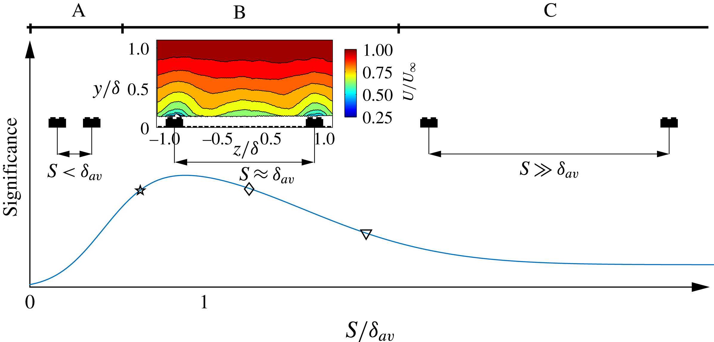
Following the above observation, a hypothetical evolution of ‘significance’ of the secondary motions can be sketched in order to illustrate the effect of the heterogeneity on boundary-layer flows. In figure 1, the flow is separated into three different regimes. In regime A, the secondary flows are small enough such that they are confined in the roughness sublayer. In this case, the outer flow would still remain ‘homogeneous’ along the span. In this case, we expect outer-layer similarity to hold for the mean flow and turbulence quantities. In regime B, secondary flows are expected to occupy a big portion of the primary flow and their effect is expected to extend through the entire boundary layer. Here, the flow is highly three-dimensional and it is unclear if local similarity will hold. Finally, regime C is topographically sparse and can be considered a combination of the two first regimes with a homogeneous region far from the hills (or the wall-drag discontinuities) and a heterogeneous region when close enough to the hills (or the wall-drag discontinuities). The extent of these regimes is rather difficult to assess as this would require extensive and detailed investigations of several parameters that can affect the secondary flows (e.g. the spanwise spacing, the shape and the height of the surface elevation and the Reynolds number), which is beyond the scope of the present investigation. However, in the current study, we aim to examine regime B in detail to understand the influence of surface variations on mean flow and turbulence characteristics. The specific values of
 $S/\unicode[STIX]{x1D6FF}_{av}$
explored in the current paper are marked as symbols in figure 1.
Hypothetical evolution curve of the secondary flow size/strength as a function of the spanwise spacing, inspired from Vanderwel & Ganapathisubramani (Reference Vanderwel and Ganapathisubramani2015). Regimes A, B and C are representative of homogeneous, heterogeneous and transitional surfaces respectively. Symbols represent values of
 $S/\unicode[STIX]{x1D6FF}_{av}$
explored in the present study.

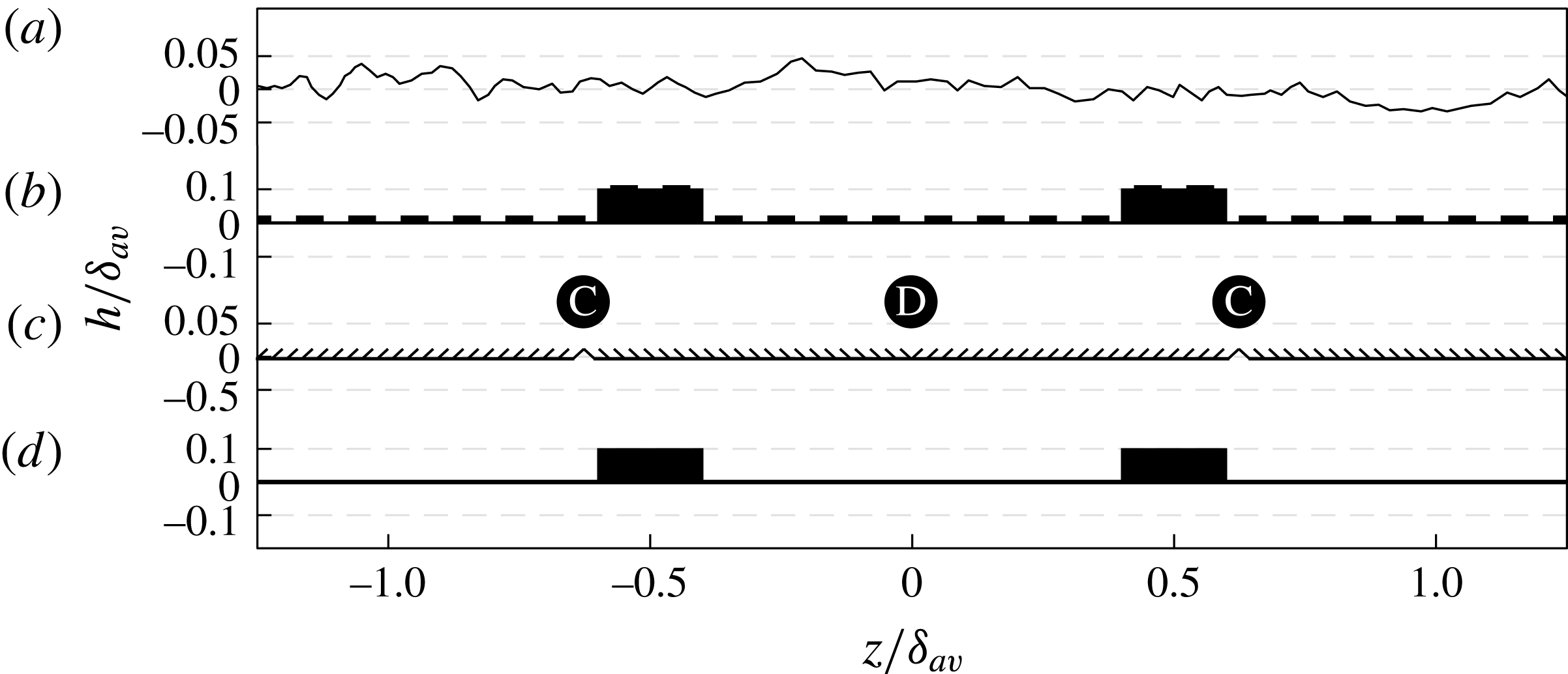
Comparison of spanwise cross-sections from different studies: (a) Wu & Christensen (Reference Wu and Christensen2007) and Barros & Christensen (Reference Barros and Christensen2014), (b) Vanderwel & Ganapathisubramani (Reference Vanderwel and Ganapathisubramani2015), (c) Kevin et al. (Reference Kevin, Monty, Bai, Pathikonda, Nugroho, Barros, Christensen and Hutchins2017) and (d) present study.

A challenging aspect of this study is to reconcile the secondary flows from the two different categories of surfaces discussed above (i.e. surface elevation variations and surface shear-stress variations). In fact, several studies revealed the existence of the secondary motions generated over different surface conditions as shown in figure 2, which suggests the existence of different mechanisms responsible for such large modification of the primary flow. Kevin et al. (Reference Kevin, Monty, Bai, Pathikonda, Nugroho, Barros, Christensen and Hutchins2017) discussed how different types of surfaces can exhibit secondary flows and proposed a classification based on the local isotropy/anisotropy of the skin-friction coefficient
 $C_{f}$
. However, in addition to their classification, a different configuration can also be defined based on surface elevation variations, which also would indirectly lead to variations in local
 $C_{f}$
.
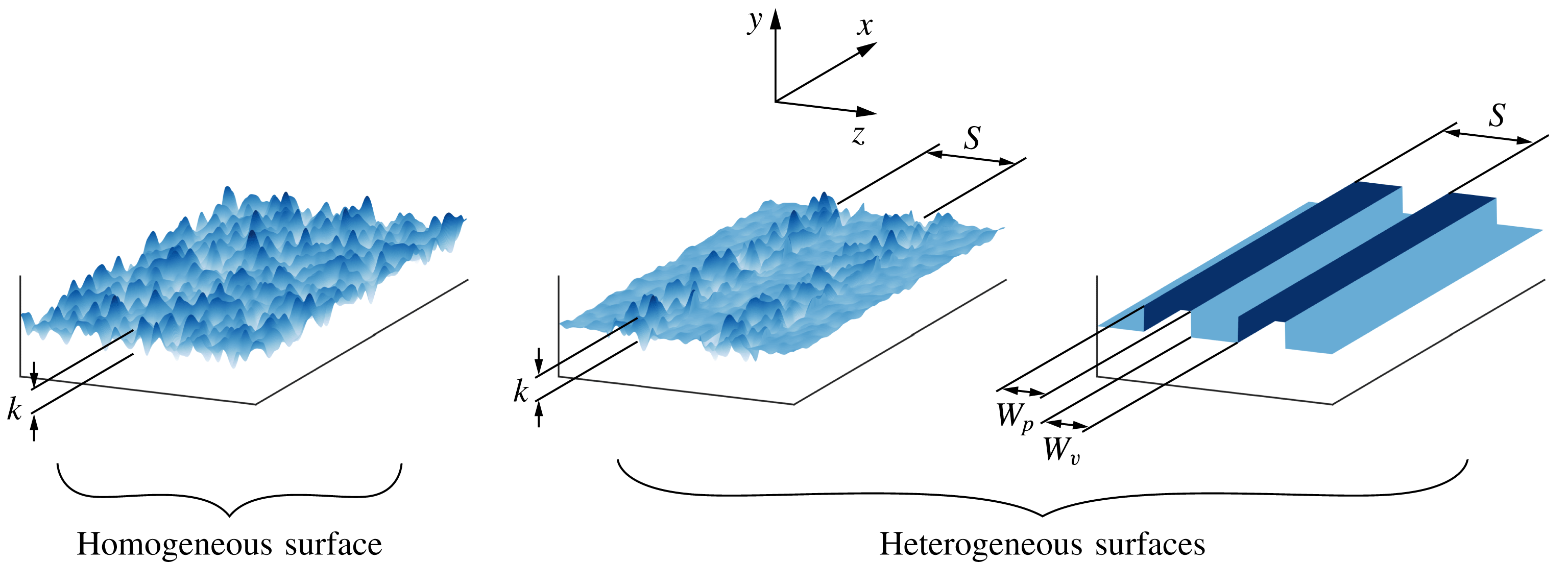
Comparison of homogeneous rough, heterogeneous rough and smooth surfaces. There are three related length scales that define heterogeneity: the width of the peak or ‘high’ roughness (
 $W_{p}$
), the width of the valley or ‘low’ roughness (
 $W_{v}$
) and the spacing between adjacent valleys (
 $S$
).

Considering this classification based on just the surface geometry, then the parameters responsible for the heterogeneity are the width of the peak and the width of the valley (and consequently the spacing between adjacent peaks/valleys since
 $S=W_{p}+W_{v}$
) with
 $W_{p}$
and
 $W_{v}$
representing the equivalent ‘high’ and ‘low’ roughness, respectively, as investigated by Willingham et al. (Reference Willingham, Anderson, Christensen and Barros2014), and shown in figure 3. In this case, if the surfaces present protrusions, there are difficulties in determining the local
 $C_{f}$
which precludes direct determination of the validity of the similarity hypothesis. In fact, Wu & Christensen (Reference Wu and Christensen2007) found that outer-layer similarity was satisfied by the same surfaces that later on were found to exhibit secondary flows (Mejia-Alvarez & Christensen Reference Mejia-Alvarez and Christensen2013; Barros & Christensen Reference Barros and Christensen2014). However, it is critical to note that Wu & Christensen (Reference Wu and Christensen2007) estimated the skin friction through indirect methods (using the Reynolds shear-stress profile). It is unclear if this finding was a result of this indirect method or if surfaces with roughness heterogeneities indeed follow local outer-layer similarity in the mean flow and turbulence statistics. In order to examine this in more detail, we use streamwise strips of elevated smooth surfaces (height
 $h$
) mounted at different spanwise spacings on a baseline smooth surface. This enabled us to generate heterogeneous surfaces with different spacings (with constant
 $W_{p}$
and
 $h$
, and with varying
 $W_{v}$
and consequently
 $S$
). These streamwise constant, spanwise heterogeneous smooth surfaces do not experience any pressure drag from the roughness (since there are no rough protrusions) and will only experience viscous stress. This viscous stress will vary along the span due to the heterogeneities resulting from the topographical variations. This variation in viscous stress can be measured locally using the OFI technique. This allows us to measure the spatial variation of local skin friction using this independent method and use these values to reconcile the mean flow and turbulence statistics that were measured at the same locations using hot-wire anemometry. Overall, this will provide us with an unambiguous assessment of the validity of outer-layer similarity in the flow using direct measurements and enable us to identify the applicability and limitations of these similarity laws in flows over heterogeneous surfaces.
3 Experimental methodology
3.1 Facility
The experimental investigations are conducted in an open-circuit suction wind tunnel at the University of Southampton. The wind tunnel has a working section with a 0.9 m
 $\times$
0.6 m cross-plane
 $(y,z)$
of 4.5 m length. A turbulent boundary layer is developed over a flat plate that is positioned 0.15 m above the wind tunnel test section floor. The boundary layer is tripped 50 mm from the leading edge using a zig–zag turbulator tape of 6 mm point-to-point and 0.5 mm thickness. Further details of the flat plate can be found in the work of Dogan, Hanson & Ganapathisubramani (Reference Dogan, Hanson and Ganapathisubramani2016). In order to assess the skin friction at the measurement location, the smooth boundary-layer plate was equipped with a recessed slot of 0.2 m
 $\times$
0.2 m, where a flat glass plate was inserted. The glass plate was fixed with wax to prevent air leaks as well as to eliminate vibrations during operation.
The free stream velocity generated can reach up to
 $30~\text{m}~\text{s}^{-1}$
, with a turbulence intensity less than 0.5 %, and is controlled through a National Instruments Data-Acquisition system (NI-DAQ) and acquired using a FC510 manometer. To account for the air density variations, the temperature is also acquired, and its standard deviation for an average run (1.5–2.5 h for the boundary-layer profiles and 10–15 min for the skin-friction measurements) is less than
 $0.25\,^{\circ }$
C. Prior to the measurement campaign, a zero-pressure gradient is established to cover the range of the velocities, which is assessed by traversing the pitot probe in the streamwise direction, resulting in an acceleration parameter
 $K=(\unicode[STIX]{x1D708}/U_{\infty }[\text{d}U_{\infty }/\text{d}x])$
less than
 $3\times 10^{-8}$
.
In order to model the spanwise surface elevation, a rectangular smooth foam tape (Self Adhesive EPDM Blend Sealing Strip) with a cross-section
 $h\times W$
of 5 mm
 $\times$
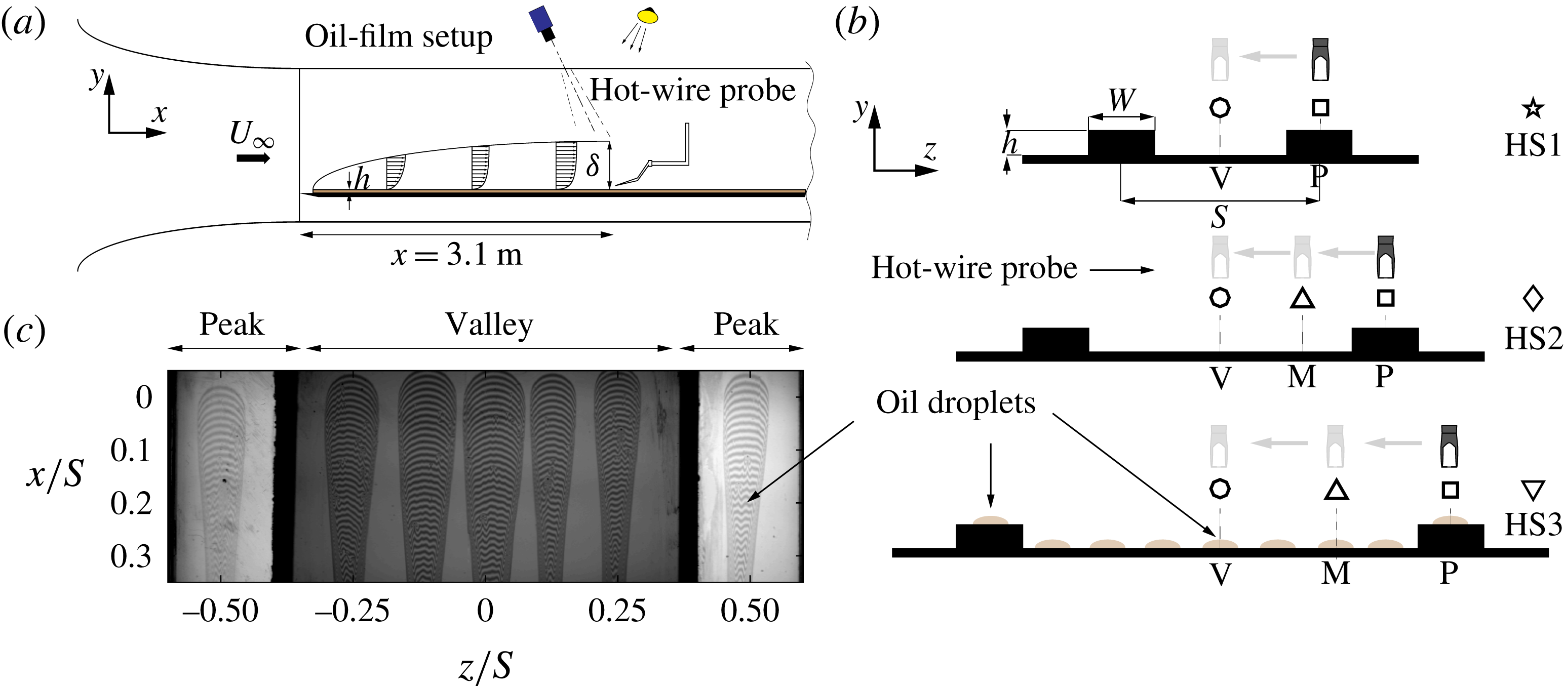
20 mm is chosen. The longitudinal strips are used to create the surface heterogeneity by varying the spacing between adjacent strips by 40, 80 and 160 mm as shown in figure 4(b), such that
 $0.8\leqslant S/\unicode[STIX]{x1D6FF}_{av}\leqslant 3.2$
, where
 $\unicode[STIX]{x1D6FF}_{av}$
in the present study represents an approximation of the spanwise-averaged boundary-layer thickness measured from the hot-wire profiles along the span. These spacings will be referred to as cases HS1, HS2 and HS3, respectively. The surface texture of the foam tape was scanned and its roughness
 $R_{a}$
was found to be less than
 $30~\unicode[STIX]{x03BC}\text{m}$
, which represents a ratio of the roughness to the viscous length scale,
 $RaU_{\unicode[STIX]{x1D70F}}/\unicode[STIX]{x1D708}$
, of less than 2 wall units (at the highest Reynolds number examined in this study), therefore it can be considered to be a hydrodynamically smooth strip.
3.2 Oil-film interferometry
Oil-film interferometry is a direct measurement tool for skin friction, which was first introduced by Squire (Reference Squire1961) and subsequently applied by Tanner & Blows (Reference Tanner and Blows1976) in a flat wall turbulent boundary layer. Since then, many researchers have tested its applicability in different problems including three-dimensional flows (Pailhas et al. Reference Pailhas, Barricau, Touvet and Perret2009; Akomah, Hangan & Naughton Reference Akomah, Hangan and Naughton2011). Several reviews on this technique can be found in the literature, see e.g. Naughton & Sheplak (Reference Naughton and Sheplak2002) and Ruedi et al. (Reference Ruedi, Nagib, Österlund and Monkewitz2003) and more recently Chauhan, Ng & Marusic (Reference Chauhan, Ng and Marusic2010). This method is based upon the relationship between the thinning with time of an oil film deposited on the test surface subjected to a tangential force exerted by the air on the wall, which is represented by the local wall shear stress.
Oil droplets (Dow Corning 200 Silicone oil) that are approximately 6 mm wide are deposited at various locations along the spanwise direction. At the valley, the droplets are positioned in the bottom glass plate. For the peak, a streamwise section of the foam tape (50 mm long) is replaced by a glass plate (and sealed with wax) of the same width and height. The droplets are positioned on top of this glass plate. Inside the measurable area of the droplet (
 ${\approx}50\,\%$
of the droplet area), the statistical uncertainty in
 $C_{f}$
is less than 2 %. Therefore, these droplets provide separate measurements of skin friction and will enable us to assess the spanwise variation of skin friction. A sodium lamp with a wavelength of 589 nm is used to illuminate the oil in order to generate the interferograms. The oil viscosity is calibrated for a wide range of temperatures using a DHR 3 TA Instruments rheometer and the flow temperature is monitored during the measurements. In order to capture the OFI images as illustrated in figure 4(a), a LaVision Imager LX 16 MPixel CCD camera with a pixel size of
 $7.4~\unicode[STIX]{x03BC}\text{m}\times 7.4~\unicode[STIX]{x03BC}\text{m}$
was used. A Nikon 200 mm AF Micro lens was fitted to the camera alongside a Scheimpflug adapter to account for the camera view angle. This resulted in a field of view of 50 mm
 $\times$
100 mm in the
 $(x,z)$
-plane as shown in figure 4(c).
A series of 100 interferograms per spacing and speed are acquired for approximately 10 min in each run using LaVision DAVIS 8.2. The latter is also used to calibrate the camera and for de-warping the images through a third-order polynomial. The interferograms are then post-processed using the method described by Blay Esteban et al. (Reference Blay Esteban, Dogan, Rodríguez-Lopéz and Ganapathisubramani2017). The current results of the relative uncertainty in the skin-friction velocity based on the smooth-wall correlation of Nagib, Chauhan & Monkewitz (Reference Nagib, Chauhan and Monkewitz2007) are less than 2.5 %.
(a) Side view of the experimental set-up including the hot-wire anemometry and oil-film interferometry. (b) Schematics of the three spacings (HS1:
 $S/\unicode[STIX]{x1D6FF}_{av}\approx 0.8$
, HS2:
 $S/\unicode[STIX]{x1D6FF}_{av}\approx 1.7$
and HS3:
 $S/\unicode[STIX]{x1D6FF}_{av}\approx 3.2$
) and the spanwise reference points V, M and P representative of the valley, mid-valley peak and the peak locations. (c) Example of de-warped interferograms at
 $20~\text{m}~\text{s}^{-1}$
for the HS2 case. Throughout this paper, the star, diamond and down-pointing triangle symbols will refer to HS1, HS2 and HS3 respectively used to present the OFI results, while the circle, up-pointing triangle and square symbols are used to refer to the valley, mid-valley peak and peak locations in the hot-wire results. The colours are used to show the Reynolds number effect.

3.3 Hot-wire anemometry
A single hot-wire boundary-layer-type probe is used in order to measure the time series of the streamwise velocity at different wall-normal locations and to determine the mean velocity profiles. The probe is also traversed in the spanwise direction in order to obtain additional information due to the heterogeneity of the flow herein studied. As shown in figure 4(b), these stations are represented by P, M and V which refer to the peak, mid-peak valley and valley locations, which coincide respectively with the spanwise-normalized distance
 $z/S=0.5$
, 0.25 and 0, except for HS1 spacing case, where the profiles were only acquired at P and V locations. The single wire probe had a 10 mm long prongs spanned by a 3 mm long and
 $5~\unicode[STIX]{x03BC}\text{m}$
diameter tungsten wire with a sensing length of about 1 mm. The resulting length-to-diameter ratio of the probe is 200 which follows the recommendation of Hutchins et al. (Reference Hutchins, Nickels, Marusic and Chong2009). A DANTEC Streamline Pro constant temperature anemometer (CTA) system was used and operated at fixed overheat ratio of 0.8. The turbulent boundary-layer profiles consisted of 42 wall-normal locations, each of which has an acquisition time of 3–5 min with a sampling rate of 25–70 kHz and low-pass filtered at 10 kHz to 30 kHz depending on the free stream velocity, allowing the convergence of streamwise turbulence intensity and the spectra.
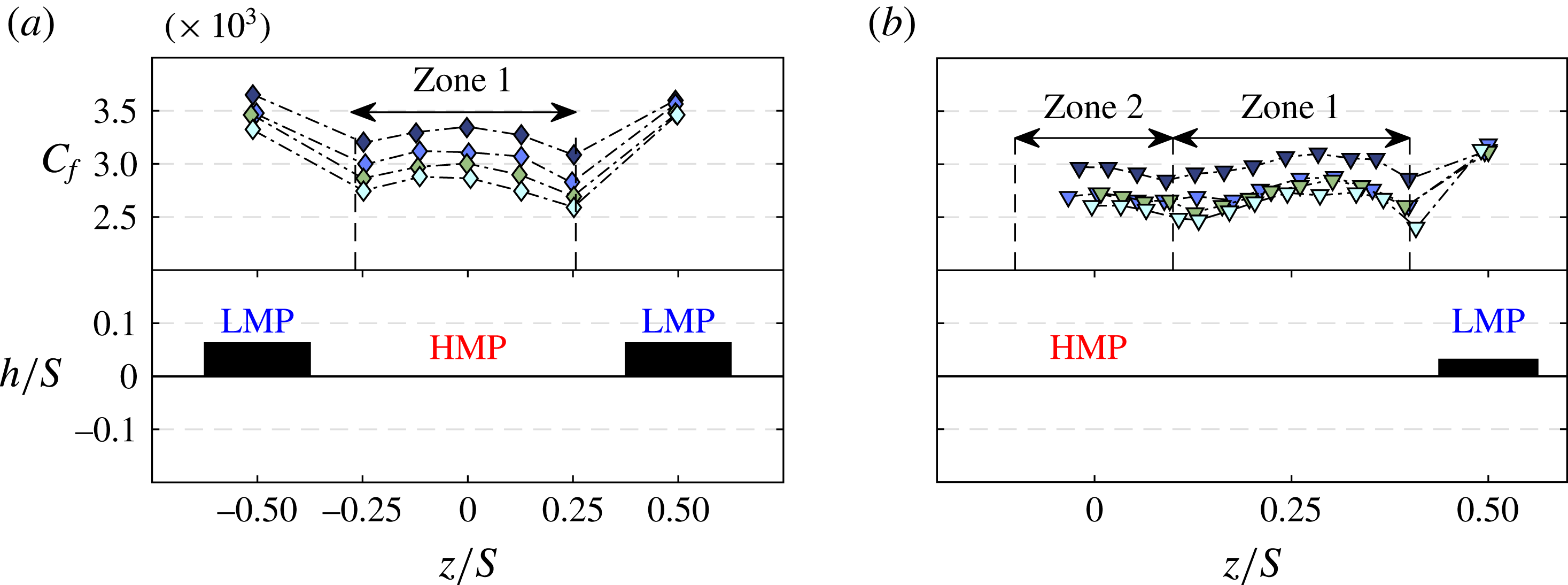
Spanwise variation of the skin-friction coefficient subjected to different spacings at different unit Reynolds numbers (

 $Re_{x}=2\times 10^{6}$
, (b)
 $Re_{x}=4\times 10^{6}$
.

4 Results
4.1 The mean surface shear stress
A critical part of the analysis of a turbulent boundary layer is the accurate assessment of the friction velocity, since most of the analysis is based upon this quantity. The following results from the OFI method describe the response of the surface shear stress to the presence of a surface heterogeneity. Figure 5 shows the spanwise distribution of the local skin-friction coefficient for the different spacings at two Reynolds numbers (
 $Re_{x}=U_{\infty }x/\unicode[STIX]{x1D708}$
, where
 $x$
is the distance to the measurement location from leading edge) obtained for two different free stream velocities. As expected for a higher Reynolds number, the skin-friction coefficient is lower. At low Reynolds number, the values of
 $C_{f}$
for the HS1 and HS2 surfaces are greater than the smooth-wall value with the HS1 surface producing the most viscous drag. Interestingly, the measurements of the HS3 surface indicate a potential drag reduction within the valley. The variation of
 $C_{f}(z)$
across the span differs significantly due to the surface heterogeneity. This result can be interpreted as a consequence of a global change in the mean flow due to the presence of secondary flows (as observed by Vanderwel & Ganapathisubramani (Reference Vanderwel and Ganapathisubramani2015)), which in turn leads to local modifications of the skin friction. From figure 5, we observe that the skin friction is higher on the elevated region of the surface compared to the rest of the valley area. This indicates that the mean velocity gradient at the wall
 $\text{d}U/\text{d}y$
is higher at the elevated surface compared to the valley, which is a result of the reorganization of the turbulent boundary-layer structure across the cross-plane. As described by Vanderwel & Ganapathisubramani (Reference Vanderwel and Ganapathisubramani2015), the secondary flows create HMPs in the valleys and LMPs along the elevated region of the surface. This in turn leads to the spatial heterogeneity in the skin friction. Interestingly, as shown in figure 5, the previous observation leads to a counter-intuitive result, that the skin friction is higher at the location of the LMP compared to that at the valley.
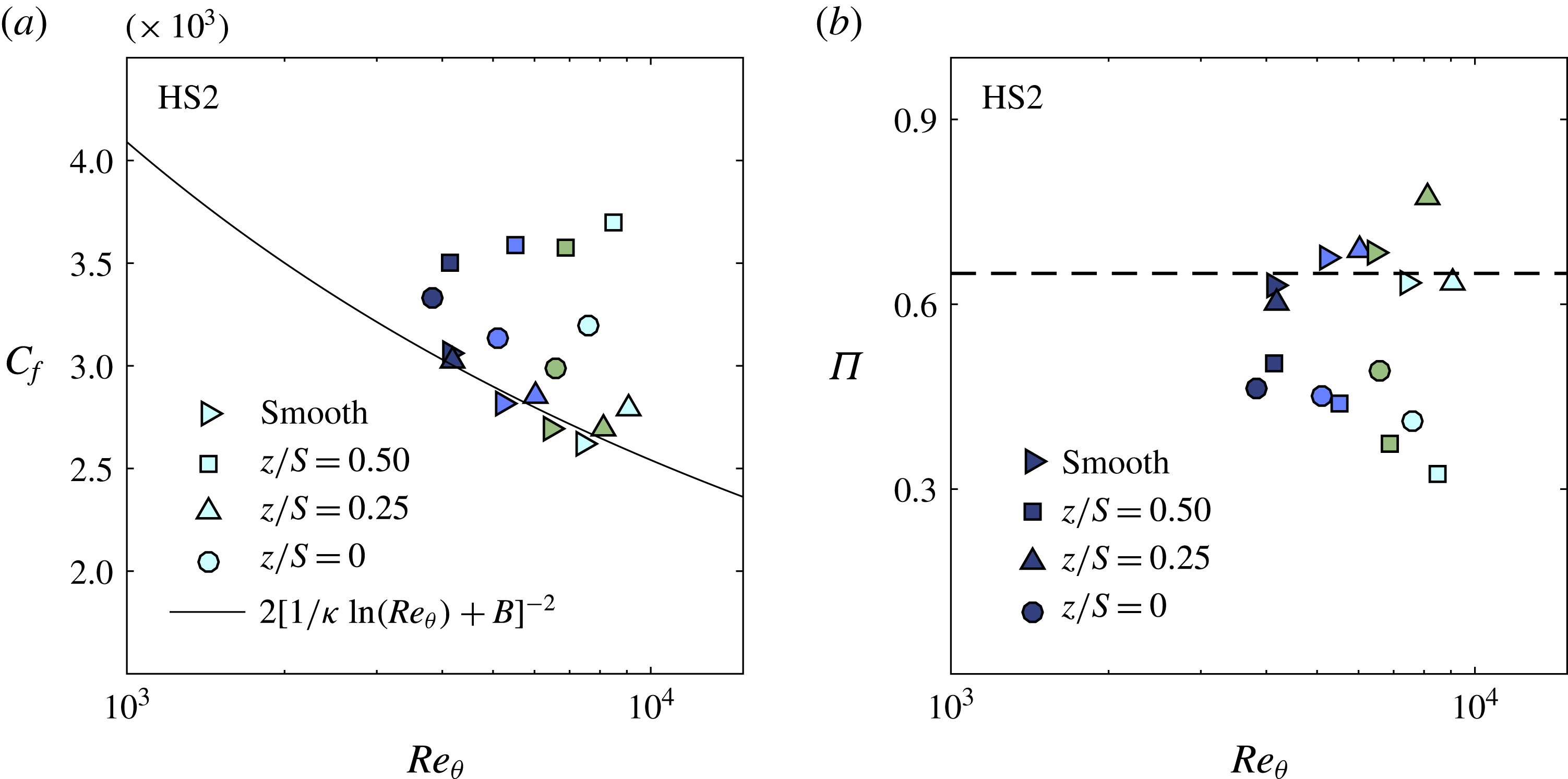
Figure 6 shows the effect of Reynolds number on the spanwise distribution of
 $C_{f}(z)$
for both the HS2 and HS3 spacings. We notice that the reduction in
 $C_{f}$
with Reynolds number is higher in the valley (HMP) compared to the surface elevation (LMP), which consistently holds for all the cases (including HS1). This behaviour indicates the existence of different activities in the LMPs and HMPs promoted by potential secondary flows that lead to a Reynolds number effect. The response of the spanwise distribution of the skin friction
 $C_{f}(z)$
to HS2 and HS3 seems to follow a wavy type of behaviour with a different shape and magnitude. For HS2, a bump in the skin-friction distribution is formed with a local maximum (at the valley centre) observed at
 $z/S=0$
, then decays when getting close to the surface elevation. This region is labelled Zone 1 as illustrated in figure 6(a). For HS3 (as shown in figure 6
b), two different zones can be observed. These zones can be identified as the regions between local minima in the spanwise distribution of
 $C_{f}$
. The first zone extends from the edge of the surface elevation up to
 $z/S\approx 0.1$
and is similar to Zone 1 found for HS2. The second zone appears in the centre of the valley and spans from
 $z/S=-0.1$
to 0.1. These patterns (and zones) are also consistent with the locations of the HMPs and LMPs observed by Vanderwel & Ganapathisubramani (Reference Vanderwel and Ganapathisubramani2015). The region labelled Zone 1 can be presumed to be the extent of the HMP induced by two counter-rotating rolling modes flanking the surface elevation. This region exists for both HS2 and HS3. However, Zone 2 for HS3 could be considered an effect of a tertiary flow (as identified by Vanderwel & Ganapathisubramani Reference Vanderwel and Ganapathisubramani2015) and is likely to be induced at the centre of the valley due to the larger value of
 $S/\unicode[STIX]{x1D6FF}_{av}$
.
Spanwise distribution of the skin-friction coefficient and observation of the potential secondary and tertiary flow signatures represented by Zone 1 and Zone 2 respectively for (a) HS2 and (b) HS3 spacings, at different Reynolds numbers; (▾, grey):
 $2\times 10^{6}$
, (▾, blue):
 $3\times 10^{6}$
, (▾, green):
 $3.9\times 10^{6}$
(▾, light blue):
 $4.9\times 10^{6}$
.

(a)
 $\unicode[STIX]{x1D6E4}_{1}$
and (b)
 $\unicode[STIX]{x1D6E4}_{2}$
plots illustrating respectively the global and local heterogeneity in the skin friction as defined in (4.1). (c) Spanwise-averaged skin-friction coefficient normalized with the smooth-wall data varying across the spacings at different Reynolds number, (


Following these observations, it is evident that when a turbulent boundary layer grows over a spanwise heterogeneous surface, it not only leads to large-scale flow field modifications, but also affects the surface stress distribution and the total drag generated by these surfaces will depend on the length scale of the heterogeneity. Following the previous results, we attempt to quantify the variation in surface stress with surface heterogeneities in different ways. Figure 7(a,b) shows the ratios, defined as
 $$\begin{eqnarray}\displaystyle \unicode[STIX]{x1D6E4}_{1}=\frac{\displaystyle \frac{1}{W_{p}}\int _{-W_{p}/2}^{W_{p}/2}C_{f}(z)\,\text{d}z|_{peak}}{\displaystyle \frac{1}{W_{v}}\int _{-W_{v}/2}^{W_{v}/2}C_{f}(z)\,\text{d}z|_{valley}}-1,\quad \unicode[STIX]{x1D6E4}_{2}=\frac{C_{f}(z=z_{peak})}{C_{f}(z=z_{peak}+W)}, & & \displaystyle\end{eqnarray}$$
where
 $\unicode[STIX]{x1D6E4}_{1}$
can be considered a global measure of flow heterogeneity which also enables us to quantify the amount of viscous drag produced by the low- and high-momentum pathways at different Reynolds numbers across different spacings. As an alternative measure,
 $\unicode[STIX]{x1D6E4}_{2}$
determines the ratio of the skin friction at the surface elevation over the skin friction at an equivalent distance from the peak when normalized by the width of the strip, which can be considered a measure of a local flow heterogeneity.
 $\unicode[STIX]{x1D6E4}_{1}$
and
 $\unicode[STIX]{x1D6E4}_{2}$
appear to both depend on the Reynolds number (
 $Re_{x}$
) and spanwise spacing. Both quantities appear to systematically be higher for HS1 and decreases with increasing spacing (HS2 and HS3) with slightly higher values of
 $\unicode[STIX]{x1D6E4}_{2}$
for the HS2 and HS3 cases. As mentioned before, the variation of skin friction with Reynolds number is different for peaks and valleys, which translates to higher relative drag at the peak compared to the valley at high Reynolds number. It should be noted that the value of
 $\unicode[STIX]{x1D6E4}_{1}$
does not account for any effects caused by differences in the ratio of the width of peak to the spacing. In fact,
 $W_{p}/S$
varies between the cases (0.5, 0.25 and 0.125 respectively for HS1, HS2 and HS3) which can have an effect on the organization of the LMPs and HMPs, which consequently can affect the wall drag.
The spanwise-averaged skin friction was determined as
 $$\begin{eqnarray}\displaystyle C_{F}=\frac{1}{S}\int _{-S/2}^{S/2}C_{f}(z)\,\text{d}z & & \displaystyle\end{eqnarray}$$
and was evaluated at different Reynolds numbers and for different spacings. Figure 7(c) shows measurements of
 $\unicode[STIX]{x1D6FD}=(C_{F}/C_{f_{smooth}})-1$
, which represents a measure of the drag increase due to the surface heterogeneity. The value of
 $\unicode[STIX]{x1D6FD}$
was typically higher for the HS1 surface, whereas the HS2 and HS3 surfaces have relatively lower values. It monotonically increases from low to high Reynolds numbers for the HS2 and HS3 cases, but shows a sudden drop for HS1. The reason for the sudden drop at the highest Reynolds number for HS1 is due to the decrease in
 $C_{f}$
measured in the valley, which is also observed in figure 7(a). Additionally, figure 7(c) also shows a negative value at low Reynolds numbers for HS3. This result indicates a potential drag reduction behaviour, however, the difference (skin-friction reduction) is of the order of the uncertainty of the measurements.
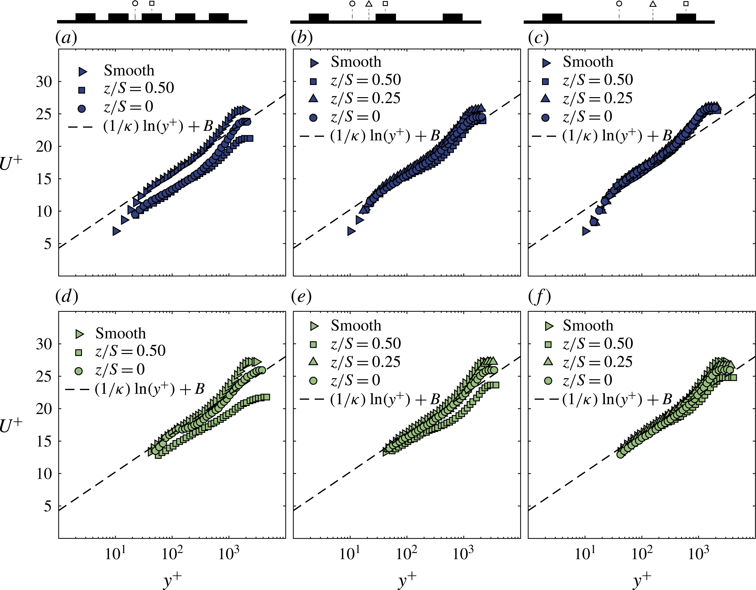
Inner scaling of the local velocity profiles for the (a,d) HS1, (b,e) HS2 and (c,f) HS3 spacings at (a–c)
 $Re_{x}=2\times 10^{6}$
and (d–f)
 $Re_{x}=3.9\times 10^{6}$
. The values of the log-law slope
 $\unicode[STIX]{x1D705}$
and the smooth-wall intercept
 $B$
used in this study are 0.387 and 4.29 respectively.

4.2 Mean velocity profiles
The mean streamwise velocity with the wall-normal location profiles are scaled with inner variables,
 $U_{\unicode[STIX]{x1D70F}}$
for
 $U$
and
 $\unicode[STIX]{x1D708}/U_{\unicode[STIX]{x1D70F}}$
for
 $y$
, and plotted with the
 $^{+}$
symbol in figure 8. It is important to clarify the origin for the wall-normal direction as this is a source of contention in many studies of rough-wall flows. For the current study, the vertical origin was deliberately defined as the location of the wall. Therefore, the origin for valley profiles is at the bottom of the valley while for the peak profiles, the origin is located at the peak. This will allow us to compare the near-wall and outer-scaling laws at different spanwise locations. Figure 8 shows the effect of spacing in columns and Reynolds number in rows. All profiles seem to show the existence of a log layer in the mean velocity profiles for different spanwise locations. At low Reynolds number, the hot-wire resolves the near-wall layer (buffer layer) down to 10 wall units. A good collapse in the near wall of the profiles can be seen for HS2 and HS3. However, inner-scaled velocity profiles seem to be more variable for HS1, observed both at the near wall and the wake part of the boundary layer. A downward shift can be observed accompanied with a different wake strength for both locations
 $z/S=0.5$
and
 $z/S=0$
. The wake seems to be weaker at the surface elevation and stronger at the valley. The mean velocity profiles show a trend that is similar to the skin friction where the mean flow is strongly affected by the heterogeneity for HS1, then the flow starts recovering towards the smooth wall for HS2 and HS3. This is confirmed in figure 8(d–f) at higher Reynolds number. The wake strength appears to be weakening for the profiles at the peaks. From previous studies, the peaks coincide with the LMPs which are dominated by an upwash motion that increases the turbulence activity across the boundary layer, which can result in a lower activity of intermittency at the peak.
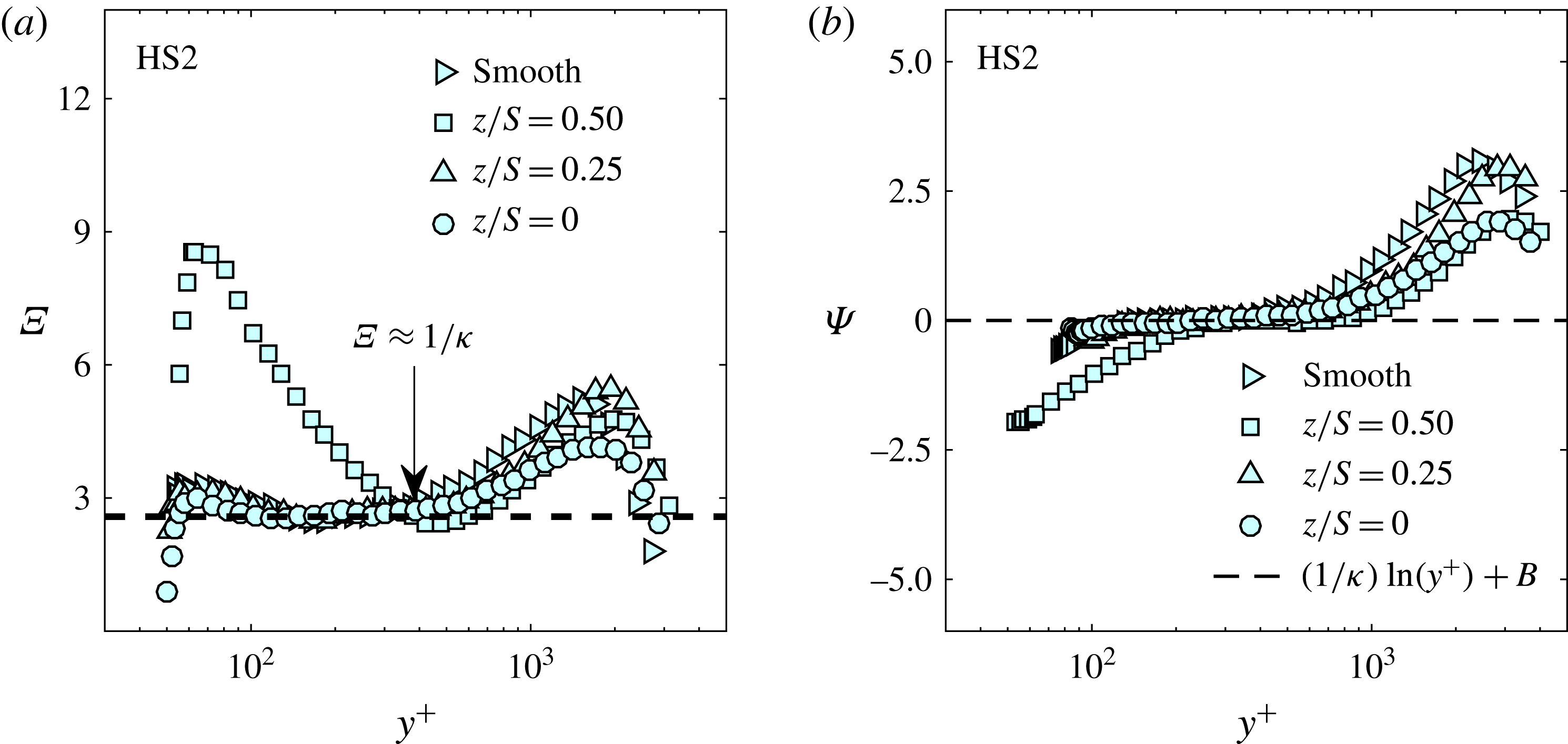
(a) Variation of the indicator function
 $\unicode[STIX]{x1D6EF}$
and (b) variation of the
 $\unicode[STIX]{x1D6F9}$
function for different spanwise locations at the highest Reynolds number for the HS2 case. In the present study, a second-order central-difference scheme was used in order to obtain
 $\unicode[STIX]{x1D6EF}$
.

Surface roughness is known to induce a vertical and a horizontal shift in the mean velocity profiles as shown in figure 8 resulting from both a roughness function (
 $\unicode[STIX]{x0394}U^{+}$
) and a zero-plane displacement (
 $d$
). We deduce
 $d$
from a modified indicator function by taking the derivative of (2.1) with respect to
 $y$
, which leads to:
 $$\begin{eqnarray}\displaystyle \unicode[STIX]{x1D6EF}=(y^{+}-d^{+})\frac{\text{d}U^{+}}{\text{d}y^{+}}=\frac{1}{\unicode[STIX]{x1D705}}. & & \displaystyle\end{eqnarray}$$
This form is usually used to identify the existence of a log layer in the mean velocity profile and the determination of the log-layer slope,
 $1/\unicode[STIX]{x1D705}$
, for smooth walls (Österlund et al.
Reference Österlund, Johansson, Nagib and Hites2000; Segalini, Örlü & Alfredsson Reference Segalini, Örlü and Alfredsson2013). In the present study
 $1/\unicode[STIX]{x1D705}\approx 2.58$
was fixed and
 $d^{+}$
is found to be the value that minimizes the difference
 $\unicode[STIX]{x1D6EF}$
–
 $1/\unicode[STIX]{x1D705}$
in the plateau of
 $\unicode[STIX]{x1D6EF}$
as shown in figure 9(a). Once the zero-plane displacement is determined, the log-layer profiles are subtracted from the inner-normalized mean velocity profile to obtain a quantity,
 $\unicode[STIX]{x1D6F9}$
,
 $$\begin{eqnarray}\displaystyle \unicode[STIX]{x1D6F9}=U^{+}-\frac{1}{\unicode[STIX]{x1D705}}\ln (y^{+}-d^{+})-B+\unicode[STIX]{x0394}U^{+}. & & \displaystyle\end{eqnarray}$$
Figure 9(b) shows the profiles of
 $\unicode[STIX]{x1D6F9}$
for different locations. In the log region, the value of
 $\unicode[STIX]{x1D6F9}$
is approximately zero for the appropriate value of
 $\unicode[STIX]{x0394}U^{+}$
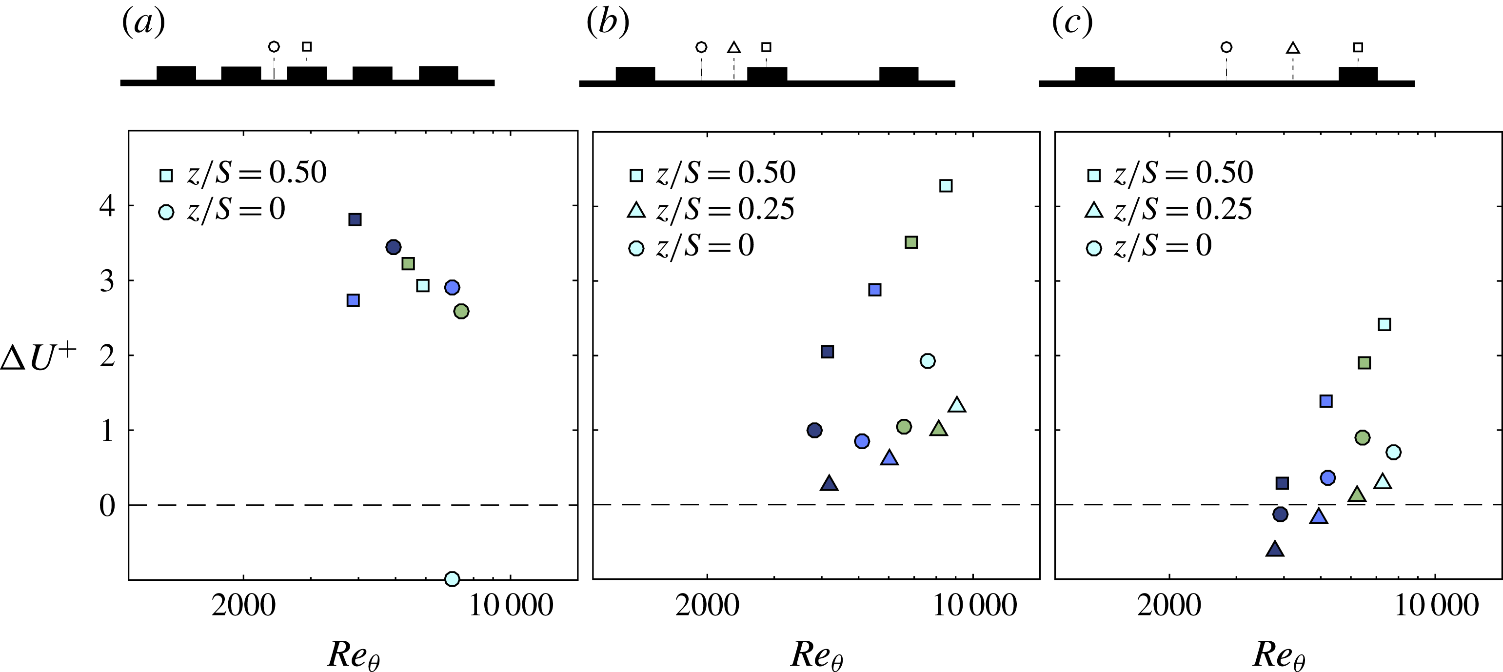
. This procedure is repeated for all spacings and locations over a range of Reynolds numbers. The range of
 $\unicode[STIX]{x0394}U^{+}$
obtained for the three cases for the different Reynolds numbers spans from
 $-$
1 to 4.3 as illustrated in figure 10. There is no clear trend in the values of
 $\unicode[STIX]{x0394}U^{+}$
for HS1 at the peak and valley. However, it is clear that for HS1
 $\unicode[STIX]{x0394}U^{+}$
is higher at the peak than the valley. For the HS2 and HS3 cases, a monotonic increase in
 $\unicode[STIX]{x0394}U^{+}$
for the peak locations is observed, while, at the valley there are different trends with
 $Re_{\unicode[STIX]{x1D703}}$
(
 $Re_{\unicode[STIX]{x1D703}}=U_{\infty }\unicode[STIX]{x1D703}/\unicode[STIX]{x1D708}$
with
 $\unicode[STIX]{x1D703}$
representing the momentum thickness). Additionally, it is apparent that with increasing spacing, the roughness function and the roughness effects tend to decrease as observed in figure 7(c) which also showed the impact of the spanwise spacing in the total drag produced by these surfaces. In fact, for HS3, the values of
 $\unicode[STIX]{x0394}U^{+}$
appears to be negative for lower Reynolds numbers (especially for
 $z/S=0$
and 0.25), which could be interpreted as local drag reduction.
Evolution of the roughness function with Reynolds number based on the momentum thickness
 $Re_{\unicode[STIX]{x1D703}}$
at different spanwise locations, for (a) HS1, (b) HS2 and (c) HS3, with the
 $\unicode[STIX]{x0394}U^{+}$
herein is estimated from the function
 $\unicode[STIX]{x1D6F9}$
. The symbol colours are explained in figure 6.

Variation of (a) local skin-friction coefficient and (b) the wake strength with respect to the Reynolds number based on the momentum thickness for HS2 spacing at different spanwise locations. The black-dashed line represents the average value from the four different Reynolds numbers of the smooth-wall data with
 $\unicode[STIX]{x1D6F1}$
 ${\approx}$
0.65. The symbol colours are explained in figure 6.

In order to further assess the drag of the heterogeneous surfaces, the example of variation of
 $C_{f}$
along the span for the HS2 case compared with a smooth wall is plotted against the local Reynolds number based on momentum thickness (computed from hot-wire data) in figure 11. The figure shows that the smooth-wall OFI data match relatively well with the semi-empirical relation of Nagib et al. (Reference Nagib, Chauhan and Monkewitz2007) (deviation less than 2.5 %). As observed from the measurements of
 $C_{f}(z)$
for the HS2 case at different spanwise locations, the surface tends to create higher drag over the surface elevation than the valley (similar to the results observed from figure 10). At the highest Reynolds number achieved in our facility, the difference in
 $C_{f}$
for
 $z/S=0.5$
and the smooth wall at
 $Re_{\unicode[STIX]{x1D703}}\approxeq 8000$
is approximately 35 %. Different trends seem to exist along the span for HS2. At the peak, the skin friction seems to adopt a monotonic behaviour with a weak positive slope indicating that skin friction increases with Reynolds number. However, a different evolution can be observed for the skin friction at
 $z/S=0$
and
 $z/S=0.25$
. The skin friction is observed to decrease until a certain Reynolds number which then transitions to an increasing
 $C_{f}$
.
An additional way for estimating the roughness function is from the difference between the skin friction of the rough wall from that of a smooth wall at equivalent Reynolds numbers based on the momentum thickness (Hama Reference Hama1954):
 $$\begin{eqnarray}\displaystyle \unicode[STIX]{x0394}U^{+}=\left(\sqrt{\frac{2}{C_{f}}}\right)_{s}-\left(\sqrt{\frac{2}{C_{f}}}\right)_{r}. & & \displaystyle\end{eqnarray}$$
This allows us to obtain an estimate of the roughness function with the advantage that knowledge of the zero-plane displacement is not required. The roughness function evaluated from (4.5) showed consistent trends with comparison to
 $\unicode[STIX]{x0394}U^{+}$
estimated from (4.4), however with differences in magnitude of up to
 $\pm 20\,\%$
. These differences tend to systematically reduce with increasing spacing. The observed quantitative differences are because the
 $\unicode[STIX]{x0394}U^{+}$
estimated from (4.5) is contingent on flow over both the smooth and rough wall exhibiting wake similarity, which translates to a collapse in the mean velocity profiles in defect form. This suggests that the impact of surface heterogeneity on the wake strength
 $\unicode[STIX]{x1D6F1}$
should also be evaluated.
The wake strength depicts the departure of the mean velocity profiles from the logarithmic behaviour and most studies assume that rough and smooth walls have a universal wake parameter (Castro Reference Castro2007), which further feeds into the arguments of outer-layer similarity. In the present study, the wake strength is estimated from the outer part of the mean velocity profile expressed in the defect form as:
 $$\begin{eqnarray}\displaystyle \frac{U_{\infty }-U}{U_{\unicode[STIX]{x1D70F}}}=-\frac{1}{\unicode[STIX]{x1D705}}\ln \left(\frac{y}{\unicode[STIX]{x1D6FF}}\right)+\frac{\unicode[STIX]{x1D6F1}}{\unicode[STIX]{x1D705}}\left[2-w\left(\frac{y}{\unicode[STIX]{x1D6FF}}\right)\right], & & \displaystyle\end{eqnarray}$$
where
 $w$
is the wake function (Coles Reference Coles1956), chosen for the current investigation to be:
 $$\begin{eqnarray}\displaystyle w\left(\frac{y}{\unicode[STIX]{x1D6FF}}\right)=2\sin ^{2}\left[\left(\frac{y}{\unicode[STIX]{x1D6FF}}\right)\frac{\unicode[STIX]{x03C0}}{2}\right]. & & \displaystyle\end{eqnarray}$$
Figure 11(b) illustrates the values of the wake strength obtained for the case of HS2 plotted against
 $Re_{\unicode[STIX]{x1D703}}$
(all values are tabulated in table 1). In the present case, we observe that
 $\unicode[STIX]{x1D6F1}$
is also affected by the spanwise heterogeneity of the surface which shows a weakening of the wake parameter. The smooth wall results are shown to be in agreement with smooth-wall values found in the literature (depending on the choice of the function
 $w$
and
 $(\unicode[STIX]{x1D705},B)$
). Different trends appear for different spanwise locations. At the peak, the value of
 $\unicode[STIX]{x1D6F1}$
is lower and decreases with
 $Re_{\unicode[STIX]{x1D703}}$
. Similar observations can be made for the wake strength measured at the valley, but, relatively the value of
 $\unicode[STIX]{x1D6F1}$
is closer to the smooth wall. This behaviour is however different at
 $z/S=0.25$
, where
 $\unicode[STIX]{x1D6F1}$
is shown to increase initially with Reynolds number and is seen to decrease after a certain Reynolds number. The scatter of the wake strength values not only illustrates the inhomogeneity in the mean flow but also in the turbulence. This also indicates that outer-layer similarity might not exist in these flows, as will be discussed in the following section.
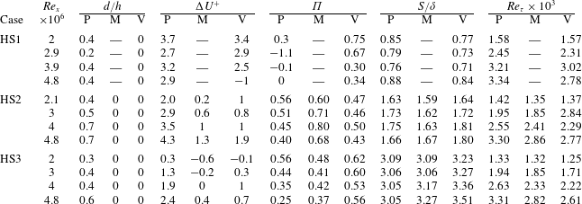
Table 1 summarises the different values of different boundary-layer characteristics for the three cases over a range of Reynolds numbers discussed above. Note that this table also has values of
 $S/\unicode[STIX]{x1D6FF}$
based on the local
 $\unicode[STIX]{x1D6FF}$
estimated from the profiles. However, in the context of secondary flows, it is perhaps suitable to define an average boundary-layer thickness
 $\unicode[STIX]{x1D6FF}_{av}$
and normalize the spacing based on this value. The normalized spacing based on this average value is given in the table caption. This confirms that our cases span the range within regime B in figure 1.
Boundary-layer characteristics for three different heterogeneous surfaces at different spanwise locations for different unit Reynolds numbers with HS1:
 $S/\unicode[STIX]{x1D6FF}_{av}\approx 0.8$
, HS2:
 $S/\unicode[STIX]{x1D6FF}_{av}\approx 1.7$
and HS3:
 $S/\unicode[STIX]{x1D6FF}_{av}\approx 3.2$
.

Outer scaling of the local velocity profiles for the (a,d) HS1, (b,e) HS2 and (c,f) HS3 spacings at (a–c)
 $Re_{x}=2\times 10^{6}$
and (d–f)
 $Re_{x}=3.9\times 10^{6}$
.

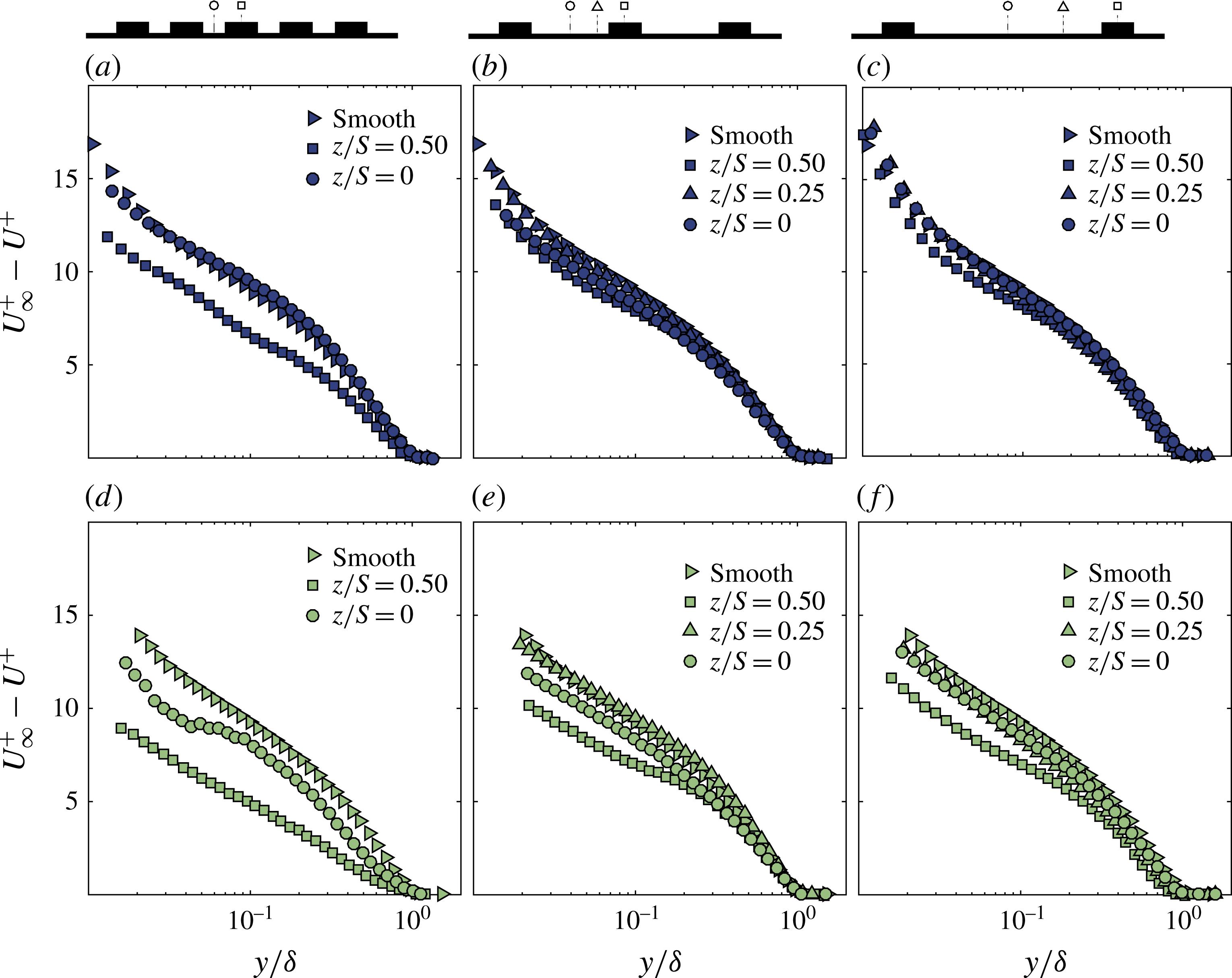
Figure 12 shows the mean velocity profiles in defect form for the three spacings in column at two different Reynolds numbers in rows. Just as previous figures, the vertical origins are local (i.e.
 $y=0$
, where the wall is locally). The boundary-layer thickness
 $\unicode[STIX]{x1D6FF}$
is also local from each profile. It is well established for homogeneous roughness that a collapse with smooth-wall data is observed from
 $0.2\unicode[STIX]{x1D6FF}$
onwards (Jiménez Reference Jiménez2004, Castro Reference Castro2007 and Squire et al.
Reference Squire, Morrill-Winter, Hutchins, Schultz, Klewicki and Marusic2016), meaning that the surface roughness effects (viscous effects) are contained within the near wall, and the rest of the flow behaves as in the case of a smooth wall. However, for heterogeneous surfaces as shown in figure 12(a–f), we can observe a lack of collapse for all the cases. For the surfaces where
 $S$
and
 $\unicode[STIX]{x1D6FF}$
are of the same order of magnitude, such as these, outer-layer similarity of local profiles is not expected to hold. At the peak, a strong deviation of the profiles from the smooth wall can be observed, not only in the magnitude but also in shape. As the spacing increases, the shape of the profile starts to recover as seen for case HS3.
The above observation is consistent with the behaviour of the wake strength, which was shown to vary at different spanwise locations. Additionally, there seems to be a Reynolds number effect on these mean velocity profiles in defect form. As seen in figure 12(e,f), the collapse is worse between two points in the valley (centre of valley,
 $z/S=0$
, and mid-valley-peak point,
 $z/S=0.25$
). In fact, as the Reynolds number increases, the lack of collapse is found to get worse in the outer layer reaching almost the entire boundary-layer thickness regardless of the spacing. This suggests that as Reynolds number increases, the secondary flows grow stronger in the outer region but its effect is not felt to the same extent at the wall. This leads to a lack of collapse in defect profiles, when scaled with a local skin-friction velocity, since the effect is not uniformly proportional across the vertical extent. Perhaps, this is the reason why Wu & Christensen (Reference Wu and Christensen2007) found outer-layer similarity in flows over spanwise heterogeneities. They determined the skin-friction velocity in the outer region (using Reynolds shear-stress method) which could have provided a different estimate that is directly proportional to the strength of the secondary flow. However, this value is not representative of the local surface shear stress. This is also consistent with Nugroho et al. (Reference Nugroho, Hutchins and Monty2013), who indicated that outer-layer similarity cannot hold in the presence of secondary flows due to the occurrence of the upwash and downwash motions.
These defect profiles also indicate why the skin friction is higher at the LMPs rather than the HMPs. The measured skin friction is representative of the viscous shear stress
 $\unicode[STIX]{x1D707}(\text{d}U/\text{d}y)$
. The shape of the boundary layer at
 $z/S=0.5$
seems to be fuller compared to that at
 $z/S=0$
, which is also higher than at
 $z/S=0.25$
. This is an indication of the variation of the velocity gradient at the wall across the span. Therefore the results we previously observed in the spatial distribution of the skin friction are in line with the data provided by the mean velocity profiles. Therefore, from the results presented herein, we observe that outer-layer similarity is not fulfilled when the turbulent boundary layer is perturbed by a surface heterogeneity. Note that all of our cases are in regime B, as indicated in the introduction, where we expect to have secondary flows. As Reynolds number increases, the effect of secondary motions on the mean flow increases, but, its effect on skin friction is perhaps not as strong. Therefore, when scaled appropriately, the lack of collapse is evident.
4.3 Properties of the turbulent flow
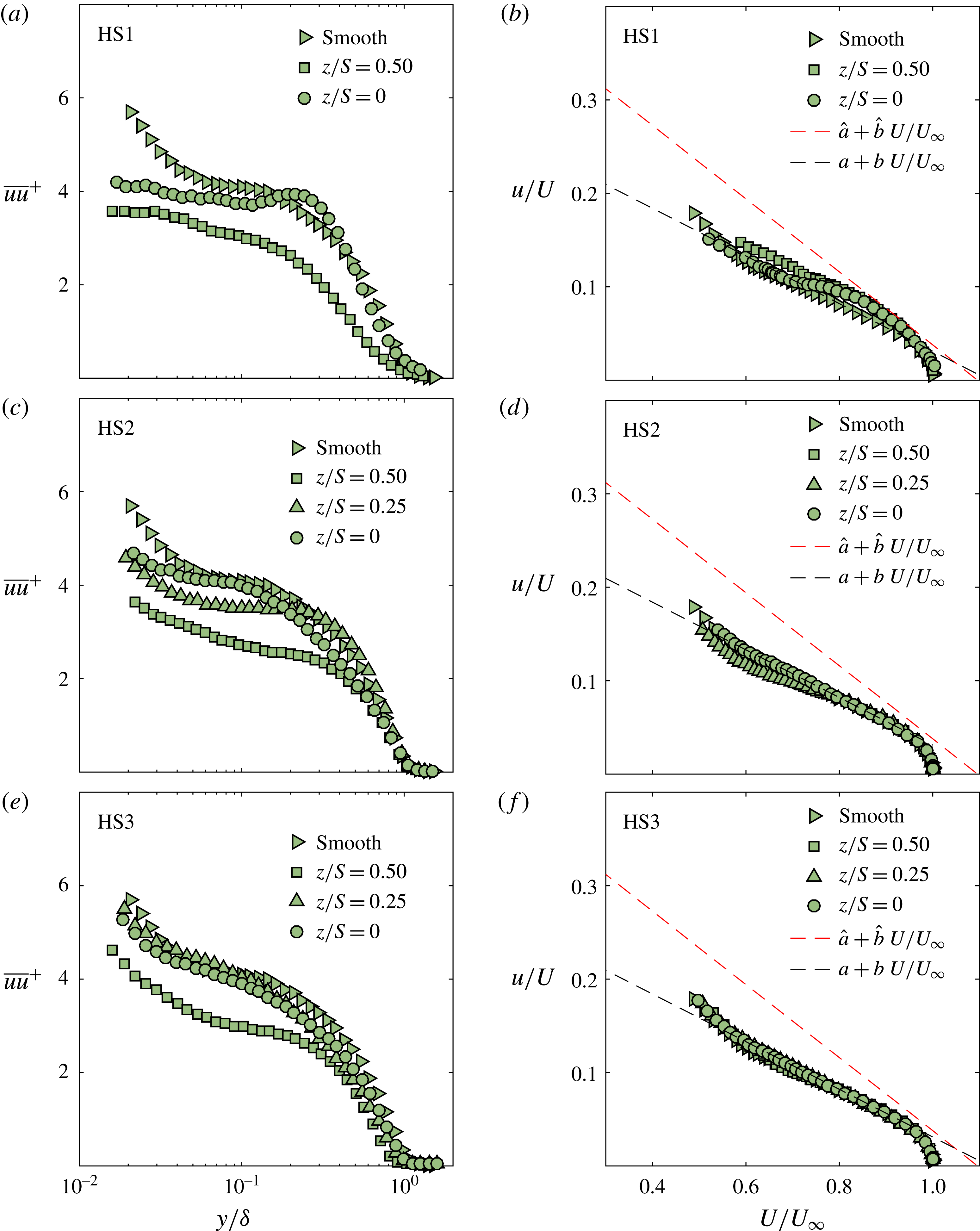
In order to assess the influence of these spanwise heterogeneous surfaces on turbulence statistics, inner-normalized turbulence intensity profiles are examined (figure 13
a,c,e). Variations in the normalized profiles between the measurements from different spanwise locations occur for each of the surfaces investigated. The differences in the magnitude along the span can be explained by the heterogeneity in spatial distribution of the wall shear stress. For instance, the value of
 $U_{\unicode[STIX]{x1D70F}}$
is locally higher at the peak and therefore normalizing the profiles with that value will lower the magnitude of turbulence compared to others. However, this alone cannot explain the lack of collapse since the shape of the profiles are substantially different. This would suggest the flow is influenced differently at different spanwise locations by the secondary motions. The lack of collapse of the normalized variance profiles is in line with results observed on the mean flow, which does not satisfy outer-layer similarity.
Effect of the surface heterogeneity on profiles of inner-normalized turbulence (a,c,e) and on the diagnostic plots (b,d,f) for the three spacings at
 $Re_{x}=3.9\times 10^{6}$
.

The lack of outer-layer similarity in both mean flow and turbulence could be further examined through the diagnostic plot, first introduced by Alfredsson, Segalini & Örlü (Reference Alfredsson, Segalini and Örlü2011). It plots the streamwise fluctuation normalized by the local mean streamwise velocity against local mean streamwise velocity normalized by the free stream velocity. This removes the dependence of the profiles on skin-friction velocity and helps reveal a region in the flow where the local turbulence intensity varies linearly with
 $U/U_{\infty }$
even in rough-wall flows, although the slope is different compared to smooth-wall flow but is independent of surface morphology for fully rough conditions (Castro, Segalini & Alfredsson Reference Castro, Segalini and Alfredsson2013). Although this might be the case for homogeneous surfaces, the cases where heterogeneity underpins the flow has not yet been considered. Figure 13 show the ‘diagnostic plots’ (b,d,f) for different spacings. The heterogeneity seems to have altered the profiles for HS1, where both the peak and valley profiles deviate from the smooth-wall and fully rough-wall slopes, exhibiting a non-canonical behaviour. This perhaps is due to the flow which is not fully rough. However, as the spacing increases (for HS2 and HS3), the data appear to collapse on the smooth-wall line. This means, locally, that despite the spanwise heterogeneities, the mean and turbulence go hand in hand. The relative motion of the turbulence and the mean flow structures are similar to those of a smooth wall, which seems to hold best for HS3 where the spacing is largest. This gives further evidence on the effect of secondary motions on the mean flow and turbulence. The secondary flow affects mean flow and turbulence in the outer region proportionally and therefore they tend to collapse in this diagnostic form. However, since the effect of secondary motion is not the same at the wall, this leads to lack of collapse when plotted in outer-layer similarity form.
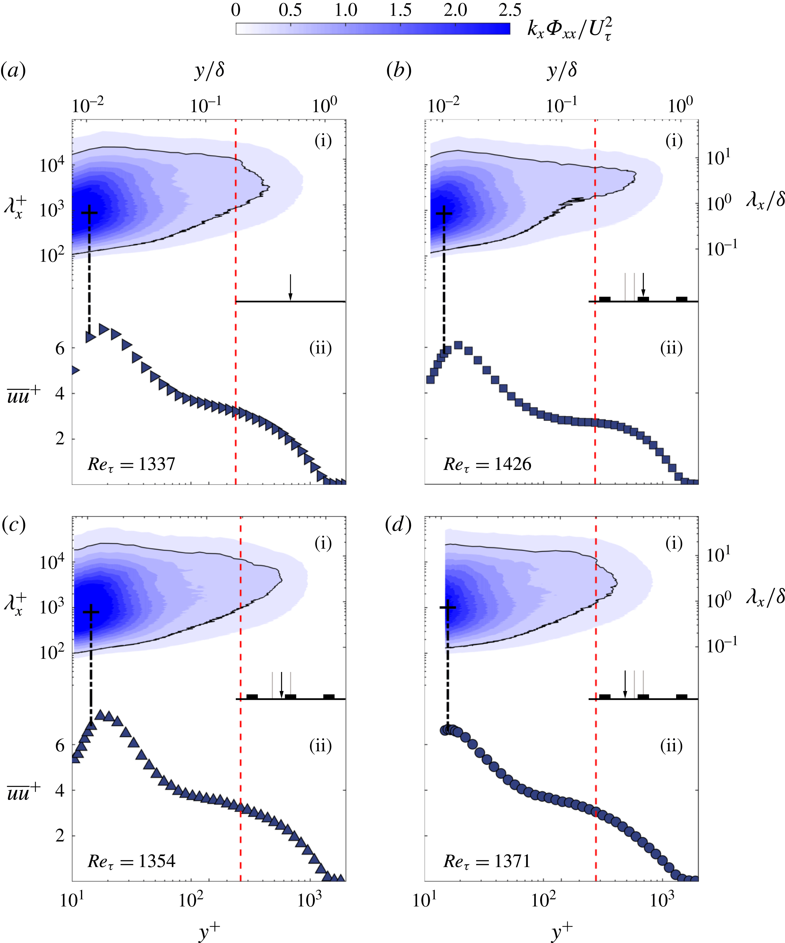
(i) Premultiplied streamwise energy spectrograms for the (a) smooth and (b–d) HS2 spacing case at
 $Re_{x}=2\times 10^{6}$
that are at relatively similar
 $Re_{\unicode[STIX]{x1D70F}}$
and (ii) their respective broadband turbulence intensities. The red-dashed line marks the edge of the inner/outer boundary layer while the black contour line represent the energy level at
 $k_{x}\unicode[STIX]{x1D6F7}_{xx}/U_{\unicode[STIX]{x1D70F}}^{2}=0.5$
.

In order to examine the scales that are affected by the spanwise heterogeneities, spectral analysis is performed. Figure 14 shows the inner-normalized premultiplied energy spectra of the streamwise velocity fluctuations against the inner-normalized wall distance
 $y^{+}$
together with the normalized turbulence profiles. A generic smooth-wall case as well as different spanwise locations from HS2 case are shown (at a low Reynolds number, where it is still possible to capture the near-wall peak for the HS2 case). The near-wall peak in turbulence as well as in the spectra is located at approximately
 $y^{+}\approx 15$
. The spectral peak is approximately at 1000 wall units. The existence of the peak is due to the presence of near-wall streaks in smooth walls. It seems that the spanwise heterogeneous smooth surface also retains the same characteristics at all spanwise locations. This further reinforces the claim that the effect of secondary flows on the near-wall region is limited and does not alter the structure or scaling locally in the viscous dominated region. Note that this behaviour cannot be captured at higher Reynolds number as the viscous sublayer becomes too small to be resolved in our measurements.
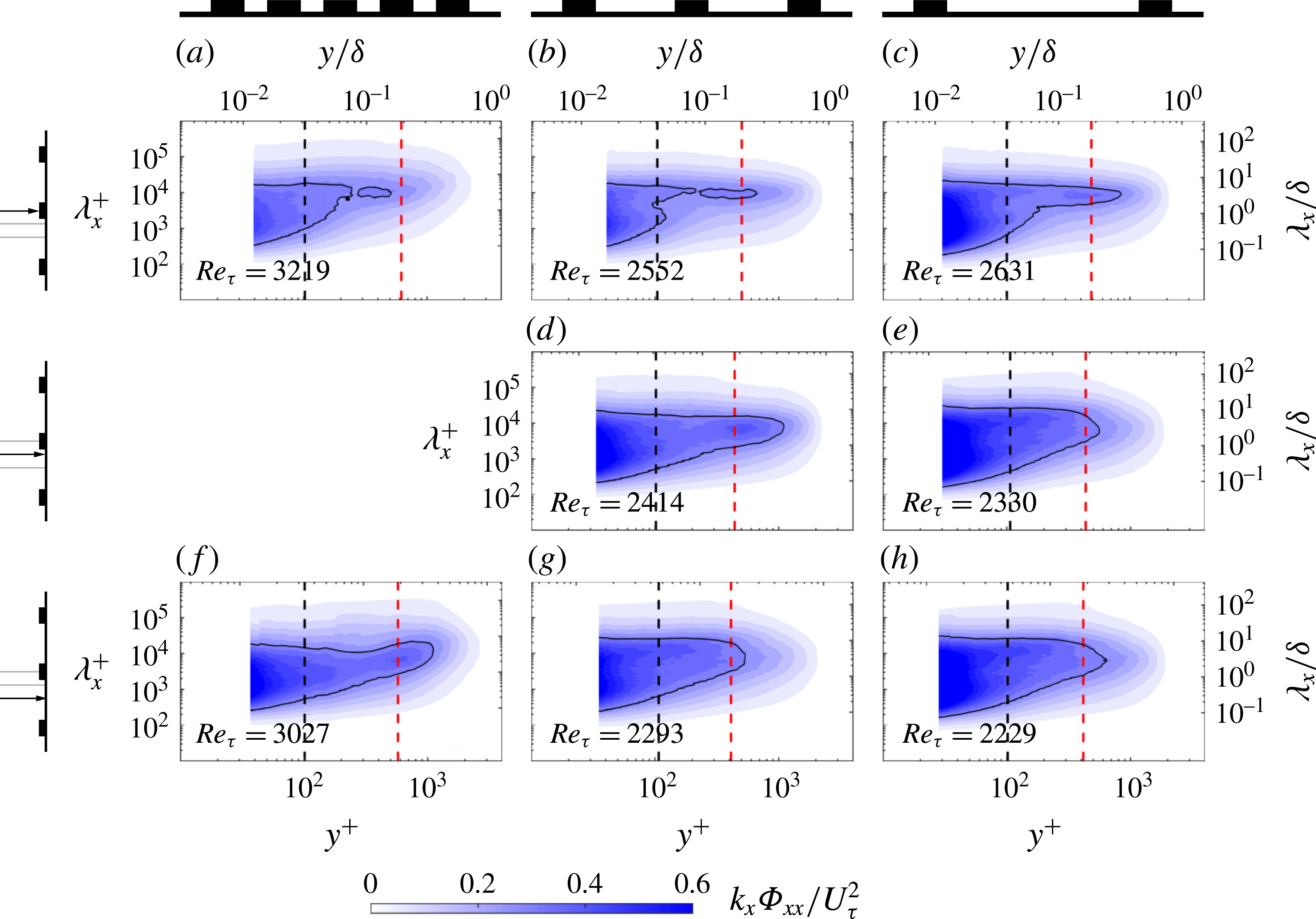
Premultiplied streamwise energy spectrograms for the three spacings at different spanwise locations at
 $Re_{x}=3.9\times 10^{6}$
. The columns are for different spacings and the rows are for different spanwise locations as indicated in the figure. The black-dashed lines mark the wall-normal location at
 $y^{+}\approx 100$
and the red-dashed lines at the wall-normal location
 $y/\unicode[STIX]{x1D6FF}\approx 0.2$
which are shown in figure 16 as extracted plots. The black contour lines represent the energy level at
 $k_{x}\unicode[STIX]{x1D6F7}_{xx}/U_{\unicode[STIX]{x1D70F}}^{2}=0.3$
.

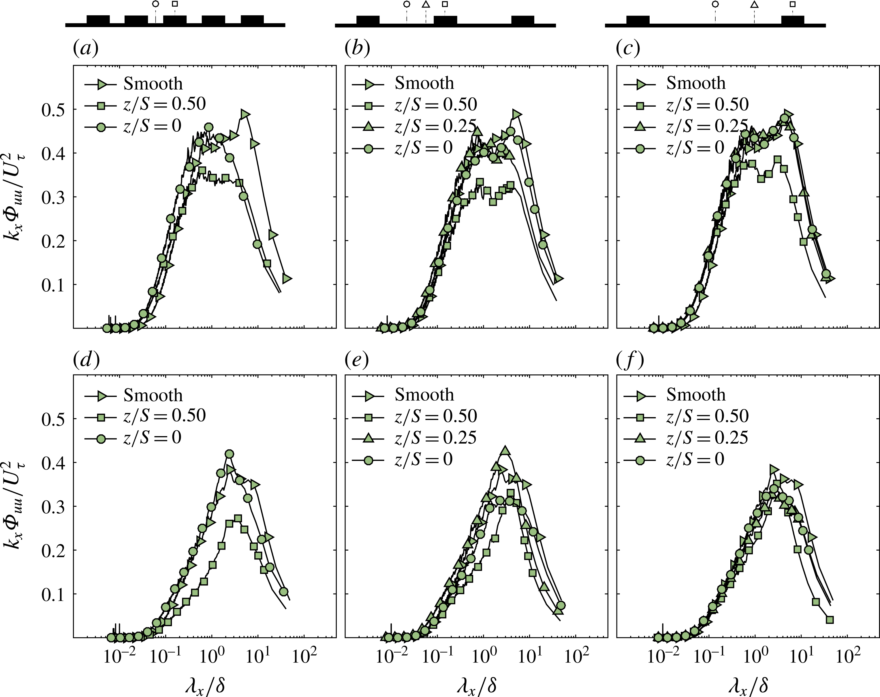
Normalized pre-multiplied energy spectra of the streamwise velocity fluctuation taken at
 $y^{+}\approx 100$
(a–c) and
 $y/\unicode[STIX]{x1D6FF}\approx 0.2$
(d–f) for the three spacings at
 $Re_{x}=3.9\times 10^{6}$
.

Spectrograms for the three different spacings (HS1, HS2 and HS3) at
 $Re_{x}\approx 4\times 10^{6}$
are shown in figure 15. The figure shows the spectrograms for each spacing in the columns and the spanwise locations of the measurement in the rows. Comparison of spectra at the peak (figure 15
a–c) across different spacings indicates that the spectra in the near-wall region become more energetic with increasing spacing. This is consistent with the variance profiles in the near-wall region. In fact, the near-wall energy content across all scales starts to approach that of a smooth wall with increasing spacing. However, at this location, the spectra will always be affected since the boundary layer is growing over an element of finite spanwise width and this will presumably generate secondary motions regardless of how large the spacing is between adjacent strips. In the outer region, this leads to a new energy containing region whose length scale is nearly constant with wall-normal location. The energy contained in this region increases with increasing spacing.
Figure 15(d,e) shows the premultiplied spectrograms at the mid-point between the peak and valley. This information is only available for HS2 and HS3 cases. HS3 appears to exhibits higher energy content compared to HS2 across all scales, especially in the inner region (i.e.
 $y^{+}<100$
). However, HS2 seems to indicate a local peak in the outer region, which is not observed in the case of HS3. This is presumably due to the fact that at this location (
 $z/S=0.25$
) the strength of the induced secondary motions that flank the surface elevation become weaker for a higher value of
 $S/\unicode[STIX]{x1D6FF}_{av}$
.
Figure 15(f–h) shows the variation in energy content at the valley of the three cases. The near-wall region of HS2 and HS3 appear to be similar for this spanwise location compared to HS1, which shows a less energetic near-wall region. However, in the outer region of HS1, an outer spectral peak seems to show as a higher energy content compared to the larger spacings is observed between
 $y/\unicode[STIX]{x1D6FF}=0.1$
and 0.3 for a range of wavelengths. Similar to the previous observation from (d,e) spectrograms, this also can be explained by the effect of the spacing between two adjacent strips.
In order to further assess the effect of surface heterogeneity on the spectra, a look at the energy distribution across the scales at two wall-normal locations for the three cases is presented. Figure 16 shows the premultiplied energy spectra at both
 $y^{+}\approx 100$
(figure 16
a–c) and
 $y/\unicode[STIX]{x1D6FF}\approx 0.2$
(figure 16
d–f) for different cases, which represent the black- and red-dashed lines in figure 15 respectively.
The energy distribution in the inner region (figure 16
a–c) reveals the presence of local similarity in the spectra. In fact, a degree of similarity seems to exist for the wavelengths smaller than
 $\unicode[STIX]{x1D706}_{x}\approx 0.3\unicode[STIX]{x1D6FF}$
across the spanwise locations, and increases with increasing spacing, whereas at wavelengths larger than
 $\unicode[STIX]{x1D706}_{x}\approx 0.3\unicode[STIX]{x1D6FF}$
, the collapse is essentially lost for the HS1 and HS2 cases. This indicates that in the inner region, the surface heterogeneity has a higher impact on the large scales than the small scales. The figure also shows that HS3 exhibits similarity with the smooth wall even at larger scales at
 $z/S=0.25$
and 0. This suggests that similarity (or collapse) is lost for
 $z/S=0.5$
while the presence of spectral similarity in the valley recovers (both at
 $z/S=0.25$
and 0) for higher values of
 $S/\unicode[STIX]{x1D6FF}_{av}$
. Therefore, there is a tendency to return to universality with increasing spacing. However, even for the largest spacing considered here (
 $S/\unicode[STIX]{x1D6FF}_{av}\approx 3.2$
), the large scales of the flow remain strongly affected by the surface heterogeneities at the surface elevation (
 $z/S=0.5$
). This is consistent with the very recent results presented by Yang & Anderson (Reference Yang and Anderson2018) who found that the features of spatial auto-correlations are strongly dependant on the length scale of the spanwise heterogeneity.
The energy distribution in the outer region (figure 16
d–f) reveals the existence of a similar trend for the small scales as in the inner region, where a good collapse in the small scales of the spectra (up to
 $\unicode[STIX]{x1D706}_{x}/\unicode[STIX]{x1D6FF}\approx 0.1$
) can be observed for all three cases across the different spanwise locations. Moreover, similarity seems to extend up to
 $\unicode[STIX]{x1D706}_{x}/\unicode[STIX]{x1D6FF}\approx 1$
for the valley profiles (both at
 $z/S=0.25$
and 0). Unlike the spectra at the valley, the premultiplied energy spectra at the surface elevation shows lack of similarity across all the scales for all three spacings. In fact, the magnitude of the outer spectral peak seems to be much lower compared to that of the valley regardless of the case. This effect tends to diminish with increasing spacing. This is in line with the findings of Nugroho et al. (Reference Nugroho, Hutchins and Monty2013), who made similar observations, where the overall magnitude of the energy spectra is lower than the smooth wall. This suggests that secondary motions induced by the heterogeneous surface start to add new energetic scales in the outer region, which will go towards negating the validity of outer-layer similarity. It should also be noted that
 $Re_{\unicode[STIX]{x1D70F}}$
decreases with increasing spacing and therefore the cases are not at matched friction Reynolds number (however, the variation is less than 20 % and is not going to significantly affect this observation.
At this stage, it is unclear which property (mean flow, turbulence statistics or the spectra) will return to similarity first with increasing spacing. Given that the secondary motions are sustained by turbulent transport, it is expected that these phenomena likely take place simultaneously. However, further studies are required to examine this in more detail.
5 Conclusions
The characteristics of a turbulent boundary layer under the influence of surface heterogeneities have been investigated. Idealized heterogeneous surfaces were created by means of smooth streamwise-aligned strips for three different spanwise spacings,
 $S/\unicode[STIX]{x1D6FF}_{av}\approx 0.8$
, 1.7 and 3.2. Previous studies suggest that these surfaces induce large-scale secondary motions (with decreasing strength/significance). Data for skin friction from OFI and single-point hot-wire velocity measurements were used to assess the limitations of similarity laws in these flows.
The effect of the surface heterogeneity on the wall drag was shown to both be a function of the spacing
 $S/\unicode[STIX]{x1D6FF}_{av}$
and Reynolds number indicating that the smooth heterogeneous surfaces were transitionally rough. The spanwise distribution of the
 $C_{f}$
was shown to have variations with surface heterogeneity. The ratio of the skin-friction coefficient at the peak and the valley of the surface was as high as 1.5 for HS1 (
 $S/\unicode[STIX]{x1D6FF}_{av}\approx 0.8$
) and down to 1.2 for HS3 (
 $S/\unicode[STIX]{x1D6FF}_{av}\approx 3.2$
). The spanwise-averaged skin friction was up to 30 % larger than a smooth wall and this value depends on the Reynolds number.
Mean velocity profiles at different spanwise locations exhibit a log layer and this was used to compute the roughness function and the zero-plane displacement. The zero-plane displacement was found to vary between 0.2
 $h$
and 0.7
 $h$
(
 $h$
is the height of the elevated smooth surface), however the measurements in the valley did not show any effective change in the location of the log layer. The roughness function however, was shown to vary along the spanwise direction with different regimes. This value of
 $\unicode[STIX]{x0394}U^{+}$
is consistent with those obtained from an integral method. As illustrated for HS2, at the surface elevation the skin friction is observed to constantly increase with
 $Re_{\unicode[STIX]{x1D703}}$
, however a transitional behaviour is observed at the valley, where
 $C_{f}$
is seen to decrease before increasing at the highest Reynolds number achieved in this experiment. The wake strength parameter
 $\unicode[STIX]{x1D6F1}$
was also assessed and was found to highly depend on the spanwise spacing. For
 $S/\unicode[STIX]{x1D6FF}_{av}\approx 0.8$
, the wake was completely cancelled and weaker than that of the smooth or rough-wall turbulent boundary layer. This can be related to the intermittency in the wake region which can be strongly affected by the presence of potential secondary flows, indicating a strong heterogeneity in the mean flow. The wake recovers at the valley to a smooth-wall value for higher spacings.
Mean velocity defect and turbulence intensity profiles do not follow outer-layer similarity across all locations for all cases. This suggests that even at the largest spacing of the study,
 $S/\unicode[STIX]{x1D6FF}_{av}\approx 3.2$
, the secondary motions essentially destroy similarity. However, the turbulence intensity appears to be universally related to the mean flow at all locations for HS2 and HS3, while HS1 showed the profiles to be lined between the smooth and rough linear fits examined through diagnostic plots. This suggests that beyond a certain spanwise spacing
 $S/\unicode[STIX]{x1D6FF}_{av}$
, the mean flow and turbulence possess a degree of local similarity to each other and do not reflect the conditions at the wall. This also suggests that the influence of the secondary flow at the wall is not of similar extent to that in the outer region. The deviation of outer-layer similarity appears to start recovering for larger spacing at the valley indicating that even a larger spacing is required to return to self-similarity.
The lack of similarity extends to spectra as well, with energy contained in the near-wall region increasing with increasing spacing (especially at the elevated surface), which is still less energetic than a smooth wall. However, for larger spacings, the spectra in the near-wall region appears to approach that of a smooth wall, especially for smaller wavelengths. The outer region starts to develop a new length scale (presumably from the secondary motions) across a range of wall positions for larger spacings. At the valley, an outer spectral peak is detected for
 $S/\unicode[STIX]{x1D6FF}_{av}\approx 0.8$
. The energy here is higher than that of a smooth wall but this peak is not apparent at larger spacings. The spectra in the outer region (beyond
 $y/\unicode[STIX]{x1D6FF}>0.2$
) appear to collapse in the smaller scales (
 $\unicode[STIX]{x1D706}_{x}<0.1\unicode[STIX]{x1D6FF}$
) across all spanwise positions with increasing spacing. This suggests that the effect of secondary motions is not necessarily felt at the smaller scales other than to reorganise their presence through turbulent transport.
Overall, this study has shown that the surface heterogeneity leads to a breakdown of outer-layer similarity in mean flow, turbulence statistics as well as spectra. Here we used an idealized heterogeneous surface with streamwise-oriented smooth ribs. This was done in order to directly measure the local skin friction, which was then used to assess the similarity. However, we believe that our findings should also be applicable to any heterogeneous rough/smooth surface where the characteristic spanwise length scale of the surface is comparable to the boundary-layer thickness resulting in secondary flows, regardless of the roughness height (e.g. Kevin et al.
Reference Kevin, Monty, Bai, Pathikonda, Nugroho, Barros, Christensen and Hutchins2017) or the roughness geometry (e.g. Barros & Christensen Reference Barros and Christensen2014, Anderson et al.
Reference Anderson, Barros, Christensen and Awasthi2015, Vanderwel & Ganapathisubramani Reference Vanderwel and Ganapathisubramani2015, Yang & Anderson Reference Yang and Anderson2018). The reason for lack of similarity can be attributed to the amplified radial motions due to local imbalances between the turbulence production and dissipation as postulated by Hinze (Reference Hinze1967, Reference Hinze1973) and more recently by Anderson et al. (Reference Anderson, Barros, Christensen and Awasthi2015), when
 $S/\unicode[STIX]{x1D6FF}_{av}\approx O(1)$
. This significantly changes the mean and the turbulent flow characteristics when compared to turbulent boundary layers over smooth or homogeneous rough walls, hence making the local skin friction inadequate to sufficiently satisfy outer-layer similarity. Further studies are required to identify how to appropriately scale the boundary-layer properties for flows over general heterogeneous surfaces.
Acknowledgements
The authors acknowledge the financial support of the European Research Council (ERC grant agreement no. 277472) and the Engineering and Physical Sciences Research Council of the United Kingdom (EPSRC grant ref. no. EP/L006383/1 and EP/P021476/1). C.V. is supported by a Marie-Curie fellowship (project ref no. 656081). T.M. is also partially support by the Faculty of Engineering and the Environment at the University of Southampton. The authors also thank the referees for their comments and suggestions. All data supporting this study are openly available from the University of Southampton repository at http://dx.doi.org/10.5258/SOTON/D0299.