1 Introduction
Fixed wing and flapping wing problems at high angle of attack (AoA) normally generate free vortices in the flow (Dickinson & Gotz Reference Dickinson and Gotz1993; Ellington et al. Reference Ellington, Van Den Berg, Willmott and Thomas1996; Wang Reference Wang2005; Muijres et al. Reference Muijres, Johansson, Barfield, Wolf, Spedding and Hedenstrom2008; Choudhry et al. Reference Choudhry, Leknys, Arjomandi and Kelso2014) and these free vortices may have significant impact on lift and drag (Polhamus Reference Polhamus1971; Wang Reference Wang2005; Choudhry et al. Reference Choudhry, Leknys, Arjomandi and Kelso2014). The free vortices may get attached to the body or move away from the body and enhance lift (Polhamus Reference Polhamus1971; Dickinson & Gotz Reference Dickinson and Gotz1993) or induce propulsion (Andersen et al. Reference Andersen, Bohr, Schnipper and Walther2017; Zhang Reference Zhang2017), depending on their position and velocity.
Vortex forces can be obtained in various ways – for instance by using the algebraic Bernoulli equation (Xia & Mohseni Reference Xia and Mohseni2013), the unsteady Blasius equation (Milne-Thomson Reference Milne-Thomson1960; Streitlien & Triantafyllou Reference Streitlien and Triantafyllou1995; Pitt Ford & Babinsky Reference Pitt Ford and Babinsky2013), or moment-equation-based integral approaches (Wu Reference Wu1981; Saffman Reference Saffman1992; Howe Reference Howe1995; Wu, Lu & Zhuang Reference Wu, Lu and Zhuang2007).
Known vortex force approaches require complete knowledge of the free vortex distribution at any instant. The free vortex distribution in the flow may be given by experimental visualization (Dickinson & Gotz Reference Dickinson and Gotz1993; Pitt Ford & Babinsky Reference Pitt Ford and Babinsky2013), discrete vortex simulation (Clement Reference Clement1973; Ansari, Zbikowski & Knowles Reference Ansari, Zbikowski and Knowles2006; Xia & Mohseni Reference Xia and Mohseni2013; Ramesh et al. Reference Ramesh, Gopalarathnam, Granlund, Ol and Edwards2014) and computational fluid dynamics (CFD) (Wang Reference Wang2000; Knowles et al. Reference Knowles, Wilkins, Ansari and Zbikowski2007; Li & Lu Reference Li and Lu2012). In special situations this distribution may be given by some analytical approach, including the concentrated vortex approach (Graham Reference Graham1983; Pullin & Wang Reference Pullin and Wang2004; Wang & Eldredge Reference Wang and Eldredge2012; Hemati, Eldredge & Speyer Reference Hemati, Eldredge and Speyer2014) and vortex sheet approaches (Wagner Reference Wagner1925; Graham Reference Graham1983; Jones Reference Jones2003; Pullin & Wang Reference Pullin and Wang2004). Graham, Pitt Ford & Babinsky (Reference Graham, Pitt Ford and Babinsky2017) derived a vortex force approach that requires an incomplete knowledge of the free vortex distribution.
Two issues remain to be further considered. The first is the lack of knowledge about critical regions in which a given vortex can be identified to enhance or reduce lift/drag. Li & Wu (Reference Li and Wu2015, Reference Li and Wu2016) proposed a vortex force map approach to identify whether a vortex is beneficial or harmful to the required force. The vortex force is expressed as the vector product of the vortex velocity and another vector called the vortex force factor. The vortex force factor depends only on the angle of attack and geometry. The vortex force factor is used to design vortex force lines. Depending on whether a vortex moves locally at an obtuse or an acute angle to the vortex force line, the force production or destruction effect of this vortex can be determined. With such an approach, a leading/trailing edge critical region for the leading/trailing edge vortex (LEV/TEV) to enhance or reduce lift are identified and these critical regions are amplified when the vortex follows a direction at a higher angle to the chord line. However, their studies were restricted to inviscid flow around a flat plate.
The second issue is the inconvenience of the usual vortex force approaches in treating vortices very far away from the body. The above vortex force methods are unsteady approaches by which the vortex force is related to the vortex velocity in such a way that even the starting vortex at infinity is considered to contribute lift. When applied to steady flow, the lift is associated with the starting vortex at infinity (Wu Reference Wu1981; Howe Reference Howe1995). This way is mathematically correct but is physically incompatible with the fact that only close-body vortices may induce pressure loads to cause lift. The steady approach usually associates the lift to the bound vortex and attached vortex. For instance, the classical Kutta–Joukowsky lift theorem relates the lift to the circulation of the bound vortex determined within the framework of the potential flow. When a vortex is attached to the airfoil, the enhanced lift is also related to the circulation of the attached vortex (Saffman & Sheffield Reference Saffman and Sheffield1977). A delta wing at high AoA uses an attached leading edge vortex to enhance lift; the pressure suction analogy of Polhamus (Reference Polhamus1971) relates the vortex force to this leading edge vortex. The pressure suction analogy has also been used to explain the lift-enhancing effect of an attached leading edge vortex of a flapping wing (Dickinson & Gotz Reference Dickinson and Gotz1993) and a trailing edge vortex (Li & Wu Reference Li and Wu2016) and to determine the vortex force of the attached leading edge vortex of insect wings (Traub Reference Traub2004; Ansari et al. Reference Ansari, Zbikowski and Knowles2006; Thielicke, Kesel & Stamhuis Reference Thielicke, Kesel and Stamhuis2011; Nabawy & Crowther Reference Nabawy and Crowther2014).
To overcome the drawbacks mentioned above, we propose in this paper to extend the vortex force map method of Li & Wu (Reference Li and Wu2016) for the normal force of a flat plate to viscous flows and general airfoils for both lift and drag, and to make a suitable vortex force decomposition in such a way that vortices far away enough from the body do not contribute to the force.
In § 2, the vortex force map approach of Li & Wu (Reference Li and Wu2016) for a flat plate is extended to arbitrary airfoils using Howe’s approach to determine the vortex force factors. A decomposed force formula is given, which ensures that the forces are sensitive only to near-body vortices. Then the way to build and apply new vortex force maps is provided. Li & Wu (Reference Li and Wu2016) considered vortex force maps only for the normal force; here we consider vortex force maps for both the normal force and the axial force, or lift and drag forces.
In § 3, the vortex force maps are displayed for various airfoils, including the Joukowsky airfoil and the NACA airfoil. The effect of airfoil thickness, camber and angle of attack will be discussed. The flow of the NACA0012 airfoil at a high angle of attack will be computed numerically and used to assess the vortex force method.
In appendix A, we outline the way to extend our approach to three dimensions.
2 Vortex force expression and vortex force maps for general airfoils
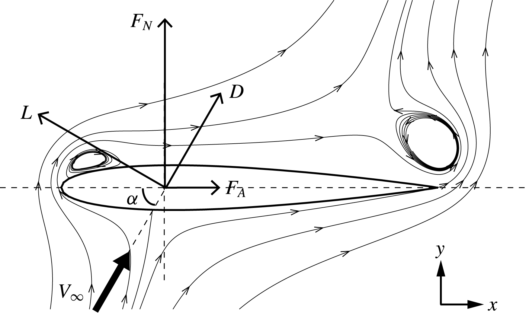
We consider viscous flows (inviscid flow is a special case) around a general airfoil at arbitrary AoA. Generally, there are free vortices attached or moving in such flows. Figure 1 is a schematic display of vortex flow around a general airfoil, in which the various force components are shown (
 $c_{A}$
is the chord length,
 $\unicode[STIX]{x1D6FC}$
is the angle of attack,
 $V_{\infty }$
, with
 $V_{\infty }>0$
, is the free-stream velocity in the body-fixed frame). The force vector has a normal component
 $F_{N}$
and an axial component
 $F_{A}$
, or a lift component
 $L$
and a drag component
 $D$
. The flow density
 $\unicode[STIX]{x1D70C}$
is constant since we only consider incompressible flow. The velocity of the flow is
 $\boldsymbol{U}=(u,v)$
and the vorticity is
 $\unicode[STIX]{x1D74E}$
. In two-dimensional flow there is only one component
 $\unicode[STIX]{x1D714}_{z}=(\unicode[STIX]{x2202}v/\unicode[STIX]{x2202}x)-(\unicode[STIX]{x2202}u/\unicode[STIX]{x2202}y)$
(spanwise component) for
 $\unicode[STIX]{x1D74E}$
. If a point or concentrated vortex is considered, its circulation is denoted
 $\unicode[STIX]{x1D6E4}$
(positive if it rotates in the counterclockwise direction). As in Li & Wu (Reference Li and Wu2016), the non-dimensional coordinate
 $$\begin{eqnarray}p={\displaystyle \frac{x-x_{m}}{{\textstyle \frac{1}{2}}c_{A}}},\quad q={\displaystyle \frac{y-y_{m}}{{\textstyle \frac{1}{2}}c_{A}}}\end{eqnarray}$$
will be used to display the vortex force map. Here,
 $(x_{m},y_{m})$
is the centre of the chord line of the airfoil.
Schematic display of vortex flow and various force components for a general airfoil at arbitrary angle of attack (
 $\unicode[STIX]{x1D6FC}$
) (
 $x$
is along the chord line and
 $y$
is perpendicular to the chord line). The force may be either decomposed into a normal component (
 $F_{N}$
) and an axial component (
 $F_{A}$
), or a lift component
 $(L)$
and a drag component (
 $D$
).

2.1 Standard vortex force method for general airfoils
The normal force for a flat plate due to any vortex of circulation
 $\unicode[STIX]{x1D6E4}$
was shown by Li & Wu (Reference Li and Wu2016) to be given by
 $$\begin{eqnarray}F_{N}=\unicode[STIX]{x1D70C}\unicode[STIX]{x1D726}_{N}\boldsymbol{\cdot }\boldsymbol{U}\unicode[STIX]{x1D6E4}.\end{eqnarray}$$
Here
 $\boldsymbol{U}=(u,v)$
is the vortex velocity in the body-fixed frame and
 $\unicode[STIX]{x1D726}_{N}=(P_{N},Q_{N})$
is the vector of vortex force factor. The vortex force factor also includes the image effect of the free vortex and is dependent only on the coordinate
 $(p,q)$
. For a flat plate,
 $$\begin{eqnarray}P_{N}(p,q)=1+2{\displaystyle \frac{\unicode[STIX]{x2202}E(p,q)}{\unicode[STIX]{x2202}p}}-{\displaystyle \frac{\unicode[STIX]{x2202}C(p,q)}{\unicode[STIX]{x2202}p}},\quad Q_{N}(p,q)=2{\displaystyle \frac{\unicode[STIX]{x2202}E(p,q)}{\unicode[STIX]{x2202}q}}-{\displaystyle \frac{\unicode[STIX]{x2202}C(p,q)}{\unicode[STIX]{x2202}q}},\end{eqnarray}$$
where
 $$\begin{eqnarray}\left.\begin{array}{@{}c@{}}C(p,q)={\displaystyle \frac{1}{\unicode[STIX]{x03C0}}}\left(p(\unicode[STIX]{x1D706}^{(0)}-\unicode[STIX]{x1D706}_{i}^{(1)})+\unicode[STIX]{x1D706}^{(1)}-{\displaystyle \frac{1}{2}}(\unicode[STIX]{x1D706}^{(0)}+\unicode[STIX]{x1D706}^{(2)})\right),\displaystyle \\ E(p,q)={\displaystyle \frac{1}{4\unicode[STIX]{x03C0}}}\left((p-1)(\unicode[STIX]{x1D706}^{(0)}+\unicode[STIX]{x1D706}^{(2)})+\left({\displaystyle \frac{3}{2}}-2p\right)\unicode[STIX]{x1D706}^{(1)}+{\displaystyle \frac{1}{2}}\unicode[STIX]{x1D706}^{(3)}\right),\end{array}\right\}\end{eqnarray}$$
and
 $$\begin{eqnarray}\unicode[STIX]{x1D706}^{(n)}=\int _{0}^{\unicode[STIX]{x03C0}}{\displaystyle \frac{\cos (n\unicode[STIX]{x1D6FD})}{(p+\cos \unicode[STIX]{x1D6FD})^{2}+q^{2}}}\,\text{d}\unicode[STIX]{x1D6FD},\quad n\geqslant 0\end{eqnarray}$$
is a geometrical parameter arising from the derivation of the vortex force.
Now we extend the vortex force approach to general airfoils, for both inviscid and viscous flows. Both normal force
 $F_{N}$
and axial force
 $F_{A}$
(these will be used to derive lift and drag in § 2.3, after stationary and moving vortex force decomposition presented in § 2.2) due to free vortices are considered.
Following (2.2), which is for the normal force due to a single vortex, the normal and axial force components for two-dimensional flow and due to all vortices for general airfoils and in viscous flow will also be expressed as
 $$\begin{eqnarray}F_{N}=\unicode[STIX]{x1D70C}\iint _{\unicode[STIX]{x1D6FA}}\boldsymbol{U}\boldsymbol{\cdot }\unicode[STIX]{x1D726}_{N}\unicode[STIX]{x1D714}_{z}\,\text{d}\unicode[STIX]{x1D6FA},\end{eqnarray}$$
and
 $$\begin{eqnarray}F_{A}=\unicode[STIX]{x1D70C}\iint _{\unicode[STIX]{x1D6FA}}\boldsymbol{U}\boldsymbol{\cdot }\unicode[STIX]{x1D726}_{A}\unicode[STIX]{x1D714}_{z}\,\text{d}\unicode[STIX]{x1D6FA}.\end{eqnarray}$$
Here
 $\unicode[STIX]{x1D726}_{N}$
and
 $\unicode[STIX]{x1D726}_{A}$
are vortex force factors, called standard vortex force factors here, for normal and axial forces. The integral is defined within the whole fluid region
 $\unicode[STIX]{x1D6FA}$
. Lift and drag formulae will be provided later on. The reason to have both a normal/axial force representation and a lift/drag representation in this paper is that vortex force map for normal/axial force representation is independent of the angle of attack, while the lift/drag representation is more convenient in application.
It is very difficult to use the same approach of Li & Wu (Reference Li and Wu2016) to obtain the vortex force vector
 $\unicode[STIX]{x1D726}_{N}$
and
 $\unicode[STIX]{x1D726}_{A}$
for general airfoils. Luckily, we find that the integral force theory of Howe (Reference Howe1995) can be used to do so. Note that Howe’s method was used by Lee et al. (Reference Lee, Hsieh, Chang and Chu2012) to study the vorticity forces on an impulsively started three-dimensional finite plate.
Howe (Reference Howe1995) derived the force expression of a rigid body due to free vortices in the body-fixed frame
 $$\begin{eqnarray}F_{k}=-\unicode[STIX]{x1D70C}\iiint _{\unicode[STIX]{x1D6FA}}\unicode[STIX]{x1D735}\unicode[STIX]{x1D719}_{k}\boldsymbol{\cdot }(\unicode[STIX]{x1D74E}\times \boldsymbol{U})\,\text{d}\unicode[STIX]{x1D6FA}.\end{eqnarray}$$
The formula (2.8) only gives the force due to free and image vortices. Forces due to skin friction and added mass effects (by acceleration, pitching and heaving of the body) are treated as independent force components by Howe (Reference Howe1995) and will not be considered in this paper. For flows with massive flow separation, recent studies showed that the forces are dominated by the vortex forces (Ansari et al. Reference Ansari, Zbikowski and Knowles2006; Xia & Mohseni Reference Xia and Mohseni2013; Li & Wu Reference Li and Wu2016) so in this paper we do not consider skin friction and added mass effects. Moreover, Howe (Reference Howe1995) also gave a similar formula for moment due to free vortices. In this paper we focus on the force, leaving the discussion of the moment for future works.
In (2.8),
 $\unicode[STIX]{x1D719}_{k}$
is the velocity potential of a hypothetical ideal fluid field induced by the translational motion of the body at unit speed in the
 $k\text{th}$
-direction. Expression (2.8) can then be used to give the normal force
 $F_{N}$
and axial force
 $F_{A}$
in the form of (2.6) and (2.7), with the standard vortex force factors given by
 $$\begin{eqnarray}\unicode[STIX]{x1D726}_{N}=(P_{N},Q_{N})=\left({\displaystyle \frac{\unicode[STIX]{x2202}\unicode[STIX]{x1D719}_{N}}{\unicode[STIX]{x2202}y}},-{\displaystyle \frac{\unicode[STIX]{x2202}\unicode[STIX]{x1D719}_{N}}{\unicode[STIX]{x2202}x}}\right),\end{eqnarray}$$
and
 $$\begin{eqnarray}\unicode[STIX]{x1D726}_{A}=(P_{A},Q_{A})=\left({\displaystyle \frac{\unicode[STIX]{x2202}\unicode[STIX]{x1D719}_{A}}{\unicode[STIX]{x2202}y}},-{\displaystyle \frac{\unicode[STIX]{x2202}\unicode[STIX]{x1D719}_{A}}{\unicode[STIX]{x2202}x}}\right).\end{eqnarray}$$
Now, for the body-fixed frame,
 $\unicode[STIX]{x1D719}_{N}$
and
 $\unicode[STIX]{x1D719}_{A}$
are the hypothetical potentials for a fixed body with unitary inflow from infinity, i.e.
 $$\begin{eqnarray}\left.\begin{array}{@{}c@{}}{\displaystyle \frac{\unicode[STIX]{x2202}^{2}\unicode[STIX]{x1D719}_{N}}{\unicode[STIX]{x2202}x^{2}}}+{\displaystyle \frac{\unicode[STIX]{x2202}^{2}\unicode[STIX]{x1D719}_{N}}{\unicode[STIX]{x2202}y^{2}}}=0,\displaystyle \\ {\displaystyle \frac{\unicode[STIX]{x2202}\unicode[STIX]{x1D719}_{N}}{\unicode[STIX]{x2202}n}}=0\quad (x,y)\rightarrow S_{B},\\ {\displaystyle \frac{\unicode[STIX]{x2202}\unicode[STIX]{x1D719}_{N}}{\unicode[STIX]{x2202}y}}=-1,\quad {\displaystyle \frac{\unicode[STIX]{x2202}\unicode[STIX]{x1D719}_{N}}{\unicode[STIX]{x2202}x}}=0\quad (x,y)\rightarrow \infty ,\end{array}\right\}\end{eqnarray}$$
 $$\begin{eqnarray}\left.\begin{array}{@{}c@{}}{\displaystyle \frac{\unicode[STIX]{x2202}^{2}\unicode[STIX]{x1D719}_{A}}{\unicode[STIX]{x2202}x^{2}}}+{\displaystyle \frac{\unicode[STIX]{x2202}^{2}\unicode[STIX]{x1D719}_{A}}{\unicode[STIX]{x2202}y^{2}}}=0,\displaystyle \\ {\displaystyle \frac{\unicode[STIX]{x2202}\unicode[STIX]{x1D719}_{A}}{\unicode[STIX]{x2202}n}}=0\quad (x,y)\rightarrow S_{B},\displaystyle \\ {\displaystyle \frac{\unicode[STIX]{x2202}\unicode[STIX]{x1D719}_{A}}{\unicode[STIX]{x2202}y}}=0,\quad {\displaystyle \frac{\unicode[STIX]{x2202}\unicode[STIX]{x1D719}_{A}}{\unicode[STIX]{x2202}x}}=-1\quad (x,y)\rightarrow \infty .\end{array}\right\}\end{eqnarray}$$
Here,
 $S_{B}$
denotes the body surface. Thus, to obtain the vortex force factors
 $\unicode[STIX]{x1D726}_{N}$
and
 $\unicode[STIX]{x1D726}_{A}$
, one simply needs to solve the Laplace models (2.11) and (2.12). For three-dimensional flow, three Laplace models should be solved (appendix A).
With the normal and axial force components given by (2.18) and (2.20), the lift
 $L$
and drag
 $D$
, for AoA equal to
 $\unicode[STIX]{x1D6FC}$
, are obtained as
 $$\begin{eqnarray}\left.\begin{array}{@{}c@{}}L=F_{N}\cos \unicode[STIX]{x1D6FC}-F_{A}\sin \unicode[STIX]{x1D6FC},\\ D=F_{N}\sin \unicode[STIX]{x1D6FC}+F_{A}\cos \unicode[STIX]{x1D6FC}.\end{array}\right\}\end{eqnarray}$$
If (2.6) and (2.7) are used, then we obtain the standard vortex lift and drag force formulae for general airfoils
 $$\begin{eqnarray}\left.\begin{array}{@{}c@{}}L=\unicode[STIX]{x1D70C}\displaystyle \iint _{\unicode[STIX]{x1D6FA}}\boldsymbol{U}\boldsymbol{\cdot }\unicode[STIX]{x1D726}_{L}\unicode[STIX]{x1D714}_{z}\,\text{d}\unicode[STIX]{x1D6FA},\displaystyle \\ D=\unicode[STIX]{x1D70C}\displaystyle \iint _{\unicode[STIX]{x1D6FA}}\boldsymbol{U}\boldsymbol{\cdot }\unicode[STIX]{x1D726}_{D}\unicode[STIX]{x1D714}_{z}\,\text{d}\unicode[STIX]{x1D6FA},\end{array}\right\}\end{eqnarray}$$
where
 $$\begin{eqnarray}\left.\begin{array}{@{}c@{}}\unicode[STIX]{x1D726}_{L}=\unicode[STIX]{x1D726}_{N}\cos \unicode[STIX]{x1D6FC}-\unicode[STIX]{x1D726}_{A}\sin \unicode[STIX]{x1D6FC},\displaystyle \\ \unicode[STIX]{x1D726}_{D}=\unicode[STIX]{x1D726}_{N}\sin \unicode[STIX]{x1D6FC}+\unicode[STIX]{x1D726}_{A}\cos \unicode[STIX]{x1D6FC},\end{array}\right\}\end{eqnarray}$$
are standard vortex lift and drag factors.
2.2 Decomposed vortex force expressions avoiding far-away vortices having non-negligible force effect
Physically, only near-body vortices are more likely to cause pressure variation, while vortices far away from the body have negligible effects on the force. However, in traditional unsteady vortex force approaches, including the one presented in § 2.1, far-away vortices (including starting vortices at infinity, see for instance Wu (Reference Wu1981) and Howe (Reference Howe1995)) also have important effects on the force. This is inconvenient in those applications where far-away vortices cannot be captured in a proper way (far-away vortices are difficult to measure experimentally and are not computed in computational fluid dynamics based on a truncated domain).
Here we propose to decompose the force expressions into several terms in such a way that only near-body vortices have important effects. To achieve this purpose, we first rewrite the force expressions on the ground-fixed frame. Li & Wu (Reference Li and Wu2016) have already suggested a method to rewrite (2.2) on the ground-fixed frame. Now we follow Li & Wu (Reference Li and Wu2016) to rewrite both (2.6) and (2.7) on the ground-fixed frame, by defining
 $$\begin{eqnarray}\overline{u}=u-V_{\infty }^{(h)},\quad \overline{v}=v-V_{\infty }^{(v)},\quad \overline{\boldsymbol{U}}=(\overline{u},\overline{v}).\end{eqnarray}$$
Here
 $V_{\infty }^{(h)}=V_{\infty }\cos \unicode[STIX]{x1D6FC}$
,
 $V_{\infty }^{(v)}=V_{\infty }\sin \unicode[STIX]{x1D6FC}$
and
 $\overline{\boldsymbol{U}}$
is the velocity relative to the ground frame. A starting vortex at infinity (relative to the body) has vanishing
 $\overline{\boldsymbol{U}}$
on the ground-fixed frame.
Assuming that
 $\unicode[STIX]{x1D6E4}_{b}$
is the bound circulation (which vanishes for the viscous flow model but has a finite magnitude for the inviscid flow model). Then, by Kelvin’s vorticity conservation theorem, we have
 $$\begin{eqnarray}\unicode[STIX]{x1D6E4}_{b}+\iint _{\unicode[STIX]{x1D6FA}}\unicode[STIX]{x1D714}_{z}\,\text{d}\unicode[STIX]{x1D6FA}=0.\end{eqnarray}$$
Adding
 $-\unicode[STIX]{x1D70C}(\unicode[STIX]{x1D6E4}_{b}+\iint _{\unicode[STIX]{x1D6FA}}\unicode[STIX]{x1D714}_{z}\,\text{d}\unicode[STIX]{x1D6FA})V_{\infty }^{(h)}$
to the normal force formula (2.6) and substituting (2.16) in it gives the normal force as the sum of three components
 $$\begin{eqnarray}\left.\begin{array}{@{}c@{}}\displaystyle F_{N}=F_{N}^{(B)}+F_{N}^{(1)}+F_{N}^{(2)},\\ \displaystyle F_{N}^{(B)}=-\unicode[STIX]{x1D70C}V_{\infty }^{(h)}\unicode[STIX]{x1D6E4}_{b},\\ F_{N}^{(1)}=\displaystyle \iint _{\unicode[STIX]{x1D6FA}}\unicode[STIX]{x1D70C}\unicode[STIX]{x1D726}_{N}\boldsymbol{\cdot }\overline{\boldsymbol{U}}\unicode[STIX]{x1D714}_{z}\,\text{d}\unicode[STIX]{x1D6FA},\\ \displaystyle F_{N}^{(2)}=\displaystyle \iint _{\unicode[STIX]{x1D6FA}}\unicode[STIX]{x1D70C}\boldsymbol{K}_{N}\boldsymbol{\cdot }\boldsymbol{V}_{\infty }\unicode[STIX]{x1D714}_{z}\,\text{d}\unicode[STIX]{x1D6FA}.\end{array}\right\}\end{eqnarray}$$
Here,
 $F_{N}^{(B)}$
is the bound vortex force,
 $F_{N}^{(1)}$
depends on the free-stream velocity while
 $F_{N}^{(2)}$
depends on the local velocity. The expressions for
 $\boldsymbol{K}_{N}$
and
 $\unicode[STIX]{x1D726}_{N}$
are
 $$\begin{eqnarray}\left.\begin{array}{@{}c@{}}\unicode[STIX]{x1D726}_{N}(p,q)=(P_{N}(p,q),Q_{N}(p,q)),\displaystyle \\ \boldsymbol{K}_{N}(p,q)=(P_{N}(p,q)-1,Q_{N}(p,q)).\end{array}\right\}\end{eqnarray}$$
Similarly, adding
 $\unicode[STIX]{x1D70C}(\unicode[STIX]{x1D6E4}_{b}+\iint _{\unicode[STIX]{x1D6FA}}\unicode[STIX]{x1D714}_{z}\,\text{d}\unicode[STIX]{x1D6FA})V_{\infty }^{(v)}$
to the axial force formula (2.7) and substituting (2.16) in it gives
 $$\begin{eqnarray}\left.\begin{array}{@{}c@{}}F_{A}=F_{A}^{(B)}+F_{A}^{(1)}+F_{A}^{(2)},\displaystyle \\ F_{A}^{(B)}=\unicode[STIX]{x1D70C}V_{\infty }^{(v)}\unicode[STIX]{x1D6E4}_{b},\displaystyle \\ F_{A}^{(1)}=\displaystyle \iint _{\unicode[STIX]{x1D6FA}}\unicode[STIX]{x1D70C}\unicode[STIX]{x1D726}_{A}\boldsymbol{\cdot }\overline{\boldsymbol{U}}\unicode[STIX]{x1D714}_{z}\,\text{d}\unicode[STIX]{x1D6FA},\\ F_{A}^{(2)}=\displaystyle \iint _{\unicode[STIX]{x1D6FA}}\unicode[STIX]{x1D70C}\boldsymbol{K}_{A}\boldsymbol{\cdot }\boldsymbol{V}_{\infty }\unicode[STIX]{x1D714}_{z}\,\text{d}\unicode[STIX]{x1D6FA},\end{array}\right\}\end{eqnarray}$$
with
 $$\begin{eqnarray}\left.\begin{array}{@{}c@{}}\unicode[STIX]{x1D726}_{A}(p,q)=(P_{A}(p,q),Q_{A}(p,q)),\displaystyle \\ \boldsymbol{K}_{A}(p,q)=(P_{A}(p,q),Q_{A}(p,q)+1).\end{array}\right\}\end{eqnarray}$$
Now we discuss the meaning of the decomposed force formulae.
(i) The first terms
 $F_{N}^{(B)}$
,
 $F_{A}^{(B)}$
are the force components of Joukowsky type due to the bound vortex
 $\unicode[STIX]{x1D6E4}_{b}$
for the inviscid flow model (which vanishes for the viscous flow model). In steady inviscid flow without any free vortex, these are the sole force contributions.
(ii) The second terms
 $F_{N}^{(1)},F_{A}^{(1)}$
are the vortex forces depending on the local velocity
 $\overline{\boldsymbol{U}}=(\overline{u},\overline{v})$
. Since
 $\overline{\boldsymbol{U}}$
is defined on a ground-fixed frame, a vortex far away from the body has
 $\overline{\boldsymbol{U}}\rightarrow 0$
. This means that a vortex far away enough from the body does not contribute to force by this component.
(iii) The third terms
 $F_{N}^{(2)},F_{A}^{(2)}$
are the vortex force components depending on the free-stream velocity. Note that
 $P_{N}=1$
,
 $Q_{N}=0$
and
 $P_{A}=0$
,
 $Q_{A}=-1$
and thus
 $\boldsymbol{K}_{N}=\boldsymbol{K}_{A}=0$
for any vortex that is very far away from the airfoil. Thus a vortex far away enough from the body does not contribute to these components.
(iv) Since vortices very far away from the body contribute to none of the components, the decomposed vortex force approach is compatible with the physics that only near-body vortices induce a pressure load on the body to affect forces.
Now consider the force formulae for lift and drag. Putting (2.18) and (2.20) into (2.13) gives the decomposed vortex lift formula
 $$\begin{eqnarray}\left.\begin{array}{@{}c@{}}L=L^{(B)}+L^{(1)}+L^{(2)},\displaystyle \\ L^{(B)}=-\unicode[STIX]{x1D70C}V_{\infty }\unicode[STIX]{x1D6E4}_{b},\displaystyle \\ L^{(1)}=\displaystyle \iint _{\unicode[STIX]{x1D6FA}}\unicode[STIX]{x1D70C}\unicode[STIX]{x1D726}_{L}\boldsymbol{\cdot }\overline{\boldsymbol{U}}\unicode[STIX]{x1D714}_{z}\,\text{d}\unicode[STIX]{x1D6FA},\displaystyle \\ L^{(2)}=\displaystyle \iint _{\unicode[STIX]{x1D6FA}}\unicode[STIX]{x1D70C}\boldsymbol{K}_{L}\boldsymbol{\cdot }\boldsymbol{V}_{\infty }\unicode[STIX]{x1D714}_{z}\,\text{d}\unicode[STIX]{x1D6FA},\end{array}\right\}\end{eqnarray}$$
and vortex drag formula
 $$\begin{eqnarray}\left.\begin{array}{@{}c@{}}D=D^{(B)}+D^{(1)}+D^{(2)},\displaystyle \\ D^{(B)}=0,\\ D^{(1)}=\displaystyle \iint _{\unicode[STIX]{x1D6FA}}\unicode[STIX]{x1D70C}\unicode[STIX]{x1D726}_{D}\boldsymbol{\cdot }\overline{\boldsymbol{U}}\unicode[STIX]{x1D714}_{z}\,\text{d}\unicode[STIX]{x1D6FA},\displaystyle \\ D^{(2)}=\displaystyle \iint _{\unicode[STIX]{x1D6FA}}\unicode[STIX]{x1D70C}\boldsymbol{K}_{D}\boldsymbol{\cdot }\boldsymbol{V}_{\infty }\unicode[STIX]{x1D714}_{z}\,\text{d}\unicode[STIX]{x1D6FA},\end{array}\right\}\end{eqnarray}$$
where
 $$\begin{eqnarray}\left.\begin{array}{@{}c@{}}\unicode[STIX]{x1D726}_{L}(p,q)=\unicode[STIX]{x1D726}_{N}(p,q)\cos \unicode[STIX]{x1D6FC}-\unicode[STIX]{x1D726}_{A}(p,q)\sin \unicode[STIX]{x1D6FC},\\ \boldsymbol{K}_{L}(p,q)=\boldsymbol{K}_{N}(p,q)\cos \unicode[STIX]{x1D6FC}-\boldsymbol{K}_{A}(p,q)\sin \unicode[STIX]{x1D6FC},\end{array}\right\}\end{eqnarray}$$
and
 $$\begin{eqnarray}\left.\begin{array}{@{}c@{}}\unicode[STIX]{x1D726}_{D}(p_{i},q_{i})=\unicode[STIX]{x1D726}_{N}(p,q)\sin \unicode[STIX]{x1D6FC}+\unicode[STIX]{x1D726}_{A}(p,q)\cos \unicode[STIX]{x1D6FC},\\ \boldsymbol{K}_{D}(p,q)=\boldsymbol{K}_{N}(p,q)\sin \unicode[STIX]{x1D6FC}+\boldsymbol{K}_{A}(p,q)\cos \unicode[STIX]{x1D6FC}.\end{array}\right\}\end{eqnarray}$$
2.3 Vortex force map and method to apply the vortex force method
As in Li & Wu (Reference Li and Wu2016), the vortex force method is useful to design vortex force maps for identifying favourable directions and critical regions for force production/destruction of a given vortex. The vortex force map approach can also be used to obtain the vortex force if the properties of vortices (velocity and circulation) in the flow are obtained by some analytical, numerical or experimental methods.
(i) Force map analysis
Following and extending the work of Li & Wu (Reference Li and Wu2016), here the vortex force map in the two-dimensional plane
 $(p,q)$
contains force lines that are locally parallel to the vortex force vector (
 $\unicode[STIX]{x1D726}_{N}$
for normal force and
 $\unicode[STIX]{x1D726}_{A}$
for axial force, with
 $\unicode[STIX]{x1D726}_{N}$
and
 $\unicode[STIX]{x1D726}_{A}$
given by (2.9) and (2.10), and
 $\unicode[STIX]{x1D726}_{L}$
for lift force and
 $\unicode[STIX]{x1D726}_{D}$
for drag force, with
 $\unicode[STIX]{x1D726}_{L},\unicode[STIX]{x1D726}_{D}$
given by (2.15)).
Force lines are parallel to the vortex force vector in the same way as streamlines are locally parallel to the fluid velocity. Vortex force lines can thus be obtained through a streamline designer, with the velocity replaced by the vortex force factors. Force lines are independent of the specific flow conditions. The vortex force of any freely moving vortex thus depends on the angle between the vortex force line and the streamline at the point of the vortex. By examining the local direction of the force line and the magnitude of the scalar vortex force factor
 $\unicode[STIX]{x1D6EC}_{N},\unicode[STIX]{x1D6EC}_{A},\unicode[STIX]{x1D6EC}_{L}$
or
 $\unicode[STIX]{x1D6EC}_{D}$
(which can also be displayed as contour lines), it is easy to identify the force contribution effect of any given vortex in the flow, in the sense that any individual vortex is interpreted to have a force. The force increasing/decreasing effect of a given vortex can thus be identified according to its circulation (sign and magnitude), position and direction, in the same way as for normal force studied by Li & Wu (Reference Li and Wu2016). Two types of vortices, with different circulation signs, should be considered since the vortex force depends on the sign of the circulation. An LEV (which may also denote a leading edge vortex since such a vortex usually has
 $\unicode[STIX]{x1D6E4}<0$
) denotes a vortex having a circulation
 $\unicode[STIX]{x1D6E4}<0$
(i.e. rotating in the clockwise direction) while a TEV (which may denote a trailing edge vortex for the same reason) denotes a vortex having
 $\unicode[STIX]{x1D6E4}>0.$
For the normal force of a flat plate, Li & Wu (Reference Li and Wu2016) used the vortex force map analysis to identify favourable directions and critical regions for force production/destruction of a given vortex. For instance, there is a closed critical region just above the leading edge where leading edge vortices enhance the normal force and another one above the trailing edge where trailing edge vortices enhance the normal force. This means that both leading edge and trailing edge vortices may enhance the normal force provided they are somewhere above the airfoil to efficiently cause pressure suction. We are wondering here whether the vortex force lines for general airfoils are similar to the flat plate case. If so, then the conclusion of existence of critical regions for a flat plate also holds true for general airfoils.
(ii) Vortex force analysis
The vortex force factors can be precomputed for a given airfoil, then force can be directly obtained from the vortex force formulae once
 $\boldsymbol{U}$
and
 $\unicode[STIX]{x1D714}_{z}$
are computed or measured. This can be done as follows.
Given the geometry of the airfoil, we solve (2.11)–(2.12) to get
 $\unicode[STIX]{x1D719}_{N}$
and
 $\unicode[STIX]{x1D719}_{A}$
, these
 $\unicode[STIX]{x1D719}_{N}$
and
 $\unicode[STIX]{x1D719}_{A}$
are put into (2.9) and (2.10) to get the vortex force factors
 $(P_{N},Q_{N})$
and
 $(P_{A},Q_{A})$
. These factors depend only on the geometry (shape of the airfoil) and are independent of other conditions such as angle of attack and Reynolds number. The flow vorticity
 $\unicode[STIX]{x1D714}_{z}$
and velocity
 $\boldsymbol{U}$
may be obtained by some conventional methods (discrete vortex simulation, computational fluid dynamics simulation, experimental measurement).
(i) If the standard force approach is used, put
 $(P_{N},Q_{N})$
and
 $(P_{A},Q_{A})$
into (2.9) and (2.10) to get
 $\unicode[STIX]{x1D726}_{N}$
and
 $\unicode[STIX]{x1D726}_{A}$
, then use (2.6) and (2.7) to get the normal and axial forces. If lift and drag are to be obtained for a given angle of attack, then (2.13) is used.
(ii) If the decomposed force approach is to be used, then put
 $(P_{N},Q_{N})$
and
 $(P_{A},Q_{A})$
into (2.19) and (2.21) to get the vortex force factors
 $\boldsymbol{K}_{N}$
,
 $\boldsymbol{K}_{A}$
,
 $\unicode[STIX]{x1D726}_{N}$
and
 $\unicode[STIX]{x1D726}_{A}$
and use (2.18) and (2.20) to get normal and axial forces. Finally, (2.22) and (2.23) are used to get the lift and drag.
For simple airfoils like flat plates and Joukowsky airfoils, equations (2.11) and (2.12) have analytical solutions, but for more general airfoils, we should use numerical methods to solve these equations to get
 $\unicode[STIX]{x1D719}_{N}$
and
 $\unicode[STIX]{x1D719}_{A}$
. More details will be given in the next section.
3 Vortex force study for specific airfoils
In this section, the Joukowsky airfoil and the NACA0012 airfoil are used to demonstrate how to build the vortex force map and identify the effect of given vortices. For the Joukowsky airfoil the effects of thickness, camber and angle of attack on the vortex force map are considered. For the NACA0012 airfoil, the vortex force maps for different AoAs are displayed and the vortex force approach is verified against CFD results for different AoAs and for different Reynolds numbers. This study permits us to understand the sensitivity of vortex force maps to the airfoil geometry and to know whether the vortex force behaviour observed for a flat plate (Li & Wu Reference Li and Wu2016) still exists for general airfoils. Moreover, this study allows us to validate the vortex force approach. Both the standard force formulae defined by (2.14) and the decomposed force formulae defined by (2.22)–(2.23) will be considered.
3.1 Application to Joukowsky airfoil, effects of airfoil geometry and angle of attack
For a Joukowsky airfoil with a given thickness
 $b$
, a camber
 $f$
, and chord length
 $c_{A}=4a$
, the solutions
 $\unicode[STIX]{x1D719}_{N}$
and
 $\unicode[STIX]{x1D719}_{A}$
of (2.11) and (2.12) can be obtained analytically through conformal mapping and these solutions can further be used to obtain the analytical formulae for the vortex force factors
 $\unicode[STIX]{x1D726}_{N}$
and
 $\unicode[STIX]{x1D726}_{A}$
through (2.9) and (2.10). The numerical method used in § 3.2 to solve the Laplace models (2.11) and (2.12) for
 $\unicode[STIX]{x1D719}_{N}$
and
 $\unicode[STIX]{x1D719}_{A}$
is also tried here, giving the same result as the analytical method.
3.1.1 Analytical solution for vortex force factors
Let
 $\text{i}=\sqrt{-1}$
, we use
 $\unicode[STIX]{x1D701}=\unicode[STIX]{x1D709}+\text{i}\unicode[STIX]{x1D702}$
to denote a point in the circle plane and
 $z=x+\text{i}y$
to denote a point in the physical plane. The coordinates of both planes are related by the Joukowsky transformation
 $z=\unicode[STIX]{x1D701}+a^{2}/\unicode[STIX]{x1D701}$
. The solutions
 $\unicode[STIX]{x1D719}_{N}$
and
 $\unicode[STIX]{x1D719}_{A}$
of (2.11) and (2.12) in the circle plane can be easily constructed and then mapped into the physical plane to give
 $$\begin{eqnarray}\unicode[STIX]{x1D719}_{N}=\text{Im}\left[(f(z)-\unicode[STIX]{x1D701}_{c})-{\displaystyle \frac{c^{2}}{(f(z)-\unicode[STIX]{x1D701}_{c})}}\right],\quad \unicode[STIX]{x1D719}_{A}=\text{Re}\left[(f(z)-\unicode[STIX]{x1D701}_{c})+{\displaystyle \frac{c^{2}}{(f(z)-\unicode[STIX]{x1D701}_{c})}}\right].\end{eqnarray}$$
Here
 $f(z)$
is the inverse function of the Joukowsky transformation,
 $c=\sqrt{a^{2}+f^{2}}(1+\unicode[STIX]{x1D700})$
is the radius of the circle,
 $\unicode[STIX]{x1D700}=b/(3\sqrt{3}a)$
is the thickness factor, and
 $\unicode[STIX]{x1D701}_{c}=a-c\exp (-\text{i}\arctan f/a)$
is the centre of the circle. The expressions for
 $f(z)$
and
 $f^{\prime }(z)=\text{d}f\,(z)/\text{d}z$
are
 $$\begin{eqnarray}\displaystyle f(z) & = & \displaystyle \left\{\begin{array}{@{}ll@{}}{\displaystyle \frac{z}{2}}+\sqrt{{\displaystyle \frac{z^{2}-a^{2}}{4}}}\quad & (x\geqslant 0,|z|>a)\text{ or }(x<0,|z|\leqslant a),\displaystyle \\ {\displaystyle \frac{z}{2}}-\sqrt{{\displaystyle \frac{z^{2}-a^{2}}{4}}}\quad & (x<0,|z|>a)\text{ or }(x\geqslant 0,|z|\leqslant a),\end{array}\right.\end{eqnarray}$$
 $$\begin{eqnarray}\displaystyle f^{^{\prime }}(z) & = & \displaystyle \left\{\begin{array}{@{}ll@{}}{\displaystyle \frac{1}{2}}\left(1+{\displaystyle \frac{z}{\sqrt{z^{2}-4a^{2}}}}\right)\quad & (x\geqslant 0,|z|>a)\text{ or }(x<0,|z|\leqslant a),\displaystyle \\ {\displaystyle \frac{1}{2}}\left(1-{\displaystyle \frac{z}{\sqrt{z^{2}-4a^{2}}}}\right)\quad & (x<0,|z|>a)\text{ or }(x\geqslant 0,|z|\leqslant a).\end{array}\right.\end{eqnarray}$$
Inserting (3.1) for
 $\unicode[STIX]{x1D719}_{N}$
and
 $\unicode[STIX]{x1D719}_{A}$
into (2.9) and (2.10) gives the vortex force factors for the normal force
 $$\begin{eqnarray}P_{N}=\text{Re}\left(f^{^{\prime }}(z)+{\displaystyle \frac{c^{2}f^{^{\prime }}(z)}{(f(z)-\unicode[STIX]{x1D701}_{c})^{2}}}\right),\quad Q_{N}=-\text{Im}\left(f^{^{\prime }}(z)+{\displaystyle \frac{c^{2}f^{^{\prime }}(z)}{(f(z)-\unicode[STIX]{x1D701}_{c})^{2}}}\right)\end{eqnarray}$$
and for the axial force
 $$\begin{eqnarray}P_{A}=-\text{Im}\left(f^{^{\prime }}(z)-{\displaystyle \frac{c^{2}f^{^{\prime }}(z)}{(f(z)-\unicode[STIX]{x1D701}_{c})^{2}}}\right),\quad Q_{A}=-\text{Re}\left(f^{^{\prime }}(z)-{\displaystyle \frac{c^{2}f^{^{\prime }}(z)}{(f(z)-\unicode[STIX]{x1D701}_{c})^{2}}}\right).\end{eqnarray}$$
For a given
 $\unicode[STIX]{x1D6FC}$
, substituting (3.4) and (3.5) into (2.19)–(2.21) gives
 $K_{N}(p,q)$
,
 $K_{A}(p,q),\unicode[STIX]{x1D726}_{N}$
and
 $\unicode[STIX]{x1D726}_{A}$
. The vortex force factors
 $K_{L}(p,q)$
,
 $\unicode[STIX]{x1D726}_{L}(p,q)$
,
 $K_{D}(p,q)$
and
 $\unicode[STIX]{x1D726}_{D}(p,q)$
for lift and drag with stationary and moving vortex force decompositions then follow from (2.24)–(2.25). The non-dimensional coordinates
 $p,q$
are defined by (2.1).
It should be noted that the following vortex force formula for the Joukowsky airfoil has been obtained by Streitlien & Triantafyllou (Reference Streitlien and Triantafyllou1995) using the unsteady Blasius theory and conformal mapping
 $$\begin{eqnarray}F_{A}+\text{i}F_{N}=-2\unicode[STIX]{x03C0}\text{i}\unicode[STIX]{x1D6E4}{\displaystyle \frac{\text{d}}{\text{d}t}}\left({\displaystyle \frac{c^{2}}{\overline{\unicode[STIX]{x1D701}}}}+{\displaystyle \frac{a^{2}}{\unicode[STIX]{x1D701}+\unicode[STIX]{x1D701}_{c}}}\right)+2\unicode[STIX]{x03C0}\text{i}\unicode[STIX]{x1D6E4}{\displaystyle \frac{\text{d}z}{\text{d}t}}.\end{eqnarray}$$
For any free vortex, if (3.4) and (3.5) are put into (2.9) and (2.10) to obtain
 $F_{A}+\text{i}F_{N}$
through (2.6) and (2.7), then we obtain the same formula as (3.6).
3.1.2 Vortex force map for normal and axial forces
We consider vortex force maps based on the standard vortex force approach, for three different Joukowsky airfoils. The first is a flat plate, which may be considered as the limiting case of the Joukowsky airfoil with vanishing thickness and camber. The second is a symmetric Joukowsky airfoil with thickness
 $0.1c_{A}$
. The third is a Joukowsky airfoil with thickness
 $0.1c_{A}$
and camber
 $0.08$
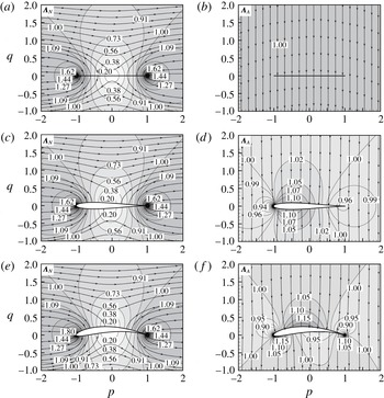
. Figure 2(a–f) displays the vortex force maps of normal and axial forces for these airfoils.
Vortex force maps displaying vortex normal and axial force lines of Joukowsky airfoils: (a) normal force for a flat plate, (b) axial force for a flat plate, (c) normal force for a symmetric Joukowsky airfoil, (d) axial force for a symmetric Joukowsky airfoil, (e) normal force for a Joukowsky airfoil with thickness and camber, (f) axial force for a Joukowsky airfoil with thickness and camber. The lines without arrows are contours of magnitude of
 $\unicode[STIX]{x1D726}_{N}$
or
 $\unicode[STIX]{x1D726}_{A}$
, and the lines with arrows are vortex force lines locally parallel to the vector
 $\unicode[STIX]{x1D726}_{N}$
or
 $\unicode[STIX]{x1D726}_{A}$
.

Figure 2(a,c,e) is for the normal force. As in Li & Wu (Reference Li and Wu2016), each arrowed vortex force line defines the most favourable direction for a TEV (giving a positive normal force) or most unfavourable direction for an LEV (giving a negative normal force). We have the surprising results that the vortex force lines for the normal force are similar for different airfoils, meaning that the typical vortex force properties obtained for a flat plate by Li & Wu (Reference Li and Wu2016) are nearly the same for general airfoils.
Figure 2(b,d,f) is for the axial force. An LEV (TEV) provides negative (positive) axial force if it moves along or at an acute angle to the vortex drag force lines. The sign of the axial forces changes if the moving direction is reversed. We note that vortex force lines for axial forces are vertical straight lines for a flat plate, and deviate only a little from vertical straight lines for other airfoils. This means that vertically moving vortices are most important to contribute (positive or negative) axial forces.
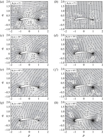
Vortex force maps displaying vortex lift (a,c,e,g) and drag (b,d,f,h) force lines of Joukowsky airfoil (with thickness
 $0.1c_{A}$
and camber
 $0.08$
) at various angles of attack. The lines without arrows are contours of magnitude of
 $\unicode[STIX]{x1D726}_{L}$
or
 $\unicode[STIX]{x1D726}_{D}$
, and the lines with arrows are vortex force lines locally parallel to the vector
 $\unicode[STIX]{x1D726}_{L}$
or
 $\unicode[STIX]{x1D726}_{D}$
.

The flat plate case may be considered as the limiting case of the Joukowsky airfoil with vanishing thickness and camber. Figure 2(a), for normal force, is the same as obtained by Li & Wu (Reference Li and Wu2016) using a different vortex force approach. Figure 2(b) is new, since Li & Wu (Reference Li and Wu2016) did not considered the axial force. It should be noted that, for a flat plate, we do not have an axial vortex (pressure) force since the plate has vanishing thickness such that there is no pressure force projection to the axial direction. For a specific flow the vortices shall organize in such a way that the overall contribution to the axial pressure force by all vortices having a vertical velocity component vanishes.
3.1.3 Vortex force maps for lift and drag
For a Joukowsky airfoil with thickness
 $0.1c_{A}$
and camber
 $0.08$
, the vortex lift/drag maps with four different angles of attack (
 $5^{\circ }$
,
 $30^{\circ }$
,
 $45^{\circ }$
,
 $60^{\circ }$
) are shown in figure 3(a–h). Panels (a,c,e,g) are for lift while panels (b,d,f,h) are for drag. For
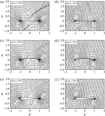
 $\unicode[STIX]{x1D6FC}=20^{\circ }$
, the vortex lift/drag maps for three different airfoils (flat plate, airfoil with zero thickness and camber
 $0.08$
, and airfoil with thickness
 $0.1c_{A}$
and zero camber) are displayed in figure 4(a–f).
Vortex force maps display vortex lift (a,c,e) and drag (b,d,f) force lines for three different airfoils: flat plate (a,b), airfoil without thickness (c,d) and airfoil without camber (e,f), for
 $\unicode[STIX]{x1D6FC}=20^{\circ }$
.

Compared to the vortex normal and axial force maps, the vortex force lines for lift and drag, which depend on the angle of attack according to (2.15), appear to have rotated in the counterclockwise direction according to the magnitude of angle of attack (at least approximately). As for the normal force, there is a region above the middle of the airfoil where the magnitude of
 $\unicode[STIX]{x1D6EC}_{L}$
is small (with a point on the airfoil having
 $\unicode[STIX]{x1D6EC}_{L}=0$
) if the angle of attack is small, and this region shifts to the leading edge when the angle of attack increases.
A similar region with small
 $\unicode[STIX]{x1D6EC}_{D}$
exists above the trailing edge at small angle of attack and this region shifts to the middle for increasing angle of attack.
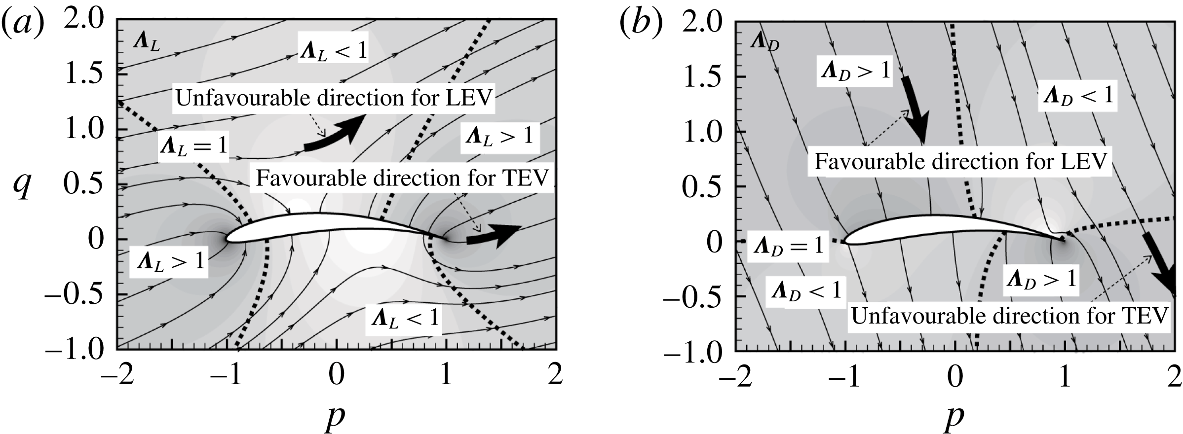
Schematic display of favourable and unfavourable directions of vortex moving in producing lift (a) and drag (b).

A schematic display of vortex lift and drag force maps is provided in figure 5. Each arrowed vortex force line in figure 5(a) defines the most favourable direction for a TEV to increase the lift or the most unfavourable direction for an LEV to decrease the lift. If moving in the opposite direction, each arrowed vortex force line defines the most unfavourable direction for a TEV to decrease the lift or the most favourable direction for an LEV to increase the lift. The lift is proportional to the magnitude of the vortex force factor (the contour lines for this magnitude are displayed as non-arrowed lines, a dashed line is used for
 $\unicode[STIX]{x1D6EC}_{L}=1$
) and the speed of the vortex. If a vortex moves at some acute or obtuse angle to the vortex force line, it is the projection of the velocity along the vortex force line that accounts for the magnitude of the lift force. Using such a map, the lift-increasing or lift-decreasing effect of a given vortex can be identified according to its circulation (sign and magnitude), position and direction.
In figure 5(b), favourable direction means negative drag (thrust) and unfavourable direction means positive drag. An LEV provides negative drag (thrust) if it moves along the favourable direction and positive drag if it moves along the opposite direction.
In conclusion, the vortex lift map is similar to the vortex force map (normal force) of a flat plate. Hence, similarly as for a flat plate, there are critical regions near the leading and trailing edges for lift enhancement. Drag force lines intersect lift force lines at a large angle, meaning that the favourable direction is different for lift and drag. A vortex does not necessarily produce lift and drag, it may produce negative lift or propulsion, depending on the direction of movement, position and the sign of circulation. Vortex force lines are dense in regions near the leading and trailing edges, meaning that vortices crossing leading edge and trailing edge regions lead to fast variation of the corresponding forces.
3.2 Vortex force study of the NACA0012 airfoil
In contrast to the Joukowsky airfoil, for which there is analytical solution to
 $\unicode[STIX]{x1D719}_{N}$
and
 $\unicode[STIX]{x1D719}_{A}$
, we have to obtain
 $\unicode[STIX]{x1D719}_{N}$
and
 $\unicode[STIX]{x1D719}_{A}$
numerically for the NACA0012 airfoil. Apart from showing the vortex force map, we will use computational fluid dynamics to check the vortex force approach.
3.2.1 Vortex force map for the NACA0012 airfoil
For the NACA0012 airfoil, the Laplace equations (2.11) and (2.12) are solved numerically to give
 $\unicode[STIX]{x1D719}_{N}$
and
 $\unicode[STIX]{x1D719}_{A}$
at discrete points of a grid with 347 417 points. The commercial code CFX has a heat transfer model, which can be used as a solver of the present Laplace equation. This grid will also be used to obtain the flow and vorticity distribution by computational fluid dynamics. This numerical method is validated by comparing the numerical solution and analytical solution using the Joukowsky airfoil. For instance, for the Joukowsky airfoil with thickness
 $0.1c_{A}$
and camber
 $0.08$
at several angles of attack, the vortex force maps with
 $\unicode[STIX]{x1D719}_{N}$
and
 $\unicode[STIX]{x1D719}_{A}$
obtained by the CFX Laplace solver are the same as the analytical vortex force maps shown by figure 3. The vortex force factors are then computed by (2.15).
Figure 6 displays the vortex force maps for both lift and drag of the NACA0012 airfoil at angles of attack
 $20^{\circ }$
and
 $60^{\circ }$
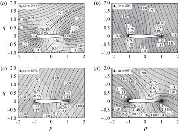
. The results are very similar to that of a Joukowsky airfoil without camber, as displayed in figures 3(e,f) and 4(e,f). This further shows that the vortex force maps are not sensitive to the shape of the airfoil.
Vortex force maps displaying vortex lift and drag force lines for NACA0012: (a) lift (
 $\unicode[STIX]{x1D6FC}=20^{\circ }$
), (b) drag (
 $\unicode[STIX]{x1D6FC}=20^{\circ }$
), (c) lift (
 $\unicode[STIX]{x1D6FC}=60^{\circ }$
), (d) drag (
 $\unicode[STIX]{x1D6FC}=60^{\circ }$
).

3.2.2 Vortex lift and drag for viscous flow around the NACA0012 airfoil
As discussed in § 2.3, the vortex force approach may be also applied to obtain vortex forces for problems where the velocity and vorticity can be given by some methods such as discrete vortex simulation and experimental measurement. The current purpose of this paper is just to study the accuracy of the approach. Note that Howe’s original approach needs further exploration since only few works have been devoted to using it in applications of airfoil aerodynamics (Hsieh et al. Reference Hsieh, Kung, Chang and Chu2010; Lee et al. Reference Lee, Hsieh, Chang and Chu2012; Li & Lu Reference Li and Lu2012). The primary purpose here is to use CFD to test the decomposed force approach given in § 2.2, which is suitable since it was devised to work in truncated domain.
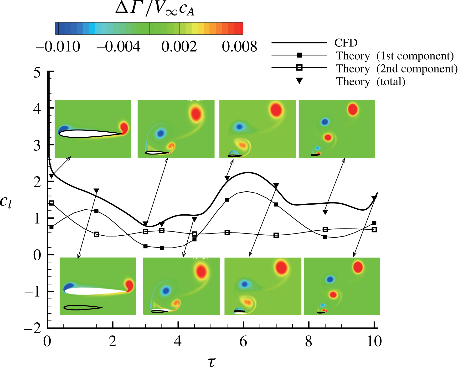
Comparison between theory and CFD for time-dependent lift coefficients and the circulation distributions at typical instants for NACA0012 flow at
 $\unicode[STIX]{x1D6FC}=60^{\circ }$
and
 $Re=1000$
. The first and second components correspond to
 $L^{(1)}$
and
 $L^{(2)}$
in expression (2.22) while the total lift coefficient is the sum of the two. Fitted curves for the first and second theoretical components, based on splines of Tecplot, have no physical meaning here and are used just to make the two components and the total one distinguishable in the picture.

The NACA0012 airfoil is used here as a test case, with
 $\overline{\boldsymbol{U}}$
and vorticity
 $\unicode[STIX]{x1D714}_{z}$
obtained by CFD. The decomposed vortex force approach, with vortex lift and drag given by (2.22) and (2.23), and the vortex force factors by (2.24) and (2.25), is applied to obtain the lift and drag. These lift and drag values will be compared to the lift and drag obtained by the CFD code – the latter are obtained from integration of the body surface pressure.
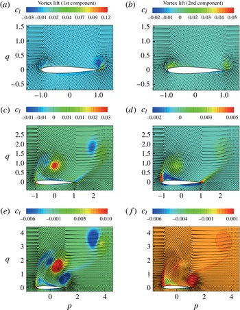
Contours of vortex lift distribution displaying forces contributed by local vortices, for a NACA0012 airfoil starting flow at instants
 $\unicode[STIX]{x1D70F}=0.125$
,
 $\unicode[STIX]{x1D70F}=1.5$
and
 $\unicode[STIX]{x1D70F}=3$
. (a,c,e) Contours of lift distribution caused by the first component. (b,d,f) Contours of lift distribution caused by the second component. The arrowed lines denote velocity vectors.

Here we only consider viscous flow so that the Kutta–Joukowsky components
 $L^{(B)}$
and
 $D^{(B)}$
vanish. The total lift coefficient and drag coefficient, defined as
 $$\begin{eqnarray}c_{l}={\displaystyle \frac{L}{{\textstyle \frac{1}{2}}\unicode[STIX]{x1D70C}V_{\infty }^{2}c_{A}}},\quad c_{d}={\displaystyle \frac{D}{{\textstyle \frac{1}{2}}\unicode[STIX]{x1D70C}V_{\infty }^{2}c_{A}}},\end{eqnarray}$$
will be displayed. Both contain two components (called first and second components here) according to (2.22) and (2.23). The forces are time-dependent and will be displayed as functions of the non-dimensional time
 $\unicode[STIX]{x1D70F}=tV_{\infty }/c_{A}$
, which measures the number of chords travelled.
For CFD, the Navier–Stokes equations in unsteady laminar flow are solved numerically using the same method as used by Li & Wu (Reference Li and Wu2016). It consists of using the commercial code Fluent with the options of a second-order upwind SIMPLE (semi-implicit method for pressure-linked equations) pressure–velocity coupling method. The computational domain is 31 chord lengths in the horizontal direction and 20 chord lengths in the vertical direction. A mesh with 104 grids on the surface of the airfoil and with 347 417 grid points in total is used. The grid size normal to the wall and in the region close to the wall is very fine. The flow is impulsively started from an initially uniform flow. The flow is unsteady and the present vortex force method should be capable of describing the vortex force at any instant, even when some early shed vortices have moved very far away from the body.
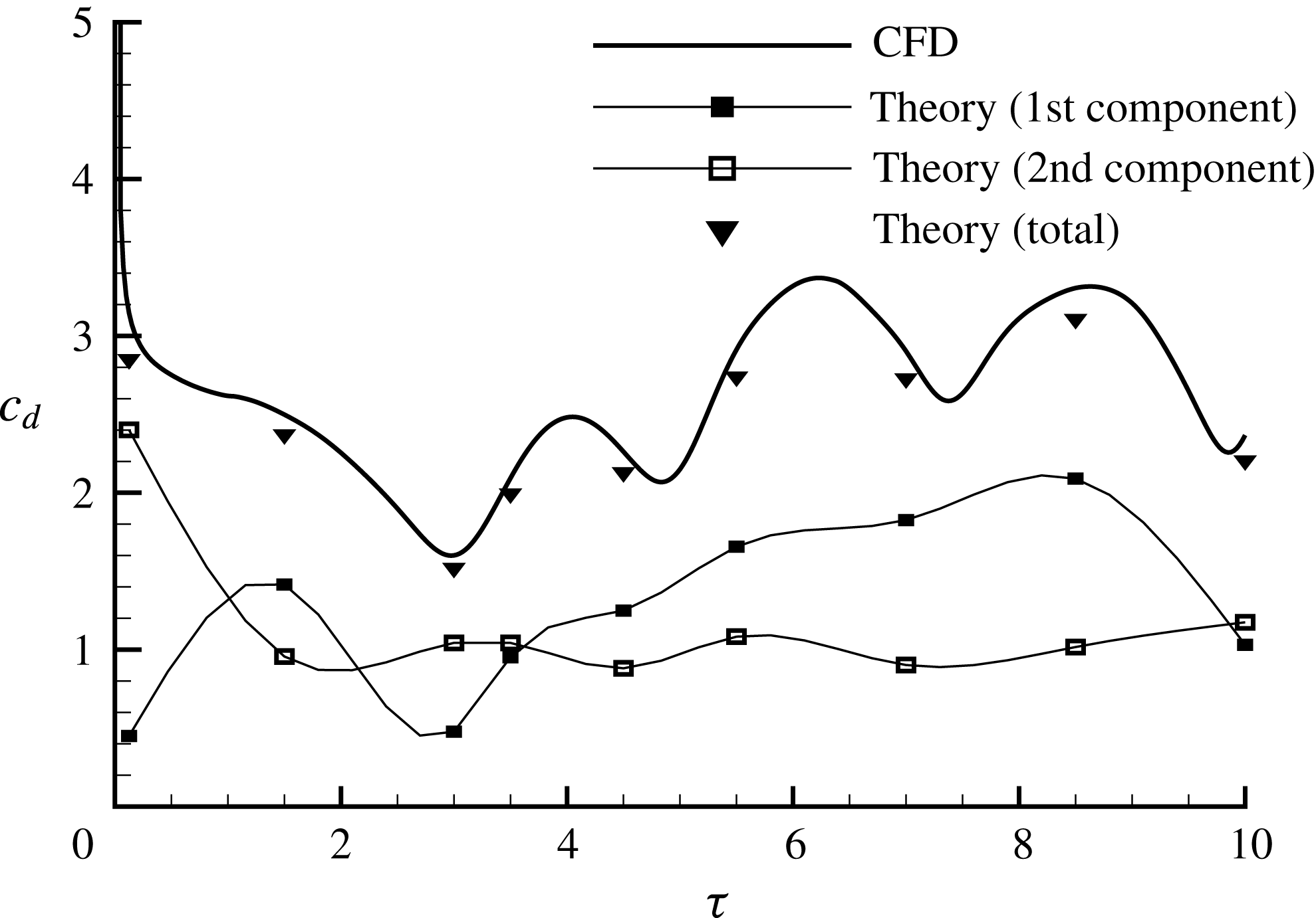
Comparison between theory and CFD for time-dependent drag coefficients for NACA0012 flow at
 $\unicode[STIX]{x1D6FC}=60^{\circ }$
and
 $Re=1000$
. The first and second components correspond to
 $D^{(1)}$
and
 $D^{(2)}$
in expression (2.23) while the total lift coefficient is the sum of the two.

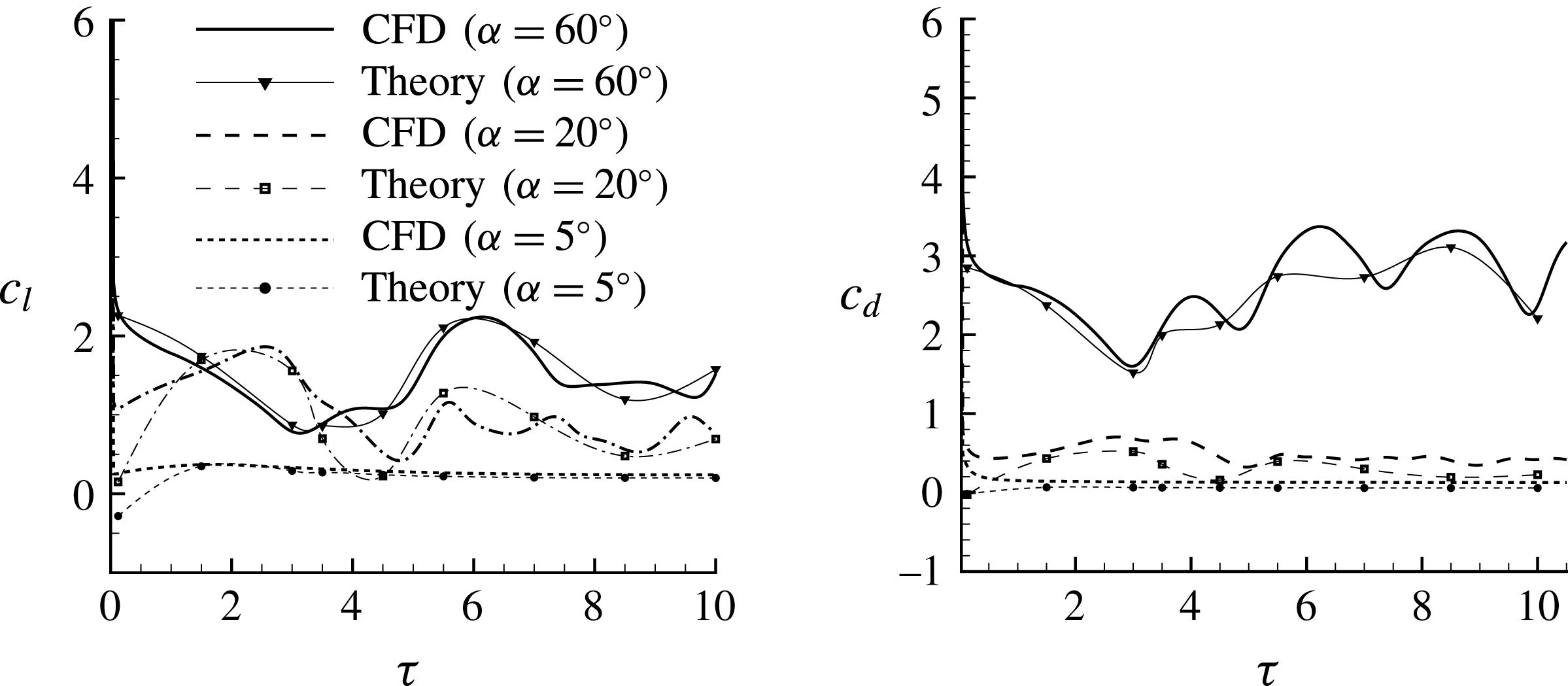
Comparison between theory and CFD for time-dependent lift and drag coefficients for NACA0012 airfoil flow at
 $Re=1000$
and at different angles of attack.

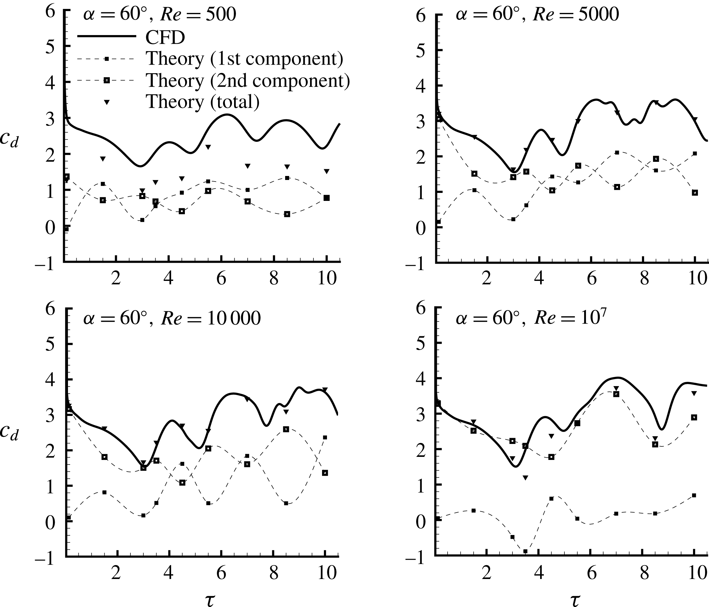
Comparison between theory and CFD for time-dependent drag coefficients for NACA0012 airfoil flow at
 $\unicode[STIX]{x1D6FC}=60^{\circ }$
and at different Reynolds numbers.

First, we choose an angle of attack
 $\unicode[STIX]{x1D6FC}=60^{\circ }$
and a Reynolds number
 $Re=1000$
.
The total lift coefficient and its two components at a series of instants are displayed in figure 7, where we also displayed the vorticity field (in terms of the non-dimensional circulation
 $(\unicode[STIX]{x0394}\unicode[STIX]{x1D6E4}/V_{\infty }c_{A})$
obtained by CFD, here
 $\unicode[STIX]{x0394}\unicode[STIX]{x1D6E4}$
is the circulation of vortices in each grid cell, defined by
 $\unicode[STIX]{x1D714}_{z}$
multiplied by the grid cell area). It is seen that the total lift coefficient
 $c_{l}$
computed by the vortex force approach compares well with the CFD lift (by integration of surface pressure).
The theoretical lift coefficient has been obtained by summing the lift coefficients of vortices inside all grid cells.
The space distribution of local lift force due to vortices inside each grid cell is displayed in figure 8. A similar approach, without force decomposition, has been used by Lee et al. (Reference Lee, Hsieh, Chang and Chu2012) to study the vortex contribution of various regions. For the first component, which depends on the local velocity, the contribution by each concentrated vortex is divided into a positive part (red colour) and a negative part (blue colour). Such a division is artificial due to the approach used, and the role of each concentrated vortex should be considered by summing the effects of these two parts. With the decomposed force approach, those vortices that are close to the airfoil contribute to the most lift. The present method thus reflects the fact that near-body vortices are more likely to induce pressure (thus lift) variation according to the Biot–Savart law. The second is that the major contribution for the second lift component comes from the tips (leading edge and trailing edge) of the airfoil. The force oscillation may be associated with the vortex flow patterns and vortex force lines in the same way as in the work of Li & Wu (Reference Li and Wu2016), and the details of a similar analysis are omitted here.
The total drag coefficient and its two components at a series of instants are displayed in figure 9. It is seen that the total drag coefficient
 $c_{d}$
computed by the vortex force approach also compares well with the CFD drag (by integration of surface pressure). The drag oscillates with a larger amplitude than lift.
In figure 10 we display the comparison between theory and CFD for three angles of attack (
 $\unicode[STIX]{x1D6FC}=60^{\circ },20^{\circ }$
and
 $5^{\circ }$
) and for
 $Re=1000$
. The comparison is still acceptable.
Good comparison is also found for different Reynolds numbers, with
 $\unicode[STIX]{x1D6FC}=60^{\circ }$
, as shown in figure 11 for drag at
 $Re=500,5000,10\,000$
and
 $10^{7}$
. The comparison for small Reynolds number is not good enough because the CFD code we use only outputs the total drag (including the pressure drag and friction drag). For small Reynolds number the friction drag is also an important component which is not considered by the vortex force formula.
4 Summary
The integral force approach of Howe (Reference Howe1995) is used here to extend the vortex force approach of Li & Wu (Reference Li and Wu2016) to general airfoils and viscous flows for both lift and drag. The vortex force approach thus obtained expresses the vortex force as the vector product of the vortex force factor and the vortex velocity. The vortex force factor can be easily obtained by solving a Laplace equation (heat equation model).
Analysis based on the Joukowsky airfoil shows that the vortex force lines for the normal force are similar to that for a flat plate, meaning that the vortex force map is insensitive to the airfoil geometry, and critical regions for force production and destruction exist for general airfoils in a similar way as for a flat plate (see Li & Wu Reference Li and Wu2016 for details for such critical regions). The vortex force lines for the axial force are almost vertical.
Vortex force lines for lift and drag have directions that can be roughly obtained from rotation (by amount of angle of attack) of those for the normal and axial forces. We have designed a schematic display of the vortex force map (figure 5), by which the most favourable/unfavourable direction of an LEV/TEV to contribute lift and drag forces is made clear.
To have a force approach that is insensitive to far-away vortices, a decomposed vortex force approach is derived. This decomposed method reflects the fact that pressure loads on the airfoil are mainly due to near-body vortices according to the Biot–Savart law. This decomposed approach performs well compared to the CFD result when viscous flow around the NACA0012 airfoil is used as example.
In summary, this work generalizes the vortex force map method, originally proposed by Li & Wu (Reference Li and Wu2015, Reference Li and Wu2016) for a flat plate and inviscid flow, to general airfoils and viscous flows, and shows that vortex force lines are not sensitive to airfoil shape, so that force behaviours (oscillation, critical region) for general airfoils are similar to a flat plate. The present method can be easily extended to three-dimensional problems – see appendix A for a brief discussion.
Acknowledgements
The authors are grateful to the referees for their helpful comments which led to improvement of this manuscript. This work was supported by the Natural National Science Foundation of China (no. 11472157) and partly by the National Basic Research Program of China (no. 2012CB720205).
Appendix A. Outline of the vortex force approach for three-dimensional flow
Using the force expression (2.8) by Howe (Reference Howe1995), the vortex force
 $F_{k}$
of a rigid body in the
 $k\text{th}$
-direction due to free vortices in the body-fixed frames can be written as
 $$\begin{eqnarray}\displaystyle F_{k} & = & \displaystyle \unicode[STIX]{x1D70C}\iiint _{\unicode[STIX]{x1D6FA}}\unicode[STIX]{x1D726}_{\boldsymbol{k},\boldsymbol{z}}\boldsymbol{\cdot }(u,v)\unicode[STIX]{x1D714}_{z}\,\text{d}\unicode[STIX]{x1D6FA}+\unicode[STIX]{x1D70C}\iiint _{\unicode[STIX]{x1D6FA}}\unicode[STIX]{x1D726}_{\boldsymbol{k},\boldsymbol{x}}\boldsymbol{\cdot }(v,w)\unicode[STIX]{x1D714}_{x}\,\text{d}\unicode[STIX]{x1D6FA}\nonumber\\ \displaystyle & & \displaystyle +\,\unicode[STIX]{x1D70C}\iiint _{\unicode[STIX]{x1D6FA}}\unicode[STIX]{x1D726}_{\boldsymbol{k},\boldsymbol{y}}\boldsymbol{\cdot }(u,w)\unicode[STIX]{x1D714}_{y}\,\text{d}\unicode[STIX]{x1D6FA}.\end{eqnarray}$$
In the above expression,
 $k$
means any direction (such as normal, axial and sideward direction),
 $(u,v,w)$
are the three components of flow velocity,
 $(\unicode[STIX]{x1D714}_{x},\unicode[STIX]{x1D714}_{y},\unicode[STIX]{x1D714}_{z})$
are the three components of flow vorticity and the vortex force factors in the
 $z,x$
and
 $y$
planes are defined by
 $$\begin{eqnarray}\unicode[STIX]{x1D726}_{\boldsymbol{k},\boldsymbol{z}}=\left(-{\displaystyle \frac{\unicode[STIX]{x2202}\unicode[STIX]{x1D719}_{k}}{\unicode[STIX]{x2202}y}},{\displaystyle \frac{\unicode[STIX]{x2202}\unicode[STIX]{x1D719}_{k}}{\unicode[STIX]{x2202}x}}\right),\quad \unicode[STIX]{x1D726}_{\boldsymbol{k},\boldsymbol{x}}=\left(-{\displaystyle \frac{\unicode[STIX]{x2202}\unicode[STIX]{x1D719}_{k}}{\unicode[STIX]{x2202}z}},\quad {\displaystyle \frac{\unicode[STIX]{x2202}\unicode[STIX]{x1D719}_{k}}{\unicode[STIX]{x2202}y}}\right),\quad \unicode[STIX]{x1D726}_{\boldsymbol{k},\boldsymbol{y}}=\left({\displaystyle \frac{\unicode[STIX]{x2202}\unicode[STIX]{x1D719}_{k}}{\unicode[STIX]{x2202}z}},-{\displaystyle \frac{\unicode[STIX]{x2202}\unicode[STIX]{x1D719}_{k}}{\unicode[STIX]{x2202}x}}\right).\end{eqnarray}$$
Here,
 $\unicode[STIX]{x1D719}_{k}$
is the potential of the hypothetical flow induced by unitary motion in the
 $k\text{th}$
-direction of the ideal fluid. Let
 $\unicode[STIX]{x1D719}_{N}$
,
 $\unicode[STIX]{x1D719}_{A}$
and
 $\unicode[STIX]{x1D719}_{S}$
be the hypothetical potentials due to unitary motion along the normal (
 $z$
), axial (
 $x$
) or sideward (
 $y$
) direction, then
 $$\begin{eqnarray}\left.\begin{array}{@{}c@{}}{\displaystyle \frac{\unicode[STIX]{x2202}^{2}\unicode[STIX]{x1D719}_{N}}{\unicode[STIX]{x2202}x^{2}}}+{\displaystyle \frac{\unicode[STIX]{x2202}^{2}\unicode[STIX]{x1D719}_{N}}{\unicode[STIX]{x2202}y^{2}}}+{\displaystyle \frac{\unicode[STIX]{x2202}^{2}\unicode[STIX]{x1D719}_{N}}{\unicode[STIX]{x2202}z^{2}}}=0,\\ {\displaystyle \frac{\unicode[STIX]{x2202}\unicode[STIX]{x1D719}_{N}}{\unicode[STIX]{x2202}n}}=0\quad (x,y,z)\rightarrow S_{B},\\ {\displaystyle \frac{\unicode[STIX]{x2202}\unicode[STIX]{x1D719}_{N}}{\unicode[STIX]{x2202}x}}=0,\quad {\displaystyle \frac{\unicode[STIX]{x2202}\unicode[STIX]{x1D719}_{N}}{\unicode[STIX]{x2202}y}}=0,\quad {\displaystyle \frac{\unicode[STIX]{x2202}\unicode[STIX]{x1D719}_{N}}{\unicode[STIX]{x2202}z}}=-1\quad (x,y,z)\rightarrow \infty \end{array}\right\}\end{eqnarray}$$
 $$\begin{eqnarray}\left.\begin{array}{@{}c@{}}{\displaystyle \frac{\unicode[STIX]{x2202}^{2}\unicode[STIX]{x1D719}_{A}}{\unicode[STIX]{x2202}x^{2}}}+{\displaystyle \frac{\unicode[STIX]{x2202}^{2}\unicode[STIX]{x1D719}_{A}}{\unicode[STIX]{x2202}y^{2}}}+{\displaystyle \frac{\unicode[STIX]{x2202}^{2}\unicode[STIX]{x1D719}_{A}}{\unicode[STIX]{x2202}z^{2}}}=0,\\ {\displaystyle \frac{\unicode[STIX]{x2202}\unicode[STIX]{x1D719}_{A}}{\unicode[STIX]{x2202}n}}=0\quad (x,y,z)\rightarrow S_{B},\\ {\displaystyle \frac{\unicode[STIX]{x2202}\unicode[STIX]{x1D719}_{A}}{\unicode[STIX]{x2202}x}}=-1,\quad {\displaystyle \frac{\unicode[STIX]{x2202}\unicode[STIX]{x1D719}_{A}}{\unicode[STIX]{x2202}y}}=0,\quad {\displaystyle \frac{\unicode[STIX]{x2202}\unicode[STIX]{x1D719}_{A}}{\unicode[STIX]{x2202}z}}=0\quad (x,y,z)\rightarrow \infty \end{array}\right\}\end{eqnarray}$$
 $$\begin{eqnarray}\left.\begin{array}{@{}c@{}}{\displaystyle \frac{\unicode[STIX]{x2202}^{2}\unicode[STIX]{x1D719}_{S}}{\unicode[STIX]{x2202}x^{2}}}+{\displaystyle \frac{\unicode[STIX]{x2202}^{2}\unicode[STIX]{x1D719}_{S}}{\unicode[STIX]{x2202}y^{2}}}+{\displaystyle \frac{\unicode[STIX]{x2202}^{2}\unicode[STIX]{x1D719}_{S}}{\unicode[STIX]{x2202}z^{2}}}=0,\\ {\displaystyle \frac{\unicode[STIX]{x2202}\unicode[STIX]{x1D719}_{S}}{\unicode[STIX]{x2202}n}}=0\quad (x,y,z)\rightarrow S_{B},\\ {\displaystyle \frac{\unicode[STIX]{x2202}\unicode[STIX]{x1D719}_{S}}{\unicode[STIX]{x2202}x}}=0,\quad {\displaystyle \frac{\unicode[STIX]{x2202}\unicode[STIX]{x1D719}_{S}}{\unicode[STIX]{x2202}y}}=-1,\quad {\displaystyle \frac{\unicode[STIX]{x2202}\unicode[STIX]{x1D719}_{S}}{\unicode[STIX]{x2202}z}}=0\quad (x,y,z)\rightarrow \infty .\end{array}\right\}\end{eqnarray}$$
For a given body of any shape,
 $\unicode[STIX]{x1D719}_{N}$
,
 $\unicode[STIX]{x1D719}_{A}$
and
 $\unicode[STIX]{x1D719}_{S}$
are obtained by solving (A 3)–(A 5) numerically and then put into (A 2) to get vortex force vectors
 $\unicode[STIX]{x1D726}_{\boldsymbol{k},\boldsymbol{z}},\unicode[STIX]{x1D726}_{\boldsymbol{k},\boldsymbol{x}}$
and
 $\unicode[STIX]{x1D726}_{\boldsymbol{k},\boldsymbol{y}}$
(with
 $k=N,A$
and
 $S$
). More details are expected to be provided in future studies for specific applications.