


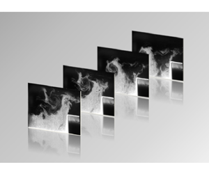
1 Introduction
Turbulent flow is ubiquitous in nature and is found across a wide range of systems that span simple flows, such as a flow in a coffee cup, to cosmological flows. The presence and significance of eddies of different length scales in turbulent flows have been studied extensively in the past few decades (Tennekes & Lumley Reference Tennekes and Lumley1972; Frisch & Kolmogorov Reference Frisch and Kolmogorov1995; Davidson Reference Davidson2015). Turbulent kinetic energy from the eddies of large length scales is transferred to lower but comparable length scales through nonlinear interactions. Eventually, the energy is dissipated as heat at the Kolmogorov length scales through viscous dissipation. This process of energy transfer across different length scales is referred to as the energy cascade (Richardson Reference Richardson1922; Pope Reference Pope2000).
The nonlinear interaction between the eddies of multiple scales causes the flow to become chaotic (Aref Reference Aref1983; McWilliams Reference McWilliams1984). However, in some turbulent flows, we can observe an emergence of order from chaos characterized by the evolution of large-scale structures formed by the roll-up or merging of several small-scale structures. These large-scale organized structures are referred to as coherent structures (Ho & Nosseir Reference Ho and Nosseir1981; McWilliams Reference McWilliams1984).
Similar to the emergence of order from chaos in turbulent flows, other systems also exhibit transition to order. Spontaneous transition from chaos to order in biological systems, ecological systems etc., has been studied extensively using the theory of self-organization (Ball Reference Ball1999; Camazine et al. Reference Camazine, Deneubourg, Franks, Sneyd, Bonabeau and Theraula2003). Cross & Hohenberg (Reference Cross and Hohenberg1993) present many examples of self-organization, both in temporal and spatial dynamics, in hydrodynamic systems such as Rayleigh–Bénard convection, Taylor–Couette flow etc.
Emergence of temporal order in systems which exhibit oscillatory instabilities often manifests as an emergence of periodicity in the temporal fluctuations of the state variable(s) of the system. Such an emergence of temporal order has been observed in aeroacoustic (Rockwell & Naudascher Reference Rockwell and Naudascher1979; Rockwell Reference Rockwell1983), aeroelastic (Fung Reference Fung1955) and thermoacoustic systems (Zukoski Reference Zukoski1985; Poinsot et al. Reference Poinsot, Trouve, Veynante, Candel and Esposito1987). In such systems, order emerges in the form of self-sustained periodic oscillations in their state variable(s).
In general, order can also emerge in the spatial domain in thermodynamically open systems, operating far from thermodynamic equilibrium. Emergence of such spatiotemporal order is often through spontaneous self-organization, achieved by the exchange of energy and matter with the external environment (Tiezzi et al. Reference Tiezzi, Pulselli, Marchettini and Tiezzi2008). Examples of systems that exhibit such self-organization include Belousov–Zhabotinsky reaction, Bénard cells and droplet clusters (Tiezzi et al. Reference Tiezzi, Pulselli, Marchettini and Tiezzi2008; Ciotti et al. Reference Ciotti, Budroni, Masia, Marchettini and Rustici2011).
Such an emergence of order from chaos is observed in a turbulent thermoacoustic system during the transition from the state of combustion noise to thermoacoustic instability. The state of combustion noise corresponds to the stable operating regime of the combustor (Strahle Reference Strahle1978), while thermoacoustic instability corresponds to the unstable operating regime of the combustor. Thermoacoustic instability occurs due to a positive feedback between the unsteady heat release rate and the acoustic pressure oscillations and is characterized by large amplitude pressure oscillations which lead to excessive structural vibrations (Lieuwen Reference Lieuwen2012; Juniper & Sujith Reference Juniper and Sujith2018).
Recent studies indicate that the transition states prior to thermoacoustic instability exhibit rich dynamic behaviour (Gotoda et al. Reference Gotoda, Nikimoto, Miyano and Tachibana2011, Reference Gotoda, Okuno, Hayashi and Tachibana2015; Nair, Thampi & Sujith Reference Nair, Thampi and Sujith2014; Unni & Sujith Reference Unni and Sujith2015; Pawar et al. Reference Pawar, Seshadri, Unni and Sujith2017). A turbulent combustor exhibits the characteristics of a complex system during these states (Juniper & Sujith Reference Juniper and Sujith2018; Unni et al. Reference Unni, Krishnan, Manikandan, George, Sujith, Marwan and Kurths2018). Results from these studies indicate that there is a gradual emergence of periodicity from aperiodicity in the temporal dynamics (Nair et al. Reference Nair, Thampi and Sujith2014) and an emergence of order from disorder in the spatiotemporal dynamics during the transition from combustion noise to thermoacoustic instability via intermittency (Mondal, Unni & Sujith Reference Mondal, Unni and Sujith2017; George et al. Reference George, Unni, Raghunathan and Sujith2018; Premchand et al. Reference Premchand, George, Raghunathan, Unni, Sujith and Nair2019). During the occurrence of intermittency, bursts of high amplitude periodic fluctuations appear amidst epochs of low amplitude aperiodic fluctuations in an apparently random manner.
The spatiotemporal dynamics of a turbulent combustor is largely influenced by the coupling between the various subsystems such as the hydrodynamic field, the reactive field (flame) and the acoustic field (Candel Reference Candel1992). George et al. (Reference George, Unni, Raghunathan and Sujith2018) showed that the emergence of order from chaos during thermoacoustic instability is the result of interactions among the patterns formed in various subsystems. The patterns formed are the standing wave pattern in the acoustic field, the large-scale coherent structures in the flow field and the coherent patterns of the flame. They suggested that interactions between these subsystems are mediated by the emerging spatiotemporal patterns, leading to increased order or coherence in the combustion dynamics. For instance, they showed that collective interaction of small-scale vortices results in the formation of a large-scale vortex and leads to coherence in the flame.
Richardson’s (Reference Richardson1922) description of turbulent flows states that flows consist of a hierarchy of scales. Several studies showed that flow structures with multiple spatial scales in turbulent flows exhibit the characteristics of self-similarity (Meneveau & Sreenivasan Reference Meneveau and Sreenivasan1986; Benzi et al. Reference Benzi, Ciliberto, Tripiccione, Baudet, Massaioli and Succi1993). The self-similarity in turbulent flows has been studied using the theory of fractal geometry. For example, Mandelbrot (Reference Mandelbrot1983) suggested that turbulence involves several fractal facets. Fractal theory gives us a simple, geometrical interpretation of the complexity in the system.
The complexity exhibited by many spatially extended systems is due to the presence of multiple spatial and temporal scales. In such systems, a spectrum of fractal dimensions is required to characterize their complexity (Murcio et al. Reference Murcio, Masucci, Arcaute and Batty2015). Such a system characterized by a set of fractal dimensions is referred to as a multifractal system. If a fractal can be described using a single fractal dimension, then it is called a monofractal. Otherwise, it is labelled as a multifractal (Engelking Reference Engelking1978; Pesin Reference Pesin2008). Examples of multifractal time series include human physiological signals (Ivanov et al. Reference Ivanov, Amaral, Goldberger, Havlin, Rosenblum, Struzik and Stanley1999; Ihlen & Vereijken Reference Ihlen and Vereijken2013), geoelectric signals (Telesca et al. Reference Telesca, Colangelo, Lapenna and Macchiato2003) and seismic signals (Telesca et al. Reference Telesca, Lovallo, Molist, Moreno and Meléndez2015). Multifractal description was first introduced by Mandelbrot to study the fractal characteristics of turbulent flows (Mandelbrot Reference Mandelbrot1974). Meneveau & Sreenivasan (Reference Meneveau and Sreenivasan1991) experimentally showed that the kinetic energy dissipation field in a turbulent flow has a multifractal distribution which supports the notion of a self-similar multiplicative fragmentation process occurring in the energy cascade.
For a swirl-stabilized turbulent combustor, Gotoda et al. (Reference Gotoda, Amano, Miyano, Ikawa, Maki and Tachibana2012) showed that the acoustic pressure oscillations prior to lean blowout exhibit multifractal characteristics. In addition, they also emphasized that multifractal analysis is indeed necessary to capture the rich dynamics observed in the pressure oscillations near to the blowout. For bluff-body stabilized and swirl-stabilized turbulent combustors, Nair & Sujith (Reference Nair and Sujith2014) reported that the unsteady pressure oscillations exhibit multifractality due to the presence of fluctuations of multiple temporal scales during the occurrence of combustion noise. Further, they showed that there is a loss of multifractality in the unsteady pressure oscillations when the combustion dynamics transitions from combustion noise to thermoacoustic instability. This loss of multifractality was attributed to a reduction of multiple time scales to a few discrete time scales associated with the formation of a large-scale coherent structure during the occurrence of thermoacoustic instability. However, the above studies did not discuss the multifractal characteristics associated with the flame dynamics.
In the present work, we study multifractality of the flame topology as the dynamical state of a turbulent thermoacoustic system transitions from combustion noise to thermoacoustic instability via intermittency. We observe small-scale vortical structures during the occurrence of combustion noise and a wide range of spatial scales during the occurrence of thermoacoustic instability. We show that the turbulent flame topology exhibits multifractality during the different dynamical states. Even during the occurrence of thermoacoustic instability when there is an existence of ordered temporal dynamics, the spatial topology of the flame is multifractal. We show that periodic oscillations of the multifractal spectrum of the flame topology result in the periodic oscillations of the heat release rate.
The paper is organized as follows: § 2 presents a background of the multifractal formalism. Section 3 provides the details of the experimental set-up and the data acquisition systems used in this study. Section 4 discusses the results from the experimental study. Section 5 presents the key findings of the study. A comparison of the turbulent spatial scales with other spatial scales in the system, methodology to detect the flame contours, the estimation of the multifractal spectrum and the uncertainties estimation in the calculation of multifractal parameters are elaborated in the appendices A–D, respectively.
2 Multiplicative cascade processes and multifractality
Many natural processes such as cloud formation, nuclear chain reaction, turbulent flows, redistribution of human population across the globe, biological evolution etc., involve multiplicative cascade processes (Schertzer et al. Reference Schertzer, Lovejoy, Schmitt, Chigirinskaya and Marsan1997; Cheng Reference Cheng2014). A multiplicative cascade process is characterized by iterative transformations of a system resulting in the redistribution of a measure of the system across its topology. Here, the measure is any quantifiable property of the system such as population density, concentration of a species, energy density etc., that varies across the topology of the system. A famous example of a multiplicative cascade process is the turbulent energy cascade (Richardson Reference Richardson1922). The multiplicative cascade process often results in a fractal or multifractal distribution of a measure across the topology of a system (Martínez et al. Reference Martínez, Jones, Domínguez-Tenreiro and Weygaert1990).
Fractals are geometric objects that are self-similar across different scales. Measures such as length and area of a fractal are dependent upon the scale of the measurement. A log–log plot of a measure of the fractal with the scale of the measurement gives a straight line with a non-integer slope of negative fractal dimension. In systems with heterogeneous distribution of measures such as the distribution of copper ore in the earth’s crust (Mandelbrot Reference Mandelbrot1989), distribution of rainfall and clouds across the atmosphere (Lovejoy & Schertzer Reference Lovejoy and Schertzer1991), the scaling behaviour can vary from one part of the system to another. For such systems, a single fractal dimension is inadequate to explain the local scaling behaviours of the measure and a multifractal description is needed to represent the complexity in the scaling. Often, in spatiotemporal systems, the local fractal dimension could vary in space due to the localized irregularities in the field, making them multifractal (Dauphiné Reference Dauphiné2013).
Classical statistical properties such as variance, skewness and kurtosis, represent the statistical dispersion of a measure. However, these properties do not account for the non-stationarity and the non-homogeneity in the distribution of a measure. In multifractal analysis, it is possible to determine the irregularities and discontinuities present in the spatial distribution of a measure. A multifractal spectrum represents all such irregularities, large or small, across all scales of the measure, based on the scaling of different orders of moments of the distribution of the measure (Salat, Murcio & Arcaute Reference Salat, Murcio and Arcaute2017). In this study we use a multifractal spectrum known as the singularity spectrum, obtained using the box-counting method, to study the multifractal characteristics of the flame topology.
In a multifractal field  $G$, a measure (
 $\unicode[STIX]{x1D707}$) which characterizes the topology of
 $G$ varies in space. A mathematical description of measure
 $\unicode[STIX]{x1D707}$ is explained in appendix C. Consider a region of radius,
 $\unicode[STIX]{x1D700}$ around any point,
 $x_{0}$ in
 $G$. The measure
 $\unicode[STIX]{x1D707}$ within the region of radius
 $\unicode[STIX]{x1D700}$ has a power-law relation with
 $\unicode[STIX]{x1D700}$, when the range of
 $\unicode[STIX]{x1D700}$ is sufficiently small (Chhabra & Jensen Reference Chhabra and Jensen1989). Accordingly, the relation between
 $\unicode[STIX]{x1D707}$ and
 $\unicode[STIX]{x1D700}$ is given as
 $$\begin{eqnarray}\unicode[STIX]{x1D707}(\unicode[STIX]{x1D700})\sim \unicode[STIX]{x1D700}^{\unicode[STIX]{x1D6FC}},\end{eqnarray}$$
where the scaling exponent  $\unicode[STIX]{x1D6FC}$ is known as the Lipschitz–Hölder exponent. The exponent
 $\unicode[STIX]{x1D6FC}$ represents the strength of the local scaling of the distribution of
 $\unicode[STIX]{x1D707}$ around
 $x_{0}$, otherwise known as the singularity exponent at
 $x_{0}$. Since
 $G$ is multifractal,
 $\unicode[STIX]{x1D6FC}$ is a function of
 $x_{0}$. The distribution of
 $\unicode[STIX]{x1D6FC}$ in
 $G$ is characterized by
 $f(\unicode[STIX]{x1D6FC})$, which is the fractal dimension (Hausdorff dimension) corresponding to the set of points in
 $G$ with a singularity exponent
 $\unicode[STIX]{x1D6FC}$. The fractal dimension
 $f(\unicode[STIX]{x1D6FC})$ for a given
 $\unicode[STIX]{x1D6FC}$ is determined based on the number of regions
 $N_{\unicode[STIX]{x1D6FC}}(\unicode[STIX]{x1D700})$ of radius
 $\unicode[STIX]{x1D700}$ that form the set with the same
 $\unicode[STIX]{x1D6FC}$ and is given as,
 $$\begin{eqnarray}N_{\unicode[STIX]{x1D6FC}}(\unicode[STIX]{x1D700})\sim \unicode[STIX]{x1D700}^{-f(\unicode[STIX]{x1D6FC})}.\end{eqnarray}$$
In the present work, we compute  $\unicode[STIX]{x1D6FC}$ and
 $f(\unicode[STIX]{x1D6FC})$ following the method described by Chhabra & Jensen (Reference Chhabra and Jensen1989). The steps for the estimation of
 $\unicode[STIX]{x1D6FC}$ and
 $f(\unicode[STIX]{x1D6FC})$ are explained in appendix C. In our analysis,
 $\unicode[STIX]{x1D707}$ is selected as the normalized probability mass distribution of the non-zero pixel intensity in the flame image (Giri et al. Reference Giri, Tarafdar, Gouze and Dutta2014).
The singularity spectrum  $f(\unicode[STIX]{x1D6FC})$ is plotted as a function of the singularity exponent
 $\unicode[STIX]{x1D6FC}$. The singularity spectrum is obtained by performing multifractal analysis on a typical flame image obtained in our experiments. The parameters
 $D_{0}$,
 $\unicode[STIX]{x1D6FC}_{0}$,
 $\unicode[STIX]{x0394}\unicode[STIX]{x1D6FC}_{right}$,
 $\unicode[STIX]{x0394}\unicode[STIX]{x1D6FC}_{left}$ and
 $W$ define the multifractal spectrum.

The multifractal spectrum provides a mathematical description of multifractality in terms of  $f(\unicode[STIX]{x1D6FC})$ and
 $\unicode[STIX]{x1D6FC}$. Figure 1 shows the representative multifractal spectrum resulting from the multifractal analysis on a flame image acquired in our experiments. The shape and the position of the spectrum represents the range of fractal dimensions required to describe the system and the relative dominance of each fractal dimension in determining its topology. For the case of monofractals, the multifractal spectrum reduces to a point as
 $\unicode[STIX]{x1D6FC}$ becomes constant everywhere.
The four parameters namely, the capacity dimension  $D_{0}$, the spectrum width
 $W$, the most dominant singularity exponent
 $\unicode[STIX]{x1D6FC}_{0}$ (value of
 $\unicode[STIX]{x1D6FC}$ at which
 $f(\unicode[STIX]{x1D6FC})$ is maximum) and the asymmetry parameter
 $B$ are used to characterize the multifractal spectrum (Telesca et al. Reference Telesca, Colangelo, Lapenna and Macchiato2003). The maximum value of
 $f(\unicode[STIX]{x1D6FC})$ is the capacity dimension (
 $D_{0}$) which quantifies the space-filling nature of the fractal. For example, a fractal curve that lies in a two-dimensional (2-D) plane is said to be space-filling if the curve is highly wrinkled and hence covers most of the area of the 2-D plane. The
 $D_{0}$ of such a 2-D fractal object lies in the interval between 1 and 2. A high value of
 $D_{0}$ close to 2 indicates that the space is almost entirely occupied by the fractal (Lopes & Betrouni Reference Lopes and Betrouni2009). Conversely,
 $D_{0}$ reduces to 1 for a line segment. We further state that the capacity dimension or the box-counting dimension (calculated using the box-counting method) takes the same value as the Hausdorff dimension, when the fractal satisfies the open set condition (Wagon Reference Wagon2010).
The width of the spectrum defined as  $W=\unicode[STIX]{x1D6FC}_{max}-\unicode[STIX]{x1D6FC}_{min}$, represents the range of scaling exponents found in the multifractal field
 $G$. The larger the value of
 $W$, the wider the range of scaling exponents present in
 $G$. The most dominant singularity exponent
 $\unicode[STIX]{x1D6FC}_{0}$ represents the most probable singularity over the support of
 $G$ (Goltz Reference Goltz1996; Giri et al. Reference Giri, Tarafdar, Gouze and Dutta2014). A high value of
 $\unicode[STIX]{x1D6FC}_{0}$ indicates a higher probability of regions of densely concentrated
 $\unicode[STIX]{x1D707}$ over the support of
 $G$. Conversely, a low value of
 $\unicode[STIX]{x1D6FC}_{0}$ indicates a high probability of regions of sparse distribution of
 $\unicode[STIX]{x1D707}$ over the support of
 $G$.
The asymmetry parameter  $B$ describes the skewness of the spectrum based on
 $\unicode[STIX]{x0394}\unicode[STIX]{x1D6FC}_{right}$ and
 $\unicode[STIX]{x0394}\unicode[STIX]{x1D6FC}_{left}$, where
 $\unicode[STIX]{x0394}\unicode[STIX]{x1D6FC}_{right}$ is given as
 $\unicode[STIX]{x1D6FC}_{max}-\unicode[STIX]{x1D6FC}_{0}$ and
 $\unicode[STIX]{x0394}\unicode[STIX]{x1D6FC}_{left}=\unicode[STIX]{x1D6FC}_{0}-\unicode[STIX]{x1D6FC}_{min}$. The asymmetry parameter is defined as
 $B=\unicode[STIX]{x0394}\unicode[STIX]{x1D6FC}_{right}-\unicode[STIX]{x0394}\unicode[STIX]{x1D6FC}_{left}$. The spectrum is symmetric if
 $B=0$, left-skewed if
 $B$ is negative and right-skewed if
 $B$ is positive. A right-skewed spectrum indicates more irregularity within the smaller spatial structures. Conversely, a left-skewed spectrum indicates higher irregularity within the larger spatial structures.
In the present work, we estimate the values of  $D_{0}$,
 $\unicode[STIX]{x1D6FC}_{0}$,
 $W$ and
 $B$ of the flame contours. These flame contours are extracted from the Mie scattering images of the reactive flow. The flame contains wrinkles which are heterogeneously distributed. We study the spatial distribution of these wrinkles in the flame during the different dynamical states. The above-mentioned multifractal parameters can be used to describe the multifractal characteristics of the flame. The capacity dimension
 $D_{0}$ represents the space-filling nature of the flame inside the combustor. A high value of
 $D_{0}$ indicates that wrinkles in the flame occupy a larger area in the combustor. The most dominant singularity exponent
 $\unicode[STIX]{x1D6FC}_{0}$ represents how the distribution of wrinkles is present over the flame. A high value of
 $\unicode[STIX]{x1D6FC}_{0}$ indicates a heterogeneous concentration of wrinkles, with certain regions having dense concentration compared to other regions. The width of the spectrum demonstrates the range of scaling required to describe the distribution of wrinkles in the flame. A larger value of
 $W$ implies that a wider range of scaling exponents is required to describe the distribution of wrinkles. The skewness indicates the dominance of irregularities either for the smaller length scales or for the larger length scales.
3 Experimental set-up
Experiments were performed on a turbulent combustor where the flame is stabilized using a circular bluff-body, at high Reynolds numbers ( $Re>18\,000$). The turbulent combustor used for the present study is shown in figure 2. The turbulent combustor consists of a plenum chamber, a burner and a combustion chamber with extension ducts. A central shaft of diameter 16 mm through the burner supports the bluff-body. The central shaft is also used to deliver fuel into the combustion chamber through four radial injection holes of diameter 1.7 mm. The fuel is injected 120 mm upstream of the bluff-body. The bluff-body is a circular disk of diameter 47 mm and thickness 10 mm. The bluff-body is located at a fixed position of 35 mm from the backward facing step of the combustor. A disk of 2 mm thickness with 300 holes of diameter 1.7 mm each, located 30 mm downstream of the location of fuel-injection acts as a flashback arrestor. The combustion chamber consists of a sudden expansion from the circular burner of diameter 40 mm into a square geometry of cross-section 90 mm
 $\times$ 90 mm and length 1100 mm. A spark plug with a step-up transformer is mounted near the dump plane for ignition of the fuel–air mixture. We use liquefied petroleum gas (60 % butane and 40 % propane) as the fuel. A blow-down mechanism is used to supply air from high-pressure tanks. The air is passed through a moisture separator before it enters the plenum chamber.
Schematic of the turbulent combustor used in this study. A piezoelectric pressure transducer measures the acoustic pressure fluctuations ( $p^{\prime }$) whereas a photomultiplier (PMT) records the global heat release rate (
 $\dot{q}$). Mie scattering images of seeding particles (
 $\text{TiO}_{2}$), in a reactive flow are captured using a high-speed camera.

The mass flow rates of air and fuel are controlled and measured using mass flow controllers (Alicat Scientific, MCR Series) with an uncertainty of  $\pm$ (0.8 % of reading
 $+0.2\,\%$) of full scale. The Reynolds number for the reactive flow is computed using the expression
 $Re=4{\dot{m}}/\unicode[STIX]{x03C0}\unicode[STIX]{x1D707}_{a}(d_{o}-d_{i})$, where
 ${\dot{m}}={\dot{m}}_{a}+{\dot{m}}_{f}$ is the mass flow rate of the air–fuel mixture,
 $d_{o}$ is the diameter of the burner,
 $d_{i}$ is the diameter of the bluff-body shaft and
 $\unicode[STIX]{x1D707}_{a}$ is the dynamic viscosity of the air–fuel mixture at the experimental conditions (Holman Reference Holman1989). Further, the total mass flow rate of air for the combustion is given as
 ${\dot{m}}_{a}={\dot{m}}_{s}+{\dot{m}}_{m}$, where
 ${\dot{m}}_{s}$ and
 ${\dot{m}}_{m}$ are the mass flow rates of the seeded and unseeded air streams, respectively. Corrections to Reynolds number due to the change in viscosity for the varying air–fuel ratios are performed, the procedure for which can be found in Wilke (Reference Wilke1950). The Reynolds numbers for the reported experiments are
 $Re=1.88\times 10^{4}\pm 574$ (combustion noise),
 $2.2\times 10^{4}\pm 630$ (intermittency) and
 $3.15\times 10^{4}\pm 889$ (thermoacoustic instability). The required Reynolds number is achieved by maintaining a constant fuel flow rate (30 standard litres per minute) and increasing the air flow rate. In this study, we discuss the results obtained at different equivalence ratios (
 $\unicode[STIX]{x1D719}$). The global equivalence ratio is calculated as
 $({\dot{m}}_{f}/{\dot{m}}_{a})_{actual}/({\dot{m}}_{f}/{\dot{m}}_{a})_{stoichiometry}$. The uncertainty present in the equivalence ratio is
 $\pm 0.02$ based on the uncertainties in the mass flow controllers.
To maintain a certain level of consistency in the environmental conditions, experiments were performed when the acoustic damping rate is  $19~\text{s}^{-1}\pm 15\,\%$. The unsteady pressure signals are acquired using piezoelectric pressure transducers (PCB103B02, uncertainty
 $\pm 0.15~\text{Pa}$). This pressure transducer is mounted at a distance of 25 mm from the dump plane of the combustor as shown in figure 2. A photomultiplier (PMT) (Hamamatsu H10722-01) with an OH* filter (narrow bandwidth filter centred at 310 nm and 12 nm full width at half maximum) mounted in front of it, is used to capture the chemiluminescence intensity which is indicative of the global heat release rate within the combustor (Hardalupas & Orain Reference Hardalupas and Orain2004). The PMT is positioned such that the intensity of chemiluminescence from the entire flame in the combustion chamber is captured. Both the pressure signal from the pressure transducer and the global heat release rate from the PMT are acquired using an analogue-to-digital card (NI-6143, 16 bit) for a duration of 3 s with a sampling rate of 20 kHz. The acquisition of the pressure signals, PMT signals and camera images is synchronized using a signal generator (Tektronix-AFG1022, 25 MHz).
We acquired simultaneous 2-D planar Mie scattering images, acoustic pressure and global heat release rate measurements at different values of  $\unicode[STIX]{x1D719}$ from stoichiometric conditions to leaner conditions. Thermoacoustic instability is observed at leaner conditions. For the 2-D planar Mie scattering technique, we use a single-cavity double-pulsed Nd:YLF laser (Photonics) of operating wavelength 527 nm to illuminate the seeding particles. The laser is operated at a repetition rate of 2 kHz in single pulse mode. A laser sheet of 2 mm thickness is created by expanding the laser beam using a spherical lens of focal length 600 mm and a plano-concave cylindrical lens of focal length
 $-15~\text{mm}$. This laser sheet is transmitted through a rectangular quartz window through the top plate of the duct into the combustion chamber.
We use  $\text{TiO}_{2}$ (Kronos make-product-1071) particles of approximate size
 $1~\unicode[STIX]{x03BC}\text{m}$ to seed the flow. To have an adequate supply and uniform distribution of
 $\text{TiO}_{2}$ in the flow, a portion of the main air is diverted through a fluidized bed seeder where
 $\text{TiO}_{2}$ particles are mixed well with the incoming air. Subsequently, air with a homogeneous distribution of
 $\text{TiO}_{2}$ particles re-enters the main flow upstream of the plenum chamber. The mass flow rate of the seeded airflow (
 ${\dot{m}}_{s}$) is suitably adjusted for different equivalence ratios to provide an optimal supply of seeding particles to the flow. The supply of seeded air from the seeder into the experimental rig is shown in figure 2. These
 $\text{TiO}_{2}$ particles scatter light while they pass the plane illuminated by the laser sheet and this light is captured by the high-speed camera. The gas density changes across the flame, which in turn results in a density gradient of
 $\text{TiO}_{2}$ particle across the flame. Thus, the strong gradient of
 $\text{TiO}_{2}$ particle density in the reactive flow indicates the topology of the flame (Stella et al. Reference Stella, Guj, Kompenhans, Richard and Raffel2001). In the past, many experimental studies have used similar Mie scattering technique to study flame dynamics (Nair & Lieuwen Reference Nair and Lieuwen2007; Hong et al. Reference Hong, Speth, Shanbhogue and Ghoniem2013).
The illuminated light from seeding particles in the reactive field is imaged using a high-speed camera (Photron SA4) which is synchronized with the Nd:YLF (527 nm) laser at 2000 fps. The camera is equipped with a Zeiss 100 mm lens and a short bandpass optical filter ( $527\pm 12~\text{nm}$) to capture the scattered light from the seeding particles. The resolution of the camera is set as
 $1024\times 736~\text{pixels}$ throughout the experiments to capture the flame dynamics present in the top half of the combustor (
 $45~\text{mm}\times 34~\text{mm}$) between the dump plane and the bluff-body. Mie scattering images are acquired for a duration of 1.9 s for each experiment. Experiments are performed for three different dynamical states namely, combustion noise (
 $\unicode[STIX]{x1D719}=0.94$), intermittency (
 $\unicode[STIX]{x1D719}=0.75$) and thermoacoustic instability (
 $\unicode[STIX]{x1D719}=0.6$).
4 Results
In this section, we discuss the qualitative and quantitative differences in the flame dynamics for the states of combustion noise, intermittency and thermoacoustic instability by performing a multifractal analysis of the flame topology. The spatial dynamics of the flame is influenced by vortices of different sizes that cause flame roll-up. Based on the scale of the roll-up, we refer to them as small-scale, medium-scale and large-scale. We identify the roll-up of the flame by the visual observation of the Mie scattering images. The normalized diameters (with respect to the combustor step size of 25 mm) of small-scale, medium-scale and large-scale roll-ups/vortices referred to in the following sections are  ${\sim}0.08$,
 ${\sim}0.24$ and
 ${\sim}0.6$, respectively. The temporal statistics of the multifractal measures converge for 100 flame images. Hence, the values of the multifractal measures are obtained by analysing 100 flame images for each dynamical state. The calculation of uncertainty in the estimation of all multifractal measures for all dynamical states is discussed in appendix D.
4.1 Multifractal analysis of the flame during combustion noise
(I) Mie scattering images acquired during the occurrence of combustion noise at  $\unicode[STIX]{x1D719}=0.94$ (
 $Re=1.88\times 10^{4}$) for different instants of time (a–c). The bluff-body is represented by the red rectangle in (I). Small-scale roll-ups are marked with purple circles. The normalized diameter of these small-scale roll-ups is
 ${\sim}0.08$. Edge detection is performed on the selected region of interest which has a cross-sectional area of
 $21~\text{mm}\times 21~\text{mm}$, shown in (I) enclosed by the yellow square, to detect the flame contours. We choose this region of interest to capture and compare the spatiotemporal dynamics that occur at different dynamical states and to avoid the regions where substantial reflection of laser light from the bluff-body and the combustor walls is present. Subsequently, multifractal analysis is performed on the detected flame contours. The corresponding values of
 $D_{0}$ and
 $\unicode[STIX]{x1D6FC}_{0}$ for each flame are shown in (II). Acoustic pressure fluctuations corresponding to the images of (I) and (II) are shown in (III).

The turbulent flow field in a backward-facing step combustor consists of a reattachment mixing layer behind the step, which facilitates combustion. Within the mixing layer, discrete small-scale vortical structures are present, which entrain and mix the incoming reactants with the hot products from the reaction (Keller et al. Reference Keller, Vaneveld, Korschelt, Hubbard, Ghoniem, Daily and Oppenheim1982; Zukoski Reference Zukoski1985; Renard et al. Reference Renard, Rolon, Thévenin and Candel1999). This entrainment and mixing process helps to provide continuous energy to ensure the ignition of the incoming reactants which, in turn, helps to stabilize the flame inside the combustor. Figure 3(I) represents the Mie scattering images during the occurrence of combustion noise ( $\unicode[STIX]{x1D719}=0.94$) at different instants of time (a–c). In this figure, from the roll-up of the flame, we can discern that small-scale vortical structures exist (marked by purple circles) within the mixing layer. George et al. (Reference George, Unni, Raghunathan and Sujith2018) showed that such small-scale vortical structures cause spatial and temporal incoherence in the acoustic power production.
Time trace of  $D_{0}$ (a),
 $\unicode[STIX]{x1D6FC}_{0}$ (b) and the corresponding
 $p^{\prime }$ (black line) along with
 $\dot{q}^{\prime }$ (green line) (c) during the state of combustion noise is shown. The variation of
 $f(\unicode[STIX]{x1D6FC})$ with respect to
 $\unicode[STIX]{x1D6FC}$ at different instants of time (a–c) is shown in (d).

Figure 3(II) shows the contours of the flame in the region of interest marked in figure 3(I-a). The flame contours are obtained after applying a suitable edge detection technique described in appendix B. The flame undergoes wrinkling due to the perturbation by small-scale vortices which is evident from figure 3(II). Further, we see that these wrinkles are heterogeneously distributed along the flame. When compared to figure 3(II-b), figures 3(II-a) and 3(II-c) show higher values of  $D_{0}$ which can be attributed to the increased irregularities/wrinkling in the flame contour at those time instants. Many studies have previously reported that a 2-D turbulent premixed flame structure exhibits fractal behaviour during stable operation with a mean value of
 $D_{0}$ between 1.13 and 1.32 (North & Santavicca Reference North and Santavicca1990; Gülder et al. Reference Gülder, Smallwood, Wong, Snelling, Smith, Deschamps and Sautet2000). To obtain a quantitative description of the presence of wrinkles and their heterogeneous distribution, we use multifractal analysis.
We show the temporal variation of  $D_{0}$,
 $\unicode[STIX]{x1D6FC}_{0}$ and acoustic pressure fluctuations (
 $p^{\prime }$) along with global heat release rate fluctuations (
 $\dot{q}^{\prime }$) during the occurrence of combustion noise in figure 4(a–c), respectively. Now,
 $D_{0}$ fluctuates around a mean value of 1.22 with maximum and minimum value of 1.31 and 1.17, respectively. The low value of
 $D_{0}$, close to 1 indicates that the flame is not space-filling. In other words, the flame contour fails to fill the area within the region of interest, marked by the yellow square.
In figure 4(b), we can observe that  $\unicode[STIX]{x1D6FC}_{0}$ fluctuates around a mean value of 1.26 with a maximum and a minimum value of 1.36 and 1.16, respectively. A higher value of
 $\unicode[STIX]{x1D6FC}_{0}=1.36$ when compared to
 $\unicode[STIX]{x1D6FC}_{0}=1.16$ denotes the presence of a dense concentration of wrinkles at certain parts of the flame contour. In other words, a higher value of
 $\unicode[STIX]{x1D6FC}_{0}$ indicates a more heterogeneous distribution of irregularity in the flame topology. One such example is the flame in figure 3(II-a) which gives the value of
 $\unicode[STIX]{x1D6FC}_{0}=1.36$. Here, the region marked by the green square shows a part of the flame which is more irregular compared to other parts of the flame. Comparison of figures 4(a) and 4(b) shows that
 $\unicode[STIX]{x1D6FC}_{0}$ follows a similar trend as
 $D_{0}$ which indicates that the flame exhibits a space-filling character along with an increase in the heterogeneity of the distribution of wrinkles on the flame.
Next, we show the variation of the multifractal spectrum  $f(\unicode[STIX]{x1D6FC})$ with respect to the singularity strength
 $\unicode[STIX]{x1D6FC}$ for the flame contours shown in figure 3(II) in figure 4(d). We observe that all three spectra are right skewed. The right-skewed spectrum indicates a dominant presence of small-scale wrinkles on the flame. The mean value of the width of the multifractal spectrum
 $W$ is approximately 0.28. To summarize, during the occurrence of combustion noise, we obtain a right-skewed spectrum with the temporal mean value of
 $D_{0}=1.22$,
 $\unicode[STIX]{x1D6FC}_{0}=1.26$ and
 $W=0.28$. This indicates low space-filling by the flame and a scattered distribution of small-scale wrinkles along the flame contour.
4.2 Multifractal analysis of the flame during intermittency
During the state of intermittency, the flame exhibits two distinct spatiotemporal dynamics. We either observe aperiodic wrinkling of the flame, or a periodic roll-up of the flame. The aperiodic wrinkling of the flame is due to the inherent turbulent fluctuations in the flow while the periodic roll-up is the result of an emergence of large-scale coherent structures in the shear layer. Small aperiodic perturbations at the flame root (anchoring point of the flame) propagate along the flame, causing aperiodic oscillations up to the flame tip. These aperiodic oscillations along the flame further result in aperiodic oscillations of the acoustic pressure fluctuations (Shanbhogue et al. Reference Shanbhogue, Shin, Hemchandra, Plaks and Lieuwen2009; Unni & Sujith Reference Unni and Sujith2017). The acoustic pressure oscillates aperiodically until the amplitude of the perturbation exceeds a critical value.
Mie scattering images acquired during an aperiodic epoch of intermittency at  $\unicode[STIX]{x1D719}=0.75$ (
 $Re=2.2\times 10^{4}$) are shown in (I) for different instances (a–c). The roll-ups of different spatial scales are marked with purple circles. The medium scale roll-up marked in (I-a) is
 ${\sim}0.24$ normalized diameter in size. The region of interest marked by the yellow square in (I-a) is different from the region of interest chosen for combustion noise. The region of interest is shifted approximately 7 mm to the right to capture the largest scale of the roll-up during periodic epochs of intermittency. The detected flame contours from the Mie scattering images are shown in (II) along with the corresponding values of
 $D_{0}$ and
 $\unicode[STIX]{x1D6FC}_{0}$. The time series of acoustic pressure fluctuations with a zoomed section of the aperiodic epoch is shown in (III). The acoustic pressure fluctuations corresponding to these Mie scattering images are marked in (III).

Figure 5(I) shows the instantaneous Mie scattering images acquired during an aperiodic epoch of intermittency ( $\unicode[STIX]{x1D719}=0.75$). In figure 5(I), we observe vortices of multiple spatial scales marked by purple circles. The spatial dynamics of the flame during the aperiodic epochs of intermittency exhibits characteristics similar to that of combustion noise (refer figure 3-I). However, the size of the roll-up ranging from small-scale to medium-scale during the aperiodic epochs of intermittency is slightly larger compared to the roll-up during the occurrence of combustion noise shown in figure 3(I). In figure 5(II-a–c), we observe that medium-scale wrinkles coexist with small-scale wrinkles.
Mie scattering images acquired during the occurrence of a periodic epoch of intermittency at  $\unicode[STIX]{x1D719}=0.75$ for different instances are shown in (I). The largest spatial structure is captured within the region of interest marked by the yellow square in (I-b). The corresponding flame contours are shown in (II) along with the corresponding values of
 $D_{0}$ and
 $\unicode[STIX]{x1D6FC}_{0}$. The flame rolls-up to form large-scale coherent structures during the periodic epochs of intermittency as seen in (II-b) and (II-c). The time series of acoustic pressure fluctuations with a zoomed section of the periodic epoch is shown in (III). The acoustic pressure fluctuations corresponding to these Mie scattering images are marked in (III).

The instantaneous Mie scattering images and the corresponding flame contours in the region of interest during one acoustic cycle of a periodic epoch of intermittency are shown in figure 6(I) and 6(II), respectively. We observe large-scale roll-up in the flame, as seen in figure 6(II-b and II-c). Within the large-scale roll-up, there are small-scale roll-ups caused by small-scale vortical structures, suggestive of collective interaction (Ho & Nosseir Reference Ho and Nosseir1981; George et al. Reference George, Unni, Raghunathan and Sujith2018). During collective interaction, small-scale vortices interact with each other, resulting in the self-organization and order at a larger scale, forming a large-scale coherent structure. These large-scale coherent structures along with small-scale vortical structures stretch the flame, resulting in an increase in the flame surface area, which leads to more intense chemical reactions (Kim et al. Reference Kim, Choi, Oh and Yoon2009).
The temporal variation of  $D_{0}$,
 $\unicode[STIX]{x1D6FC}_{0}$ and
 $p^{\prime }$ along with
 $\dot{q}^{\prime }$ corresponding to the aperiodic and periodic epochs of intermittency is shown in figures 7(a–c) and 7(e–g), respectively. In the case of the aperiodic epoch,
 $D_{0}$ fluctuates around a mean value of 1.19 with a maximum of 1.43 and a minimum of 1.08. This mean value of
 $D_{0}$ is slightly less than that observed for combustion noise. The lower value of
 $D_{0}$ during the aperiodic epoch of intermittency indicates that the flame undergoes relatively less wrinkling and is relatively smoother and more regular compared to the flames seen during the occurrence of combustion noise. From figure 7(b), we see that during the aperiodic epochs of intermittency,
 $\unicode[STIX]{x1D6FC}_{0}$ fluctuates around a mean value of 1.24 with a maximum of 1.47 and minimum of 1.10. The mean value of
 $\unicode[STIX]{x1D6FC}_{0}$ has also slightly decreased from the state of combustion noise to the aperiodic epoch of intermittency.
Time trace of  $D_{0}$,
 $\unicode[STIX]{x1D6FC}_{0}$ and the corresponding
 $p^{\prime }$ (black line) along with
 $\dot{q}^{\prime }$ (green line) during the aperiodic and the periodic epochs of intermittency are shown in (a–c) and (e–g), respectively.
 $D_{0}$ and
 $\unicode[STIX]{x1D6FC}_{0}$ fluctuate aperiodically during the aperiodic epochs of intermittency while they oscillate periodically with a higher mean value during the periodic epoch. The singularity spectra obtained at different instants of time during aperiodic and periodic epochs of intermittency are shown in (d) and (h), respectively.

On the other hand, during the periodic epochs of intermittency, the mean value of  $D_{0}$ increases to 1.28 with an increase in the maximum and the minimum values to 1.58 and 1.12, respectively, as shown in figure 7(e). The overall increase in the value of
 $D_{0}$ is a result of enhanced space filling of the flame due to the presence of a large-scale vortex structure and the small-scale vortical structures within it. The space-filling nature of the flame due to increased wrinkling corresponds to larger mixing of the reactants and hot radicals. The large-scale coherent structure breaks into small structures by impinging on the bluff-body and produces a significant heat release rate (
 $\dot{q}^{\prime }$). In addition,
 $D_{0}$ oscillates periodically, which is due to the periodic emergence of the large-scale coherent structure.
The mean value of  $\unicode[STIX]{x1D6FC}_{0}$ is 1.32 and it oscillates periodically between the maximum and the minimum values of 1.62 and 1.11, respectively, as shown in figure 7(f). Also,
 $\unicode[STIX]{x1D6FC}_{0}$ reaches its maximum value when the large-scale coherent structure is at its maximum size (refer figure 6II-b). This high value of
 $\unicode[STIX]{x1D6FC}_{0}$ suggests that the large-scale coherent structure contains more regions of dense concentration of irregularities in the flame contour caused by the small-scale vortices. Also,
 $D_{0}$ and
 $\unicode[STIX]{x1D6FC}_{0}$ increase simultaneously. This indicates that the flame fills the space through wrinkles of larger size along with an increase in the number of small-scale wrinkles within the large-scale structure, suggestive of collective interaction. The multifractal spectra calculated at different instances during the aperiodic epochs of intermittency for the flame contours shown in figure 5(II) are shown in figure 7(d). Similar to the spectra during the occurrence of combustion noise, these spectra are right-skewed, which is indicative of irregularities dominant at the smaller scales, which demonstrates the presence of small-scale wrinkles. The mean value of
 $W$ is approximately 0.28, which is the same value of
 $W$ observed during the state of combustion noise.
The multifractal spectrum for the flame corresponding to the periodic epochs of intermittency is shown in figure 7(h). In general, there is a rightward shift of the multifractal spectrum for the periodic epochs of intermittency as compared to those of the aperiodic epochs. The spectrum shifts to the right due to an increase in  $\unicode[STIX]{x1D6FC}_{0}$. This increase in
 $\unicode[STIX]{x1D6FC}_{0}$ implies a higher heterogeneity in the spatial dynamics, which is due to the presence of a higher number of small-scale structures within the large-scale structure. Further, the multifractal spectrum shifts periodically from left to right and bottom to top during the periodic epochs of intermittency, which characterize the periodic emergence of large-scale coherent structure. The bottom to top oscillation of the multifractal spectrum corresponds to the periodic oscillation of the space-filling character of the flame. In general, the multifractal spectra are right-skewed and the mean value of
 $W$ is also around 0.28 for the periodic epoch of intermittency.
4.3 Multifractal analysis of the flame during thermoacoustic instability
Mie scattering images acquired during one cycle of thermoacoustic instability at  $\unicode[STIX]{x1D719}=0.6$ (
 $Re=3.15\times 10^{4}$) for different instants of time are shown in (I). The large-scale roll-up (normalized diameter
 ${\sim}0.6$) observed in (II-b and II-c) is suggestive of the presence of a large-scale coherent structure in the flow field. The selected region of interest shown in (I-b), enclosed by a yellow square is the same as the region of interest chosen for the case of combustion noise. The large-scale structure is captured within the chosen region of interest. The flame contour from the Mie scattering images are shown in (II) along with the estimated values of
 $D_{0}$ and
 $\unicode[STIX]{x1D6FC}_{0}$. The acoustic pressure fluctuations corresponding to these Mie scattering images are marked in (III).

We present the instantaneous Mie scattering images acquired during one cycle of thermoacoustic instability ( $\unicode[STIX]{x1D719}=0.6$) in figure 8(I). The corresponding flame contours in the region of interest are shown in figure 8(II). The spatial dynamics of the flame during the occurrence of thermoacoustic instability exhibits similar characteristics to that of the periodic epochs of intermittency. During this state, the unsteady heat release rate fluctuations associated with the large-scale coherent structures strongly interact with the acoustic field, which in turn, results in large amplitude periodic pressure oscillations (Poinsot et al. Reference Poinsot, Trouve, Veynante, Candel and Esposito1987; Ken, Trouve & Daily Reference Ken, Trouve and Daily1991; Hong et al. Reference Hong, Speth, Shanbhogue and Ghoniem2013). The formation of the large-scale coherent structure and the subsequent roll-up of the flame observed during one cycle of thermoacoustic instability can be observed in figure 8-I(a–f). The small-scale vortices present within the large-scale vortex cause the flame to be highly wrinkled and irregular. This presence of wrinkles of multiple length scales requires a broader range of scaling exponents to describe the flame dynamics.
Figure 9(a) depicts the temporal variation of  $D_{0}$ during the occurrence of thermoacoustic instability. The maximum and minimum values of
 $D_{0}$ are 1.81 and 1.28, respectively, with a mean of 1.59. This suggests that the space-filling nature of the flame is restricted to certain instants of the periodic cycle where the values of
 $D_{0}$ are high. The maximum value of
 $D_{0}$ is higher than those observed during combustion noise and intermittency. The overall increase in the value of
 $D_{0}$ during the occurrence of thermoacoustic instability indicates that the flame occupies a larger area of the region of interest. This is due to the existence of large-scale roll up of the flame and the presence of small-scale wrinkles within the large-scale roll up (refer figure 8-II). In addition, we can also observe that the temporal modulation of
 $D_{0}$ is nearly periodic. This is due to the periodic emergence of the large-scale coherent structures, similar to the periodic epochs of intermittency.
The temporal variation of  $\unicode[STIX]{x1D6FC}_{0}$ and the corresponding
 $p^{\prime }$ and
 $\dot{q}^{\prime }$ are shown in figures 9(b) and 9(c), respectively. The value of
 $\unicode[STIX]{x1D6FC}_{0}$ oscillates around a mean value of 1.64. The maximum and minimum values of
 $\unicode[STIX]{x1D6FC}_{0}$ are 1.87 and 1.31, respectively. The range of
 $D_{0}$ and
 $\unicode[STIX]{x1D6FC}_{0}$ is larger compared to those during the occurrence of intermittency and combustion noise. The instances of the occurrence of lowest and highest value of
 $\unicode[STIX]{x1D6FC}_{0}$ correspond to the occurrence of lowest and highest values of
 $D_{0}$, respectively (also seen for combustion noise and intermittency). This indicates that
 $\unicode[STIX]{x1D6FC}_{0}$ is correlated to
 $D_{0}$. Both
 $D_{0}$ and
 $\unicode[STIX]{x1D6FC}_{0}$ reach their maximum values at the instant when the coherent structure reaches its maximum size, before impingement on the bluff-body.
Time trace of  $D_{0}$ (a),
 $\unicode[STIX]{x1D6FC}_{0}$ (b) and the corresponding
 $p^{\prime }$ (black line) with
 $\dot{q}^{\prime }$ (green line) (c) during the occurrence of thermoacoustic instability is shown. Here,
 $D_{0}$ and
 $\unicode[STIX]{x1D6FC}_{0}$ oscillate periodically with the same time scale at which acoustic pressure oscillates. The maximum value of
 $\dot{q}^{\prime }$ occurs after the breaking of a large-scale coherent structure into small-scale structures and the subsequent release of heat. The variation of the multifractal spectra at different instances during one acoustic cycle of thermoacoustic instability are shown in (d).

We show the variation of multifractal spectrum for different instants of time during one acoustic cycle of thermoacoustic instability in figure 9(d) for the sequence of flames shown in figure 8(II). The mean value of the width of the multifractal spectrum is 0.35 during the occurrence of thermoacoustic instability, which is higher than the mean value of  $W$ (0.28) observed for the other dynamical states. Even though the multifractal spectrum is right-skewed for all flames, the skewness is less for flames corresponding to the curves (b–d). This reduction in the skewness of the right half of the spectrum for this set of flame contours suggests a lower irregularity at the smaller scales. Further, along with
 $D_{0}$ and
 $\unicode[STIX]{x1D6FC}_{0}$, the multifractal spectrum also oscillates periodically at the time scale at which coherent structures are formed in the flow field. This periodic oscillation of multifractal spectrum of the flame topology corresponds to the periodic oscillations in the heat release rate and the acoustic pressure fluctuations.
In our study, we compared the multifractal characteristics of flame contours obtained on a 2-D plane during different dynamical states. We showed that the multifractal spectrum remains almost constant during the state of combustion noise. On the other hand, the multifractal spectrum oscillates periodically during the occurrence of thermoacoustic instability. From the analysis of 2-D images of the flame, we can make reasonable assumptions of the variation in the multifractal spectrum corresponding to the three-dimensional (3-D) flame. During the occurrence of combustion noise, we expect that small-scale structures exist throughout the 3-D flame. The value of  $D_{0}$ for combustion noise would be lower than that obtained for thermoacoustic instability. We expect that the difference between the measures obtained for combustion noise and thermoacoustic instability would be larger when the 3-D flames are investigated. This is because the addition of the azimuthal direction would result in an additional scale for the state of thermoacoustic instability and increase
 $D_{0}$. On the other hand,
 $\unicode[STIX]{x1D6FC}_{0}$ would remain nearly the same for a 3-D flame as observed for a 2-D flame, provided that the distribution of the small scale structures is invariant with respect to the azimuthal direction. Based on the points listed above, we hypothesize that the analysis of a 3-D flame would lead to similar conclusions while comparing the different dynamical states.
In a multifractal analysis, the singularity exponent  $\unicode[STIX]{x1D6FC}$ is described based on the distribution of a measure in the field. Thus, a change in the spatial distribution of measure would result in additional singularity exponents in the system. For instance, a non-axisymmetric flame would result in additional scales in the system and thereby change the distribution of the measure and affect the multifractal spectrum.
Though the scaling nature may differ for an axisymmetric and non-axisymmetric flame, the multifractal characteristics demonstrated by the flame during different dynamical states are preserved. This is owing to the fact that the thermoacoustic instability is characterized by the periodic emergence of large-scale coherent structures, which results in periodic oscillations of the multifractal spectrum. Similarly, highly unorganized small-scale structures govern the flame during the state of combustion noise and results in a non-varying multifractal spectrum.
It is important to highlight how the multifractal analysis of the flame can be applied to practical applications. Modelling the heat release rate of the turbulent thermoacoustic system with existing computational methodologies such as direct numerical simulation (known as DNS) and large eddy simulation (known as LES) is difficult as it involves expensive computation and validation of the models. Obtaining transfer functions (flame transfer function and flame describing function) to model the heat release rate response is quite expensive as it requires inputs from rigourous experiments. The observation of multifractality due to flame wrinkling during various regimes of combustor operation indicates that multiplicative processes associated with the turbulent reactive flow govern the heat release rate. The rules governing these multiplicative processes are inherently very simple (Meneveau & Sreenivasan Reference Meneveau and Sreenivasan1987; Sreenivasan Reference Sreenivasan1991). Thus, it may be instructive to model the heat release rate through these multiplicative processes. A first approach would be to develop a heat release rate model which depends on the capacity dimension ( $D_{0}$) of the flame for premixed flamelets (Peters Reference Peters2000). Doing so will implicitly introduce the effect of turbulence in the acoustic wave equation, typically solved in thermoacoustic instability, through the source term.
5 Conclusion
In a turbulent thermoacoustic system, Nair & Sujith (Reference Nair and Sujith2014) showed a loss of multifractality due to the reduction of multiple temporal scales of pressure fluctuations to a few discrete temporal scales, when the thermoacoustic system transitions from combustion noise to thermoacoustic instability. Interestingly, our study reveals that in the spatial domain, multifractality is omnipresent as the dynamical state transitions from combustion noise to thermoacoustic instability via intermittency. The increase in the capacity dimension during the transition to thermoacoustic instability indicates an increase in the space-filling nature of the flame. The space-filling nature of the flame is periodic in time, which gives rise to periodic oscillations of the heat release rate during thermoacoustic instability. We suggest that it is this periodic space-filling nature of the flame, due to the flow-flame interaction, which results in the emergence of spatiotemporal order and coherence in the acoustic power production during thermoacoustic instability.
Further, at the onset of thermoacoustic instability, the periodic temporal evolution of large-scale coherent structures manifests as periodic oscillations of the multifractal spectrum. During these periodic oscillations of the multifractal spectrum, we have seen that both  $D_{0}$ and
 $\unicode[STIX]{x1D6FC}_{0}$ oscillate periodically with time. We observe that both
 $D_{0}$ and
 $\unicode[STIX]{x1D6FC}_{0}$ reach their maximum values at the instant when the coherent structure reaches its maximum size, before impingement on the bluff-body. Thus, the flame has the maximum surface area at this time. This maximum surface area is achieved due to the presence of several small-scale vortices within the large-scale coherent structure. George et al. (Reference George, Unni, Raghunathan and Sujith2018) suggested that the interaction of small-scale vortices to form a large-scale vortex, termed as collective interaction, results in the emergence of coherence in the acoustic power production at the onset of thermoacoustic instability. We are able to describe the increase in the wrinkling of the flame using fractal/multifractal measures, and relate it to the periodic heat release rate oscillations that happen in this complex turbulent flow field.
It is worth noting that through the use of multifractal formalism we can relate the loss of chaos and loss of multifractality in the time series of acoustic pressure with the increasingly complex spatial topology of the flame during the transition to thermoacoustic instability. As a final remark, developing a phenomenological model which relates the complex spatial flame topology to the complex dynamics of the acoustic pressure during the transition to thermoacoustic instability through a fractal or multifractal formalism would enable us to capture the fundamental processes involved in the problem.
Acknowledgements
The authors wish to thank Siemens Technology and Services Pvt. Ltd. for funding the project. We acknowledge Dr R. Richardson (Siemens Technology and Services Pvt. Ltd.) for his constant interaction with us from the commencement of the project. We would also like to thank Mr V. Hande and Dr R. S. Kaluri (Siemens Technology and Services Pvt. Ltd.) for their continuous support during the project. The authors wish to thank Mr S. Thilagaraj and Mr S. Anand (Indian Institute of Technology Madras) for their support in performing the experiments. We also thank our colleagues from the Indian Institute of Technology Madras, Mr K. Praveen, Ms V. Godavarthi, Ms P. Induja, Mr A. Roy and Mr A. J. Varghese for their critical comments and suggestions. N.B.G. acknowledges the support of the East Africa Peru India Climate Capacities (EPICC) project (18_11_149_Global_A_Risikovorhersage) funded by the Federal Ministry for the Environment, Nature Conservation and Nuclear Safety (BMU), and the funding from Deutscher Akademischer Austauschdienst (DAAD) for a research visit to IIT Madras in December 2018.
Declaration of interests
The authors report no conflict of interest.
Appendix A. Comparison of spatial length scales
In general, there are different spatial scales present in the turbulent reactive flow, ranging from the Kolmogorov’s length scale  $\unicode[STIX]{x1D702}$ to the largest eddy scale referred to as the integral length scale
 $l_{0}$. The different spatial scales associated with flame roll-up observed across different dynamical states are small-scale flame roll-up (
 $\unicode[STIX]{x1D6FF}\sim$ 2 mm), medium-scale roll-up (
 $M\sim 6~\text{mm}$) and large-scale roll-up (
 $L\sim 15~\text{mm}$) as described in § 4.
The flame roll-up contours are extracted from the 2-D Mie scattering images acquired using the digital camera with spatial resolution of  $20~\text{pixels}~\text{mm}^{-1}$ and thus 1 pixel corresponds to
 $l_{c}=0.05~\text{mm}$. The extracted flame contours have a maximum thickness
 $l_{t}\approx 0.1~\text{mm}$. Noting that
 $\unicode[STIX]{x1D6FF}/l_{t}\approx 20$ and
 $\unicode[STIX]{x1D6FF}/l_{c}\approx 40$, the range of the extracted flame roll-ups are sufficiently resolved in our analysis.
The integral length scale  $l_{0}$ is typically of the order of the characteristic length scale of the system, which is the step size of the combustor (
 $l_{0}\approx l_{s}=25~\text{mm}$). Assuming Kolmogorov’s hypothesis of local isotropy holds,
 $\unicode[STIX]{x1D702}$ is related to
 $l_{0}$ as
 $$\begin{eqnarray}\unicode[STIX]{x1D702}\sim l_{0}\times Re^{-3/4}.\end{eqnarray}$$
For the reported range of Reynolds number,  $Re=1.88\times 10^{4}$ to
 $3.15\times 10^{4}$, and
 $l_{0}\approx 25~\text{mm}$, the Kolmogorov length scale is in the range
 $\unicode[STIX]{x1D702}\sim 0.01-0.016~\text{mm}$. By comparing the small-scale flame roll-up (
 $\unicode[STIX]{x1D6FF}\sim 2~\text{mm}$) with Kolmogorov’s length scale
 $\unicode[STIX]{x1D702}\sim 0.01~\text{mm}$ and large-scale flame roll-up (
 $L\sim 15~\text{mm}$) with integral length scale
 $l_{0}$, we obtain
 $\unicode[STIX]{x1D702}/\unicode[STIX]{x1D6FF}\sim 200$ and
 $L/l_{0}\sim 3/5$. Thus, by substituting
 $\unicode[STIX]{x1D702}$ and
 $l_{0}$ in terms of
 $\unicode[STIX]{x1D6FF}$ and
 $L$, respectively, equation (A 1) is modified as
 $$\begin{eqnarray}\frac{L}{\unicode[STIX]{x1D6FF}}\sim \frac{3}{1000}Re^{-3/4}.\end{eqnarray}$$
The above expression gives an empirical relation between the largest and smallest scales associated with flame roll-ups observed during different states of combustor operation.
Appendix B. Edge detection technique to detect the flame contour from the Mie scattering images
Proper identification of the flame contour is necessary for the multifractal analysis (Shepherd, Cheng & Talbot Reference Shepherd, Cheng and Talbot1992; Foroutan-pour, Dutilleul & Smith Reference Foroutan-pour, Dutilleul and Smith1999). The acquired Mie scattering images of the flame are converted into binary images to obtain the flame contour. The raw Mie scattering images are converted into binary images through the following steps.
(i) Background correction is performed to reduce background noise and high reflection caused by the laser.
(ii) The greyscale images are initially binarized using Otsu’s thresholding method with suitable threshold to give a preliminary flame boundary (Ostu Reference Ostu1979).
(iii) This flame boundary is then smoothed (Shepherd et al. Reference Shepherd, Cheng and Talbot1992; Foroutan-pour et al. Reference Foroutan-pour, Dutilleul and Smith1999). Image smoothing is achieved by using a dilation function on the binary image with an appropriate threshold (Gonzalez, Woods & Eddins Reference Gonzalez, Woods and Eddins2004). The dilation function operates on the binary image to enlarge the area of the flame boundary. Subsequently, this step reduces the area represented by the non-boundary regions close to the flame boundary.
(iv) The dilated image is then skeletonized to get a uniformly thin flame boundary whose width occupies only one pixel (Lam, Lee & Suen Reference Lam, Lee and Suen1992).
(v) Smaller and isolated circular objects could also be detected along with the flame as a result of the previous steps. These isolated circular objects are then removed by providing a threshold based on the area.
During the occurrence of thermoacoustic instability, multiple small-scale spatial structures exist within the large-scale spatial structures. To capture the boundary of all these spatial structures, the dilation threshold (step (iii)) is applied locally based on the pixel intensities.
Appendix C. Evaluation of singularity exponent ( $\unicode[STIX]{x1D6FC}$) and the multifractal spectrum ( $f(\unicode[STIX]{x1D6FC})$)


Before examining the procedure for the evaluation of the singularity spectrum, let us examine the concept of a measure. A measure ( $\unicode[STIX]{x1D707}$) can be thought of as a function which takes in a set as the input variable and maps it to a non-negative real number. This is denoted mathematically as
 $\unicode[STIX]{x1D707}:S\,\rightarrow \,[0,\infty )$ where
 $S$ is the set. One can think of the Lebesgue measure to understand this concept better. Given a set, the Lebesgue measure is defined as the volume of this set. One is free to define the measure for a set, provided it satisfies the following conditions.
(i) Non-negativity: measure has to be a non-negative real number, i.e.,
$\unicode[STIX]{x1D707}(T)\geqslant 0\;\forall \;T\in S$.(ii) Countable additivity: the measure of a countable union of disjoint sets is the sum of the measure of each set, i.e.,
$\unicode[STIX]{x1D707}(\bigcup _{i=1}^{n}T_{i})=\sum _{i=1}^{n}\unicode[STIX]{x1D707}(T_{i})$.


In practice, the spatial field  $G$ (which is the flame contour in our study) is considered as a set on which the measure
 $\unicode[STIX]{x1D707}$ is defined by satisfying the above conditions. In our analysis,
 $\unicode[STIX]{x1D707}$ is selected as the normalized probability mass distribution of the non-zero pixel intensity in the flame contours (Giri et al. Reference Giri, Tarafdar, Gouze and Dutta2014). After detection of the flame contour, we calculate the probability distribution
 $P$ of the number of pixels intensities
 $M$ present in each box of size
 $\unicode[STIX]{x1D700}$ that is needed to cover the flame contour,
 $$\begin{eqnarray}P_{i}(\unicode[STIX]{x1D700})=\frac{M_{i}(\unicode[STIX]{x1D700})}{\displaystyle \mathop{\sum }_{i=1}^{N(\unicode[STIX]{x1D700})}M_{i}(\unicode[STIX]{x1D700})}.\end{eqnarray}$$
Here,  $N(\unicode[STIX]{x1D700})$ is the total number of boxes of size
 $\unicode[STIX]{x1D700}$ that contain the pixels. The measure
 $\unicode[STIX]{x1D707}$ is given as
 $$\begin{eqnarray}\unicode[STIX]{x1D707}_{i}(q,\unicode[STIX]{x1D700})=\frac{P_{i}(\unicode[STIX]{x1D700})^{q}}{\displaystyle \mathop{\sum }_{i=1}^{N(\unicode[STIX]{x1D700})}P_{i}(\unicode[STIX]{x1D700})^{q}},\end{eqnarray}$$
where  $q$ is the order of moment of the measure. According to Chhabra & Jensen (Reference Chhabra and Jensen1989), the singularity exponent
 $\unicode[STIX]{x1D6FC}$ and the multifractal spectrum
 $f(\unicode[STIX]{x1D6FC})$ are calculated as
 $$\begin{eqnarray}\displaystyle & \displaystyle \unicode[STIX]{x1D6FC}(q)=\lim _{\unicode[STIX]{x1D700}\rightarrow 0}\frac{\displaystyle \mathop{\sum }_{i=1}^{N(\unicode[STIX]{x1D700})}\unicode[STIX]{x1D707}_{i}(q,\unicode[STIX]{x1D700})\ln P_{i}(\unicode[STIX]{x1D700})}{\ln \unicode[STIX]{x1D700}}, & \displaystyle\end{eqnarray}$$
 $$\begin{eqnarray}\displaystyle & \displaystyle f(\unicode[STIX]{x1D6FC})=\lim _{\unicode[STIX]{x1D700}\rightarrow 0}\frac{\displaystyle \mathop{\sum }_{i=1}^{N(\unicode[STIX]{x1D700})}\unicode[STIX]{x1D707}_{i}(q,\unicode[STIX]{x1D700})\ln \unicode[STIX]{x1D707}_{i}(q,\unicode[STIX]{x1D700})}{\ln \unicode[STIX]{x1D700}}. & \displaystyle\end{eqnarray}$$
For each value of  $q$, we plot
 $\sum \unicode[STIX]{x1D707}_{i}(q,\unicode[STIX]{x1D700})\ln P_{i}(\unicode[STIX]{x1D700})$ versus
 $\ln \unicode[STIX]{x1D700}$ and
 $\sum \unicode[STIX]{x1D707}_{i}(q,\unicode[STIX]{x1D700})\ln \unicode[STIX]{x1D707}_{i}(q,\unicode[STIX]{x1D700})$ versus
 $\ln \unicode[STIX]{x1D700}$. The slopes of the linear fit for these two plots provide the values of
 $\unicode[STIX]{x1D6FC}$ and
 $f(\unicode[STIX]{x1D6FC})$, respectively. The best linear fit is achieved for a specific range of
 $q$ (Puthenveettil, Ananthakrishna & Arakeri Reference Puthenveettil, Ananthakrishna and Arakeri2005). We apply the above-mentioned algorithm to the image of a flame shown in figure 10(a).
The detected flame contour from the Mie scattering image of the flame is shown in (a). The range of  $f(\unicode[STIX]{x1D6FC})$ calculated for different
 $q$ values from
 $-2$ to 2 are shown in (b). The different lines represent the linear fits for different values of
 $q$.

Figure 10(b) depicts the logarithmic variation of measure  $\unicode[STIX]{x1D707}$ with box size
 $\unicode[STIX]{x1D700}$ used to estimate
 $f(\unicode[STIX]{x1D6FC})$ for the flame shown in figure 10(a). In figure 10(b), we observe that there is a deviation in the linear fitted curve plotted for
 $q<-1$. Similarly a deviation is also observed for
 $q$ greater than 2 (not shown here). In our work, the range of
 $q$ values is restricted to
 $-1\leqslant q\leqslant 2$ in order to have a reasonable range of scaling regime.
In the above described box-counting method, we did not use the Legendre transformation to estimate  $f(\unicode[STIX]{x1D6FC})$ and
 $\unicode[STIX]{x1D6FC}$. Other methods such as the wavelet transform method use the Legendre transformation to calculate
 $f(\unicode[STIX]{x1D6FC})$ and
 $\unicode[STIX]{x1D6FC}$. The multifractal spectrum calculated using Legendre transformation involves a higher uncertainty for the negative
 $q$ values (Chhabra & Jensen Reference Chhabra and Jensen1989; Veneziano, Moglen & Bras Reference Veneziano, Moglen and Bras1995). Avoiding the usage of the Legendre transformation of
 $\unicode[STIX]{x1D70F}(q)$ increases the accuracy of the multifractal spectrum calculated from the box-counting method used here. In our study, the dynamics of the flame front is suitably represented in a binary form. The box-counting method estimates the multifractal spectrum in a more accurate manner for binarized signals with less computational time (Lopes & Betrouni Reference Lopes and Betrouni2009). Thus, the box-counting method is adopted in our current analysis.
Normant & Tricot (Reference Normant and Tricot1991) reported that the box-counting technique is valid only for statistically self-similar signals. However, it has been shown that natural objects exhibit statistical self-similarity only for a finite range of scales [ $\unicode[STIX]{x1D700}_{min}~\unicode[STIX]{x1D700}_{max}$] considered in the box-counting method (Beauvais & Montgomery Reference Beauvais and Montgomery1997). By considering a finite range of scales for which statistical self-similarity is preserved, the dynamics due to other scales would be lost (Beauvais & Montgomery Reference Beauvais and Montgomery1997; Tanner, Perfect & Kelley Reference Tanner, Perfect and Kelley2006). By considering all scales, the natural objects demonstrate that the space-filling nature is preserved even in the absence of statistical self-similarity (Beauvais & Montgomery Reference Beauvais and Montgomery1997). In our study, we have a range of scales associated with the size of flame roll-up as discussed in § 4. We need to take into account the entire range of scales because of their physical relevance in relation to the size of the vortices. By considering the entire range of scales in the box-counting analysis, the flame is not statistically self-similar. However, the flame exhibits the space-filling nature when all scales are taken into account. This space-filling nature supports the occurrence of an intense field of heat release rate during the presence of large-scale coherent structure. Thus, we continue to use the box-counting method considering all the flow scales for the estimation of fractal dimension.
The extracted flame contours for different thresholds (a)  $\unicode[STIX]{x1D700}_{b}=0.015$, (b)
 $\unicode[STIX]{x1D700}_{b}=0.016$, (c)
 $\unicode[STIX]{x1D700}_{b}=0.017$ and (d)
 $\unicode[STIX]{x1D700}_{b}=0.018$ are shown here. The flame contours extracted are almost the same for all
 $\unicode[STIX]{x1D700}_{b}$ values.

The variation of the capacity dimension  $D_{0}$ (a), the most dominant singularity exponent
 $\unicode[STIX]{x1D6FC}_{0}$ (b) and the multifractal spectrum (c) for different binarization thresholds are shown. The multifractal parameters show almost the same value in the range of
 $\unicode[STIX]{x1D700}_{b}$ between 0.015 and 0.018.

Appendix D. Uncertainties in the multifractal spectrum
Though the box-counting method has advantages in the estimation of the multifractal spectrum for the binary images, there are uncertainties which arise due to the improper selection of thresholds during the image-processing (Shepherd et al. Reference Shepherd, Cheng and Talbot1992; Foroutan-pour et al. Reference Foroutan-pour, Dutilleul and Smith1999) and also due to the use of linear curve fit to calculate the slope (Górski et al. Reference Górski, Drozdz, Mokrzycka and Pawlik2012). At first, we examine uncertainties associated with the usage of different thresholds in the extraction of the flame contours. There are uncertainties associated with the usage of different thresholds in the extraction of the flame contours. We binarize the Mie scattering image using Otsu’s thresholding method (Ostu Reference Ostu1979) using an optimal binarization threshold. In order to find the optimal threshold, we vary the binarization threshold  $\unicode[STIX]{x1D700}_{b}$ from 0.01 to 0.02. The extracted flame contours for four different thresholds,
 $\unicode[STIX]{x1D700}_{b}=0.015$,
 $\unicode[STIX]{x1D700}_{b}=0.016$,
 $\unicode[STIX]{x1D700}_{b}=0.017$ and
 $\unicode[STIX]{x1D700}_{b}=0.018$ are shown in figure 11(a–d), respectively. From figure 11(a–d), we can observe that the extracted contours are nearly the same for these
 $\unicode[STIX]{x1D700}_{b}$ values.
The multifractal parameters namely  $D_{0}$,
 $\unicode[STIX]{x1D6FC}_{0}$ and the multifractal spectrum corresponding to different threshold values of
 $\unicode[STIX]{x1D700}_{b}$ are shown in figure 12(a–c). From figure 12(a–c), we can observe that
 $D_{0}$,
 $\unicode[STIX]{x1D6FC}_{0}$ and the multifractal spectrum are almost constant for the range of
 $\unicode[STIX]{x1D700}_{b}$ from 0.015 to 0.018. Thus, we use
 $\unicode[STIX]{x1D700}_{b}$ of 0.0165 for the extraction of flame contours throughout the multifractal analysis for the state of intermittency. The same procedure is followed for the analysis of flame images captured during the state of combustion noise and thermoacoustic instability.
The optimal threshold for the dilation function is determined in the same manner as that for obtaining the optimal threshold for Otsu’s binarization scheme. We find the values of the threshold for which multifractal characteristics remain constant, and then chose the appropriate threshold value.
The uncertainty in the estimation of  $f(\unicode[STIX]{x1D6FC})$ and
 $\unicode[STIX]{x1D6FC}$ due to the use of linear curve fit to calculate the slope is explained as follows. The linear curve fitting algorithm optimizes the constants of a fitting equation by minimizing the sum of the squares of deviations of the actual (data) values from the values predicted by the equation. The uncertainty is calculated from the difference between the actual data and the fitted data by using the following equation (Coleman & Steele Reference Coleman and Steele2018):
 $$\begin{eqnarray}S_{e}=\sqrt[2]{\frac{\displaystyle \mathop{\sum }_{i=1}^{N(\unicode[STIX]{x1D700})}y^{2}-b_{p}\mathop{\sum }_{i=1}^{N(\unicode[STIX]{x1D700})}y-b_{m}\mathop{\sum }_{i=1}^{N(\unicode[STIX]{x1D700})}xy}{N(\unicode[STIX]{x1D700})-2}}.\end{eqnarray}$$
Here,  $y$ is log(
 $\unicode[STIX]{x1D707}$) and
 $x$ is log(
 $\unicode[STIX]{x1D700}$). The intercept and the slope of the fitted line are given by
 $b_{p}$ and
 $b_{m}$, respectively.
To find the goodness of the fitted values, we find their confidence interval. The confidence interval for  $b_{m}$ is given as
 $$\begin{eqnarray}b_{m}\pm ~t_{c}~\frac{S_{e}}{\sqrt[2]{\displaystyle \mathop{\sum }_{i=1}^{N(\unicode[STIX]{x1D700})}x^{2}-N(\unicode[STIX]{x1D700})\bar{x}^{2}}},\end{eqnarray}$$
where  $t_{c}$ is the set of values which depend upon on the percentage of the confidence interval for which we calculate the goodness of the fitted values.
Time trace of  $D_{0}$ along with error bars during the occurrence of combustion noise.

By considering a 90 % confidence interval, we calculate the uncertainty in the estimation of  $D_{0}$ during the occurrence of combustion noise as shown in figure 13. The same procedure is followed to calculate the uncertainty for all multifractal parameters used in our study and is tabulated in table 1. Low values of uncertainty are obtained for
 $D_{0}$ and
 $\unicode[STIX]{x1D6FC}_{0}$.
Uncertainties in the calculation of parameters of the multifractal spectrum for different dynamical states.



