1. INTRODUCTION
The Global Positioning System (GPS) has gained widespread application in recent years and the demands for GPS under challenging environments are growing rapidly. The performance of GPS receivers under low signal-to-noise ratio (SNR) and high dynamic conditions is degraded due to compromised signal conditions. For a conventional GPS receiver, the code and carrier tracking loops are one of the most critical and weak links. Under low SNR or high dynamic environments, tracking loops may not be able to maintain lock-on signals because of incorrect estimation of pseudorandom code phases, carrier frequencies and carrier phases. To enhance the robustness of tracking loops, the concept of “vector tracking” was proposed and various designs and implementations of vector tracking have been presented.
In a conventional tracking loop, each channel processes a unique satellite signal and generates pseudo-ranges and range rates between the satellite and receiver, and decodes the navigation data. The outputs from all channels are combined to produce the receiver position, velocity, and time. At an arbitrary time epoch, all channel signals are related via one common navigation solution. This connection among channels is never utilized by conventional tracking loops. Vector tracking jointly processes signals from different channels to generate concurrent navigation solutions by taking this connection into consideration. All channels share information to aid signal tracking. For applications where inertial measurement units are available, vector tracking provides a convenient architecture to implement tracking with external aiding.
In the previous work, researchers showed that vector tracking provides better performance over scalar tracking. (Parkinson and Spilker, Reference Parkinson and Spilker1996) proposed the concept of the vector delay lock loop and listed its advantages. (Petovello and Lachapelle., Reference Petovello and Lachapelle2006), (Pany et al., Reference Pany, Kaniuth and Eissfeller2005) and (Zhu et al., Reference Zhu, Tang, Cheng and Huangfu2009) discussed the robustness of vector tracking loops and their extension to introduce inertial information. (Lashley, Reference Lashley2009) analyzed the performances under high dynamic and week signal scenarios. However, some implementation details may not be found in some of the past work. This paper provides some very specific implementation details, and also a selected test scenario under which satellite signals are blocked periodically and fewer than four satellite signals are available to illustrate the advantages in both frequency tracking and navigation results of the vector tracking implementation over the conventional scalar tracking loop.
This paper extends our previous work on software receivers (Borre and Akos, Reference Borre, Akos, Bertelsen, Rinder and Jensen2007) by replacing the conventional carrier frequency and code phase tracking loops with an extended Kalman filter (EKF) based vector tracking loop. Some specific implementation details are shown to realize the vector tracking loop in a software GPS receiver. Simulated GPS signals are used to test the performance of the vector tracking loop. The experiment results show that: 1) when some tracking channels have very weak signals from certain satellites, other channels with strong signals can help those channels to “track” their weak signals; 2) vector tracking loops can maintain tracking and provide moderately accurate navigation solutions even if the number of visible satellites falls below four.
In the following paragraphs, firstly, the concept of vector tracking loop and some principal equations are listed to form a fundamental structure. Secondly, some implementation details in a Matlab-based software receiver are provided to reveal a possible working mode of vector tracking in a typical receiver. Afterwards, a test using simulated data is conducted to compare the performances between the conventional scalar tracking loop and the proposed vector tracking loop under the scenario with fewer than four available satellites. Finally, the summary and conclusions are presented.
2. PRINCIPLES OF VECTOR TRACKING LOOP
In a conventional GPS receiver all channels process incoming signals independently. This architecture is easy to implement and channels do not affect each other if one of them loses lock. However, this independency also prevents one channel from helping another because information obtained from one is not utilized by others. Since all channels share the same receiver position and velocity, and feedbacks of the position and velocity from the navigation filter should be exploited by all tracking channels so that they can comprehensively process signals from different satellites.
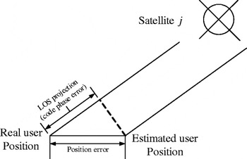
Among other things, a GPS receiver's position error is determined by the pseudorange or code phase errors through a line-of-sight (LOS) projection, as shown in Figure 1.
Relationship between position error and code phase error.

Ignoring all other non-Gaussian error sources such as satellite clock, multipath, hardware bias, etc, the relationship between position error and code phase error can be written as the equation below (Zhao and Akos, Reference Zhao and Akos2011).
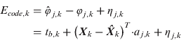
where, the subscript k refers to measurement epoch, E code,k is the code phase error, φ is the code phase measurement, the symbol “^” represents the estimation of a variable, t b,k is the receiver clock bias, X k is the receiver position vector, a j,k is the unit LOS vector from the receiver to the jth satellite, and η is the white Gaussian noise.
Similarly, the carrier frequency error impacts the receiver velocity measurement error:
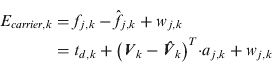
where t d,k is the receiver clock drift and w j,k is the white Gaussian noise.
In a typical GPS receiver, the code phase and carrier frequency measurements in (1) and (2) can be obtained from the tracking loops. The following sections show how to use these measurements so that a vector tracking loop can be formed.
2.1. Process Equation of Vector Tracking Loop
The objective of a GPS receiver is to estimate the receiver position and velocity which are related via a simple linear model:

Where, τ k.k+1 is the discrete time interval, k is the time tag, and Vk is the receiver velocity at epoch k.
The acceleration of the receiver is modeled as a Gaussian distribution white noise, and thus the velocity at epoch k+1 is expressed as below:

The drift of the receiver clock is assumed a constant plus a small white noise. So the clock bias and drift are modelled by equations (5) and (6).


where, r k is the receiver clock drift noise.
The process equation can be established based on equations (3)–(6). The receiver three-dimensional position, velocity, clock bias, and clock drift are the state variables. Equation (7) shows the discrete process equation:
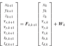
where,
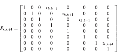
2.2. Measurement Equation of Vector Tracking Loop
Code phase discriminator and carrier frequency discriminator provide noisy code phase error and carrier frequency error when working within their linear range (Kaplan and Hegarty, Reference Kaplan and Hegarty2006). As shown in (1) and (2), the receiver position and velocity are directly affected by the code phases and carrier frequencies observables. Therefore, the outputs of the discriminators are used as the measurements for the integrated Kalman filter as shown in (8):

Where, z code,1,k is the code phase discriminator output of channel 1 at time epoch k, z carrier,1,k is the corresponding carrier frequency discriminator output and the terms in transition matrix H are determined by the following two equations:


Where, a jx,k, a jy,k and a jz,k are the x, y, and z components of the LOS vector pointing from the receiver to the jth satellite at kth epoch, and δx k and δv x,k are the x direction position and velocity errors at kth epoch respectively. It should be noted that the measurements in (8) are not directly related to the system states, i.e. position and velocity. Instead, they are related to their errors. The conventional Kalman filter implementation cannot be directly adopted in this case. A modified Kalman filter described in the next section is used in this study.
3. IMPLEMENTATION OF VECTOR TRACKING LOOP
As mentioned in the previous section, the receiver position, velocity and clock error terms are the Kalman filter states while the position and velocity errors are implicitly embedded in the discriminator outputs. For this reason, an extended Kalman filter (EKF) is applied to process the measurements from the discriminators. For convenience, we adopt the procedure from (Qin et al., Reference Qin, Zhang and Wang1998) and rewrite the discrete equations of EKF as the following:
Prediction:

Estimation:
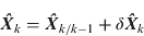
Estimation error calculation:

Kalman gain:

Prediction mean square error:

Estimation mean square error:

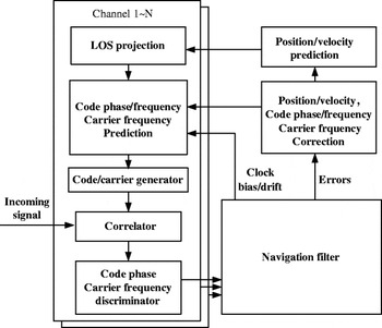
In (11)–(16), f is the one-step transition function and F is the discrete transition matrix, Qk and Rk is the covariance matrices for process and measurement noises, h is the measurement function and H is its discrete matrix. From (8), the outputs of the code phase and carrier frequency discriminators which form the term “δ Zk” in (8), contain the errors of the states (position, velocity, etc). Those errors can be estimated by a standard Kalman filter that employs δ Zk as its measurement. Then, the states are corrected by adding those errors to their predicted values as shown in (12). The flowchart in Figure 2 demonstrates the vector tracking loop (Zhao and Akos, Reference Zhao and Akos2011).
Flowchart of vector tracking loop.

The above described Kalman filter is implemented in Matlab on a software-defined receiver (SDR) (Borre and Akos, Reference Borre, Akos, Bertelsen, Rinder and Jensen2007). This SDR can post-process the recorded GPS intermediate frequency (IF) signal from a hardware GPS signal generator or from live tests. Traditional Costas phase lock loop and code delay lock loop are used to track the carrier and code phases respectively. We shall refer the conventional tracking loop used in SDR as “scalar loop” in the remainder of the paper. Parameters such as bandwidth and damping ratio can be adjusted. Iterative least square method is used to determine the receiver position. The SDR code initially performs acquisition, tracking, and navigation solution processing using the scalar loop approach, and provides the initial variables such as the receiver position, velocity, code phases, carrier frequencies and clock errors to the vector tracking loop. Once the receiver has obtained the ephemeris data and initialized by the scalar loop, tracking is handed over to the vector loop as shown in Figure 2.
4. SIMULATION EXPERIMENT AND RESULTS
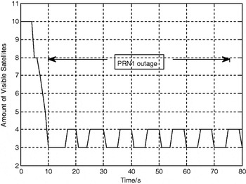
To test the performance of the proposed vector tracking loop, 80 s GPS intermediate frequency signal is recorded from a commercial hardware GPS signal generator. The simulated scenario involves a vehicle making an 8-shaped trajectory in the horizontal plane at a constant speed of 50 m/s. Between 10 s and 80 s, the number of visible satellites varies between 4 and 3 by turning signals from different satellites on and off. The total number of visible satellites throughout the dataset is plotted in Figure 3.
Number of visible satellites versus time.

The signal of PRN1 is blocked from 10 s to 76 s in the dataset. We will focus on the tracking status of PRN1 signal in order to evaluate the performance of vector tracking loop under the low SNR and insufficient visible satellites environment. The SDR scalar loop provides initial tracking loop outputs and the ephemeris before the vector tracking loop starts working. The simulated dataset is also processed by the scalar loop (see parameters listed in Table 1) for comparison purposes.
Scalar loop parameters.

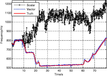
The carrier frequency results from the vector tracking loop are plotted in Figure 4. For comparison, the frequency result from the scalar loop is also plotted in the same figure. Figure 5 exhibits the frequency tracking errors from both scalar loop and vector loop.
PRN1 carrier frequency tracking results.

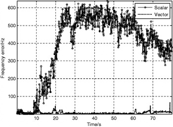
Frequency errors (PRN1).

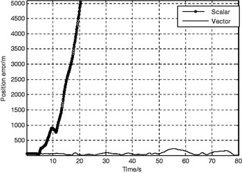
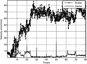
Figures 4 and 5 indicate that when the signal of PRN1 is blocked, the scalar loop cannot estimate the correct carrier frequency due to the independent processing of each channel while the vector loop maintains lock by utilizing outputs from other channels as aid. In the IF signal, PRN1 reappears at 76 s, and the vector loop keeps tracking the signal while the scalar loop is not able to resume tracking once it loses lock. The carrier-to-noise ratio (C/N0) estimations are plotted in Figure 6 to indicate the status of signal tracking for the vector loop and the conventional scalar loop. It shows that after 76 s, the C/N0 estimation from the vector loop increases which indicates that the vector loop successfully tracks the signal, while the scalar loop cannot. From the position and velocity error results in Figures 7 and 8, it is also clear that the vector tracking loop provides more accurate navigation solutions when there are not sufficient available satellites, while the scalar loop fails once the number of visible satellites is below four. It should be noted that, in this scenario, the visible satellite combination contains not the same group of satellites during different time intervals although the total visible number remains no fewer than three through 10 s to 76 s. Therefore, the frequency tracking results of PRN1 and position and velocity results indicate that the vector tracking loop also remains its signal tracking and navigation ability even when different satellite signals disappear and re-appear again.
PRN1 C/N0 estimations.

Position errors.

Velocity errors.

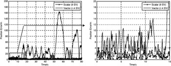
In the meantime, the same scenario is simulated again while there are constantly nine visible satellites throughout the same time period, i.e. PRN1 and the other eight satellites are visible through 10 s to 80 s. For comparison, we use the conventional scalar loop with the same parameters as shown in Table 1 to process this dataset and list the navigation results in Figures 9 and 10.
Position comparison.

Velocity comparison.

The right part of Figure 9 shows the beginning of the dataset when PRN1 is blocked at 10 s in the vector tracking method while in the scalar tracking, there are nine visible satellites. It is clear that, when there are four visible satellites, the vector loop provides comparable position results to the scalar loop although a bit less accurate. However, after the number of visible satellites falls below four, the position results of the vector loop degrades. Figure 10 demonstrates that the velocity results of the vector loop are closer to the scalar loop with nine visible satellites.
5. CONCLUSIONS
This paper presents an implementation of vector loop tracking for GPS receivers operating in an environment where the number of directly visible satellites falls below four. The vector tracking loop is based on an extended Kalman filter design which exploits the relationship between the GPS receiver navigation solutions and the code phase and carrier frequency of the received signal. The paper described the relationship and detailed implementation strategy. A simulation experiment is conducted on a Matlab-based SDR platform to evaluate the post-processing performance of the proposed vector tracking method. The results demonstrate that when there are four or fewer satellites available, the proposed vector tracking loop can maintain tracking on a blocked satellite signal and generate reasonable navigation solutions. And when the signal reappears, the vector loop can detect and track it immediately without re-acquisition. Also, the blockage and reappearance of the other satellites will not affect the tracking status of the blocked signal. Comparing to the scalar loop working under the same scenario but with sufficient amount of visible satellites, the vector loop provides slightly less accurate but almost identical navigation solutions. Thus, comparing with the scalar loop, under the test conditions, the vector loop shows both more robust carrier frequency tracking ability and more accurate navigation solutions.
ACKNOWLEDGMENTS
The authors are very grateful to Professor Dennis Akos within the Department of Aerospace Engineering Sciences, the University of Colorado, USA, for his great support and insightful suggestions on this work.