





1 Introduction
Ubiquitous internal gravity waves are generated in the oceans by tidal flow over bottom topography and by surface storms (Munk & Wunsch Reference Munk and Wunsch1998; Alford Reference Alford2003; Wunsch & Ferrari Reference Wunsch and Ferrari2004). The internal waves transmit energy from generation sites to large distances, and ultimately the energy is converted into small-scale mixing. Internal waves are a major contributor of the energy budget of the oceans, and the mechanism for this contribution can be better understood through the energy flux field. In this paper, we examine the baroclinic energy flux
 $\boldsymbol{J}(x,z,t)$
,
 $$\begin{eqnarray}\displaystyle \boldsymbol{J}=p\,\boldsymbol{v}, & & \displaystyle\end{eqnarray}$$
in the presence of a stable background density stratification with a buoyancy frequency profile
 $N(z)$
, where
 $p(x,z,t)$
is the pressure perturbation from the background hydrostatic pressure field, and
 $\boldsymbol{v}(x,z,t)$
is the velocity perturbation from the background velocity flow field. Determining the energy flux requires the simultaneous measurement of both the pressure and velocity perturbation fields. In numerical investigations of internal waves, these fields are computed (Lamb Reference Lamb2004; Niwa & Hibiya Reference Niwa and Hibiya2004; King, Zhang & Swinney Reference King, Zhang and Swinney2009, Reference King, Zhang and Swinney2010; Zilberman et al.
Reference Zilberman, Becker, Merrifield and Carter2009; Gayen & Sarkar Reference Gayen and Sarkar2010, Reference Gayen and Sarkar2011; Rapaka, Gayen & Sarkar Reference Rapaka, Gayen and Sarkar2013), enabling a direct calculation of the energy flux. However, in laboratory and field studies, simultaneous measurements of the velocity and pressure perturbation fields are usually not possible.
Laboratory observations of internal waves have been made by particle image velocimetry (PIV) (Echeverri et al. Reference Echeverri, Flynn, Winters and Peacock2009; King et al. Reference King, Zhang and Swinney2009, Reference King, Zhang and Swinney2010; Paoletti, Drake & Swinney Reference Paoletti, Drake and Swinney2014), synthetic schlieren (Sutherland et al. Reference Sutherland, Dalziel, Hughes and Linden1999; Dalziel, Hughes & Sutherland Reference Dalziel, Hughes and Sutherland2000; Clark & Sutherland Reference Clark and Sutherland2010; Allshouse et al. Reference Allshouse, Lee, Morrison and Swinney2016) and light attenuation (Dossmann et al. Reference Dossmann, Rosevear, Griffiths, Hogg, Hughes and Copeland2016). In PIV, neutrally buoyant particles scatter incident laser light, and movies of the scattered light field yield the time-varying velocity field. In the schlieren method, a patterned mask is placed behind a tank that contains the internal waves, and the time-varying distorted image formed by light transmitted through the tank in the transverse direction gives the time-dependent density perturbation field (Sutherland et al. Reference Sutherland, Dalziel, Hughes and Linden1999; Dalziel et al. Reference Dalziel, Hughes and Sutherland2000). The light attenuation technique uses dye intensity that varies with depth and moves with the fluid to measure the density field as a function of time (Dossmann et al. Reference Dossmann, Rosevear, Griffiths, Hogg, Hughes and Copeland2016). These experimental techniques yield the velocity field in the case of PIV and the density perturbation field in the case of synthetic schlieren and light attenuation measurements. No experimental technique directly yields the pressure perturbation field needed for the energy flux calculation.
Given the importance of the energy flux and the far-field radiated power obtained by integrating the flux, multiple efforts have been made to calculate the energy flux from experimental measurements. One method assumed a constant buoyancy frequency and calculated the energy flux (averaged over a tidal period) given only the streamfunction, thus eliminating the need to measure the pressure perturbation field (Balmforth, Ierley & Young Reference Balmforth, Ierley and Young2002). The streamfunction method was subsequently extended to a buoyancy frequency varying exponentially with depth (Llewellyn Smith & Young Reference Llewellyn Smith and Young2003; Lee et al. Reference Lee, Paoletti, Swinney and Morrison2014). Another method applied the polarization relations to density perturbation data to obtain estimates for the velocity and pressure perturbation amplitudes (Clark & Sutherland Reference Clark and Sutherland2010). This method provided the energy flux time averaged over a tidal period for a monochromatic plane wave, which is not representative of the complex ocean internal wave fields, which have many natural frequencies and spatially varying wave packets. Finally, an ocean observation analysis technique calculated the pressure perturbation field for measured density profiles, assuming a hydrostatic pressure field; this together with simultaneous velocity measurements allowed the calculation of the energy flux field (Nash, Alford & Kunze Reference Nash, Alford and Kunze2005). This method assumed that the contribution of dynamic pressure is negligible, which is often not the case in experiments and in high velocity events in the ocean.
The methods presented here for obtaining the instantaneous energy flux from laboratory and field data differ from previous methods that determined the time-averaged energy flux or a global energy conversion rate. Recently, Allshouse et al. (Reference Allshouse, Lee, Morrison and Swinney2016) developed a Green’s function method was used to calculate the instantaneous energy flux field from a density perturbation field for a fluid with constant buoyancy frequency, where the buoyancy frequency is
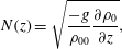 $$\begin{eqnarray}\displaystyle N(z)=\sqrt{\frac{-g}{\unicode[STIX]{x1D70C}_{00}}\frac{\unicode[STIX]{x2202}\unicode[STIX]{x1D70C}_{0}}{\unicode[STIX]{x2202}z}}, & & \displaystyle\end{eqnarray}$$
where
 $\unicode[STIX]{x1D70C}_{00}$
is a reference density taken here to be
 $1000~\text{kg}~\text{m}^{-3}$
and
 $\unicode[STIX]{x1D70C}_{0}(z)$
is the unperturbed, background density profile. However, in the oceans
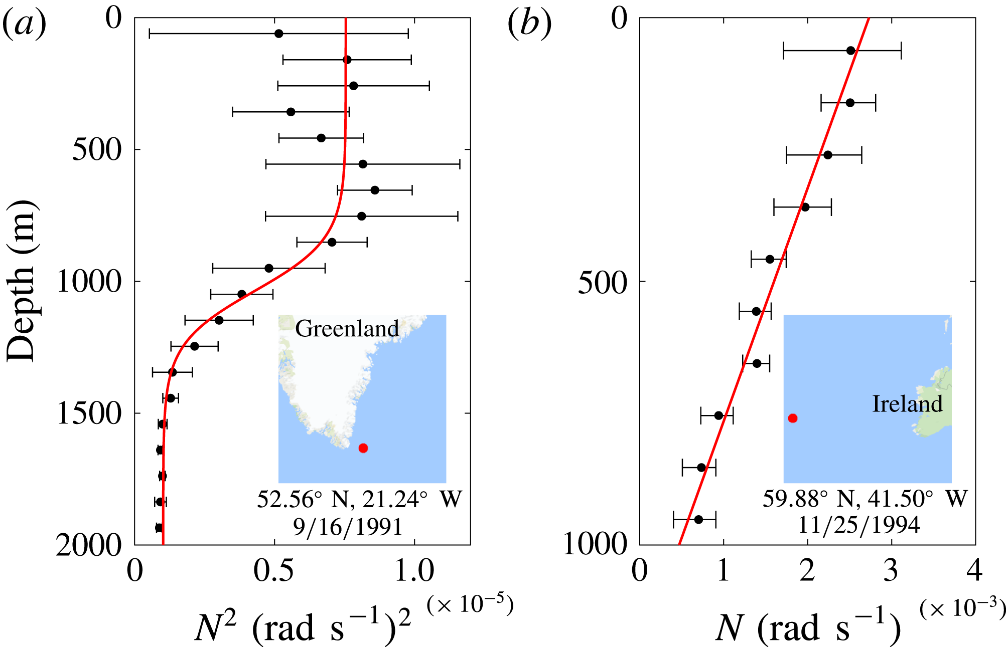
 $N$
varies significantly with depth, as figure 1 illustrates with data from two locations in the North Atlantic.
Two buoyancy frequency profiles computed from the World Ocean Circulation Experiment data sets by the method of King et al. (Reference King, Stone, Zhang, Gerkema, Marder, Scott and Swinney2012). (a) A measured buoyancy frequency squared profile (black dots) fit to a tanh profile (red). (b) A measured buoyancy frequency profile (black dots) fit to a linear profile (red). The insets show regions
 $1000~\text{km}\times 1000~\text{km}$
that contain the locations (red dots) where the measurements were made. The mean buoyancy frequency (squared for (a)) of bins of stratification measurements is plotted as a function of depth (black dots) with error bars representing two standard deviations from the mean.
Recognizing the strength of the Green’s function method, we extend that method to accommodate a profile with
 $N$
varying linearly with
 $z$
, and a tanh
 $N^{2}$
profile. These two profiles are selected due to their mathematical properties and their presence in ocean stratifications. The
 $\tanh N^{2}$
profile is often a good approximation in the ocean where two nearly constant buoyancy frequency zones are separated by a transition region, as figure 1(a) illustrates. The linear
 $N$
profile can occur in the ocean when there is no narrow region with a rapid change in
 $N(z)$
, as illustrated in figure 1(b).
Many buoyancy frequency profiles cannot be adequately approximated by either a linear
 $N$
or a tanh
 $N^{2}$
profile as in figure 1. Other examples of buoyancy frequency profiles are presented in figure 5 of King et al. (Reference King, Stone, Zhang, Gerkema, Marder, Scott and Swinney2012). The general
 $N(z)$
case must be treated separately from the linear
 $N$
or a tanh
 $N^{2}$
cases. Hence we present a numerical method for computing the instantaneous energy flux field solely from a density perturbation field that can have an arbitrary
 $N(z)$
profile.
The present work provides a method for the calculation of the instantaneous energy flux field from density perturbation data. Our method provides the instantaneous rather than time-averaged energy flux field. Thus the resultant energy flux and integrated far-field power include all spectral components, while previous methods provided only the global conversion rates or monochromatic results. Application of this method to experimental systems requires the density perturbation field, obtained for example by synthetic schlieren or light attenuation measurements. Application to ocean observations will require a time-varying density perturbation field that can be measured using, for example, a Fast-CTD (Conductivity, Temperature and Density) system (Pinkel, Buijsman & Klymak Reference Pinkel, Buijsman and Klymak2012) or a moving wirewalker (Pinkel et al. Reference Pinkel, Goldin, Smith, Sun, Aja, Bui and Hughen2011).
The paper is organized as follows. An outline of our method for obtaining the energy flux from the density perturbation field in a tanh
 $N^{2}$
and linear
 $N$
stratification is presented in § 2. This method is then verified with numerical simulations in § 3. A finite difference method for calculating the energy flux for an arbitrary buoyancy frequency profile is presented in § 4, and is applied to an ocean-inspired stratification. Then we present in § 5 scaling arguments for the errors in the velocity components and the pressure perturbation due to nonlinearities, since the method assumes linearity, and these error scalings are verified using parameter sweeps with the numerical simulations. Lastly, conclusions and potential applications of this work are presented in § 6.
2 Theoretical development
The general equations for the method are presented in § 2.1, which builds on the theoretical foundation presented in Allshouse et al. (Reference Allshouse, Lee, Morrison and Swinney2016). The equations provide the velocity perturbation components
 $u(x,z,t)$
and
 $w(x,z,t)$
as a function of the density perturbation field
 $\unicode[STIX]{x1D70C}(x,z,t)$
and provide a functional relationship between the density and pressure perturbation fields. For an analytic tanh
 $N^{2}(z)$
and a linear
 $N(z)$
, we calculate the Green’s function in §§ 2.2 and 2.3, respectively.
2.1 Generalities
Our goal of obtaining the energy flux (1.1) from the density perturbation field alone requires calculating the pressure perturbation and components of the velocity perturbation from the density perturbation field. The details of these calculations were given in Allshouse et al. (Reference Allshouse, Lee, Morrison and Swinney2016) for a uniform
 $N$
profile, but here we present a condensed version of the pressure perturbation calculation, which is needed for the calculations for the tanh
 $N^{2}$
and linear
 $N$
profiles.
We begin with the linearized two-dimensional Euler equations for perturbation about a hydrostatic background, neglecting rotation,
 $$\begin{eqnarray}\displaystyle \frac{\unicode[STIX]{x2202}u}{\unicode[STIX]{x2202}t}=-\frac{1}{\unicode[STIX]{x1D70C}_{0}}\frac{\unicode[STIX]{x2202}p}{\unicode[STIX]{x2202}x},\quad \frac{\unicode[STIX]{x2202}w}{\unicode[STIX]{x2202}t}=-\frac{1}{\unicode[STIX]{x1D70C}_{0}}\frac{\unicode[STIX]{x2202}p}{\unicode[STIX]{x2202}z}-\frac{\unicode[STIX]{x1D70C}}{\unicode[STIX]{x1D70C}_{0}}g, & & \displaystyle\end{eqnarray}$$
 $$\begin{eqnarray}\displaystyle \frac{\unicode[STIX]{x2202}\unicode[STIX]{x1D70C}}{\unicode[STIX]{x2202}t}=\frac{N^{2}\,\unicode[STIX]{x1D70C}_{0}}{g}w,\quad \frac{\unicode[STIX]{x2202}u}{\unicode[STIX]{x2202}x}+\frac{\unicode[STIX]{x2202}w}{\unicode[STIX]{x2202}z}=0, & & \displaystyle\end{eqnarray}$$
where
 $u$
and
 $w$
are the horizontal and vertical components of the velocity perturbation, respectively,
 $p$
is the pressure perturbation,
 $\unicode[STIX]{x1D70C}$
is the density perturbation,
 $\unicode[STIX]{x1D70C}_{0}$
is the hydrostatic background density profile and
 $N$
is the buoyancy frequency. The total pressure
 $p_{T}$
and density
 $\unicode[STIX]{x1D70C}_{T}$
are separated into their respective background and perturbation quantities by
 $p_{T}=p_{0}(z)+p(x,z,t)$
and
 $\unicode[STIX]{x1D70C}_{T}=\unicode[STIX]{x1D70C}_{0}(z)+\unicode[STIX]{x1D70C}(x,z,t)$
for this linearization. By manipulating (2.1) and (2.2) we obtain an equation for the pressure perturbation in terms of the density perturbation,
 $$\begin{eqnarray}\displaystyle \frac{\unicode[STIX]{x2202}^{2}p}{\unicode[STIX]{x2202}x^{2}}+\frac{\unicode[STIX]{x2202}^{2}p}{\unicode[STIX]{x2202}z^{2}}+\frac{N^{2}}{g}\frac{\unicode[STIX]{x2202}p}{\unicode[STIX]{x2202}z}=-N^{2}\unicode[STIX]{x1D70C}-g\frac{\unicode[STIX]{x2202}\unicode[STIX]{x1D70C}}{\unicode[STIX]{x2202}z}. & & \displaystyle\end{eqnarray}$$
Because (2.3) is valid at any given instant in time, explicit time dependence is omitted in (2.3) and in the following derivations.
Equation (2.3) is solved for
 $p$
assuming
 $\unicode[STIX]{x1D70C}$
is given. Equation (2.3) is brought into a convenient form by applying the following transformation:
 $$\begin{eqnarray}\displaystyle p(x,z)=s(x,z)\,T(z), & & \displaystyle\end{eqnarray}$$
where
 $$\begin{eqnarray}\displaystyle T(z)=\exp \left[-\frac{1}{2g}\int ^{z}\text{d}z^{\prime }N^{2}(z^{\prime })\right], & & \displaystyle\end{eqnarray}$$
and then Fourier expanding in
 $x$
to obtain
 $$\begin{eqnarray}\displaystyle \frac{\text{d}^{2}S}{\text{d}z^{2}}-\left(k^{2}+\frac{N}{g}\frac{\text{d}N}{\text{d}z}+\frac{N^{4}}{4\,g^{2}}\right)S=-R. & & \displaystyle\end{eqnarray}$$
Here
 $R(z;k)$
and
 $S(z;k)$
denote the Fourier components of
 $$\begin{eqnarray}\displaystyle r(x,z)=\frac{1}{T(z)}\left(N^{2}\unicode[STIX]{x1D70C}+g\frac{\unicode[STIX]{x2202}\unicode[STIX]{x1D70C}}{\unicode[STIX]{x2202}z}\right) & & \displaystyle\end{eqnarray}$$
and
 $s(x,z)$
, respectively.
We solve (2.6) for
 $S$
given
 $R$
by obtaining the Green’s function for the Fourier components, which satisfies
 $$\begin{eqnarray}\displaystyle \frac{\text{d}^{2}}{\text{d}z^{2}}G(z,z^{\prime };k)-\left(k^{2}+\frac{N}{g}\frac{\text{d}N}{\text{d}z}+\frac{N^{4}}{4g^{2}}\right)G(z,z^{\prime };k)=0,\quad z\neq z^{\prime }, & & \displaystyle\end{eqnarray}$$
with a no-flux condition in the
 $z$
direction at the bottom (
 $z=0$
) and top (
 $z=h$
) of the domain,
 $$\begin{eqnarray}\displaystyle \left.\left(\frac{\text{d}G}{\text{d}z}-\frac{N^{2}}{2g}G\right)\right|_{z=0,\,h}=0, & & \displaystyle\end{eqnarray}$$
and the Green’s function matching conditions,
 $$\begin{eqnarray}\displaystyle G^{+}(z^{\prime }) & = & \displaystyle G^{-}(z^{\prime })\end{eqnarray}$$
 $$\begin{eqnarray}\displaystyle \frac{\text{d}G^{+}}{\text{d}z}(z^{\prime }) & = & \displaystyle \frac{\text{d}G^{-}}{\text{d}z}(z^{\prime })+1.\end{eqnarray}$$
Here,
 $G^{+}$
and
 $G^{-}$
indicate the two parts of
 $G$
for
 $z\geqslant z^{\prime }$
and
 $z\leqslant z^{\prime }$
, respectively, where
 $z$
is the location of evaluation and
 $z^{\prime }$
is the location of the source. Thus, given profiles for the buoyancy frequency
 $N$
and source term
 $r$
, the pressure perturbation is given by the following expression:
 $$\begin{eqnarray}\displaystyle p(x,z)=\text{Re}\left\{-\frac{2}{l}\,T(z)\mathop{\sum }_{k}\text{e}^{-\text{i}kx}\int _{0}^{h}\text{d}z^{\prime }\,G(z,z^{\prime };k)\,\int _{0}^{l}\text{d}x^{\prime }\,r(x^{\prime },z^{\prime })\,\text{e}^{\text{i}kx^{\prime }}\right\}, & & \displaystyle\end{eqnarray}$$
where
 $k=2\unicode[STIX]{x03C0}n/l$
,
 $l$
is the width of the system, and
 $n$
is a positive integer.
Next, we obtain the components of the velocity perturbation. The vertical component follows by inverting (2.2a ), which yields
 $$\begin{eqnarray}\displaystyle w=\frac{g}{N^{2}\,\unicode[STIX]{x1D70C}_{0}}\frac{\unicode[STIX]{x2202}\unicode[STIX]{x1D70C}}{\unicode[STIX]{x2202}t}. & & \displaystyle\end{eqnarray}$$
The horizontal component is obtained by using the vertical velocity perturbation (2.13) and the incompressibility condition, (2.2b ), which gives the differential equation
 $$\begin{eqnarray}\displaystyle \frac{\unicode[STIX]{x2202}u}{\unicode[STIX]{x2202}x}=-\frac{\unicode[STIX]{x2202}}{\unicode[STIX]{x2202}z}\left(\frac{g}{N^{2}\unicode[STIX]{x1D70C}_{0}}\frac{\unicode[STIX]{x2202}\unicode[STIX]{x1D70C}}{\unicode[STIX]{x2202}t}\right), & & \displaystyle\end{eqnarray}$$
which can be integrated along horizontal slices of data to get
 $u$
. This horizontal integration requires an integration constant at each horizontal slice of the system. It is possible to assume the point along the horizontal slice with negligible change in density corresponds to a point of negligible horizontal velocity. In experiments, it is possible to find these regions of negligible flow outside the wave beams, but this may not be straightforward in ocean data.
The forms of (2.12), (2.13) and (2.14) are valid for a general stratification, so it is possible to compute all the necessary expressions for the energy flux from
 $\unicode[STIX]{x1D70C}$
alone. However, to calculate analytically the Green’s function for (2.8), it is necessary that the functional form of the buoyancy frequency profile be specified. Allshouse et al. (Reference Allshouse, Lee, Morrison and Swinney2016) investigated the particular case where the buoyancy frequency is constant resulting in a Green’s function that is exponential. In § 2.2 we present the calculations for obtaining the pressure perturbation for the tanh
 $N^{2}$
profile, and in § 2.3 we present the analogous calculation for the linear
 $N$
profile.
2.2 The tanh profile
The buoyancy frequency profile we assume in this section is given by
 $$\begin{eqnarray}\displaystyle N^{2}(z) & = & \displaystyle \frac{N_{1}^{2}+N_{2}^{2}}{2}+\frac{N_{2}^{2}-N_{1}^{2}}{2}\tanh (\unicode[STIX]{x1D6FC}(z-z_{t}))\end{eqnarray}$$
 $$\begin{eqnarray}\displaystyle & \equiv & \displaystyle \unicode[STIX]{x1D702}_{+}+\unicode[STIX]{x1D702}_{-}\tanh (\unicode[STIX]{x1D6FC}(z-z_{t})),\end{eqnarray}$$
because this gives a convenient form for
 $N\,\text{d}N/\text{d}z$
. Here
 $\unicode[STIX]{x1D6FC}$
controls the transition width between the two buoyancy frequency values
 $N_{1}$
and
 $N_{2}$
, and
 $z_{t}$
is the midpoint of the transition. For large
 $\unicode[STIX]{x1D6FC}$
, equation (2.16) approximates a two-layer
 $N^{2}$
profile, which we will investigate in § 3.2.
With the buoyancy frequency profile in (2.16), we can estimate the contributions of each of the terms in (2.8). For experimental systems, we can use the orders of magnitude
 $N\sim 10^{-1}{-}10^{0}~\text{rad}~\text{s}^{-1}$
,
 $l\sim 10^{-1}{-}10^{0}$
m and
 $\text{d}N/\text{d}z\sim 10^{0}{-}10^{2}~\text{rad}~\text{m}^{-1}~\text{s}^{-1}$
, which are based on experimental internal wave beams (Mathur & Peacock Reference Mathur and Peacock2009; Paoletti & Swinney Reference Paoletti and Swinney2012; Ghaemsaidi et al.
Reference Ghaemsaidi, Joubaud, Dauxois, Odier and Peacock2016). With these estimates, it can be shown that
 $k^{2}\sim (10^{1}{-}10^{3})n^{2}~\text{m}^{-2}$
and
 $N^{4}/4g^{2}\sim 10^{-6}{-}10^{-2}~\text{m}^{-2}$
. In regions where
 $N$
changes rapidly,
 $(N/g)(\text{d}N/\text{d}z)\sim 10^{1}~\text{m}^{-2}$
, which means
 $k^{2}>(N/g)(\text{d}N/\text{d}z)\gg N^{4}/4g^{2}$
. In regions where
 $N$
changes slowly,
 $(N/g)(\text{d}N/\text{d}z)$
can be similar to or even smaller than
 $N^{4}/4g^{2}$
, which means, for any
 $n$
,
 $k^{2}\gg N^{4}/4g^{2}\sim (N/g)(\text{d}N/\text{d}z)$
. However, to simplify the calculations, we simply drop
 $N^{4}/4g^{2}$
for all regions. This provides a uniformly good approximation to the ‘potential term’ in (2.8), without the need to represent and solve the equation in a piecewise manner for the two types of regions, which would complicate the calculations. Similar arguments could be made for observational data when using the orders of magnitude
 $N\sim 10^{-4}{-}10^{-2}~\text{rad}~\text{s}^{-1}$
,
 $l\sim 10^{2}{-}10^{3}$
m, and
 $\text{d}N/\text{d}z\sim 0{-}10^{-4}~\text{rad}~\text{m}^{-1}~\text{s}^{-1}$
, based on Gerkema, Lam & Maas (Reference Gerkema, Lam and Maas2004) and Martin, Rudnick & Pinkel (Reference Martin, Rudnick and Pinkel2006).
Upon dropping
 $N^{4}/4g^{2}$
in (2.8), and substituting the stratification of (2.16), the Green’s function equation (2.8) becomes
 $$\begin{eqnarray}\displaystyle \frac{\unicode[STIX]{x2202}^{2}}{\unicode[STIX]{x2202}z^{2}}G(z,z^{\prime };k)-\left(k^{2}+\frac{\unicode[STIX]{x1D6FC}\,\unicode[STIX]{x1D702}_{-}}{2\,g}\operatorname{sech}^{2}(\unicode[STIX]{x1D6FC}(z-z_{t}))\right)G(z,z^{\prime };k)=0,\quad z\neq z^{\prime }. & & \displaystyle\end{eqnarray}$$
Equation (2.17) is of the form of a well-studied time-independent Schrödinger equation (e.g. Epstein Reference Epstein1930; Pöshl & Teller Reference Pöshl and Teller1933; Lekner Reference Lekner2007).
With the dimensionless coordinate transformation
 $$\begin{eqnarray}\displaystyle z=z_{t}+\frac{1}{\unicode[STIX]{x1D6FC}}\tanh ^{-1}y, & & \displaystyle\end{eqnarray}$$
equation (2.17) becomes
 $$\begin{eqnarray}\displaystyle (1-y^{2})\frac{\text{d}^{2}\bar{G}}{\text{d}y^{2}}-2\,y\frac{\text{d}\bar{G}}{\text{d}y}+\left(\unicode[STIX]{x1D708}(\unicode[STIX]{x1D708}+1)-\frac{\unicode[STIX]{x1D707}^{2}}{1-y^{2}}\right)\bar{G}=0,\quad y\neq y^{\prime }, & & \displaystyle\end{eqnarray}$$
where the dimensionless Green’s function
 $\bar{G}$
is given by
 $$\begin{eqnarray}\displaystyle G(z(y))=\frac{1}{\unicode[STIX]{x1D6FC}}\bar{G}(y), & & \displaystyle\end{eqnarray}$$
and the parameters
 $\unicode[STIX]{x1D708}$
and
 $\unicode[STIX]{x1D707}$
are given by
 $$\begin{eqnarray}\displaystyle \unicode[STIX]{x1D708}_{\pm }=-\frac{1}{2}\pm \frac{1}{2}\sqrt{1-\frac{2\,\unicode[STIX]{x1D702}_{-}}{\unicode[STIX]{x1D6FC}\,g}},\quad \unicode[STIX]{x1D707}=\frac{k}{\unicode[STIX]{x1D6FC}}. & & \displaystyle\end{eqnarray}$$
Thus the transformation takes (2.17) into the associated Legendre equation (2.19), which has the two linearly independent solutions
 $P_{\unicode[STIX]{x1D708}}^{\unicode[STIX]{x1D707}}(y)$
and
 $Q_{\unicode[STIX]{x1D708}}^{\unicode[STIX]{x1D707}}(y)$
, the associated Legendre functions of the first and second kind, respectively. From the definition of the Legendre functions, both
 $\unicode[STIX]{x1D708}_{+}$
and
 $\unicode[STIX]{x1D708}_{-}$
will produce the same result. We use
 $\unicode[STIX]{x1D708}_{+}$
throughout our calculations, but will represent this as
 $\unicode[STIX]{x1D708}$
for brevity. Then, solving (2.19) with the boundary conditions (2.9) and the matching conditions (2.10) and (2.11) gives the Green’s function,
 $$\begin{eqnarray}\displaystyle \bar{G}(y,y^{\prime })=\frac{1}{D_{T}\,W}\left\{\begin{array}{@{}ll@{}}(\unicode[STIX]{x1D6F7}_{2}P_{\unicode[STIX]{x1D708}}^{\unicode[STIX]{x1D707}}(y^{\prime })+\unicode[STIX]{x1D6F1}_{2}Q_{\unicode[STIX]{x1D708}}^{\unicode[STIX]{x1D707}}(y^{\prime }))(\unicode[STIX]{x1D6F7}_{1}P_{\unicode[STIX]{x1D708}}^{\unicode[STIX]{x1D707}}(y)+\unicode[STIX]{x1D6F1}_{1}Q_{\unicode[STIX]{x1D708}}^{\unicode[STIX]{x1D707}}(y)),\quad & y<y^{\prime }\\ (\unicode[STIX]{x1D6F7}_{1}P_{\unicode[STIX]{x1D708}}^{\unicode[STIX]{x1D707}}(y^{\prime })+\unicode[STIX]{x1D6F1}_{1}Q_{\unicode[STIX]{x1D708}}^{\unicode[STIX]{x1D707}}(y^{\prime }))(\unicode[STIX]{x1D6F7}_{2}P_{\unicode[STIX]{x1D708}}^{\unicode[STIX]{x1D707}}(y)+\unicode[STIX]{x1D6F1}_{2}Q_{\unicode[STIX]{x1D708}}^{\unicode[STIX]{x1D707}}(y)),\quad & y>y^{\prime }.\end{array}\right. & & \displaystyle\end{eqnarray}$$
Here
 $$\begin{eqnarray}\displaystyle D_{T}=-\left|\begin{array}{@{}cc@{}}\unicode[STIX]{x1D6F1}_{1} & \unicode[STIX]{x1D6F1}_{2}\\ \unicode[STIX]{x1D6F7}_{1} & \unicode[STIX]{x1D6F7}_{2}\end{array}\right|,\quad W=2^{2\unicode[STIX]{x1D707}}\frac{\displaystyle \unicode[STIX]{x0393}\left(\frac{\unicode[STIX]{x1D708}+\unicode[STIX]{x1D707}+2}{2}\right)\unicode[STIX]{x0393}\left(\frac{\unicode[STIX]{x1D708}+\unicode[STIX]{x1D707}+1}{2}\right)}{\displaystyle \unicode[STIX]{x0393}\left(\frac{\unicode[STIX]{x1D708}-\unicode[STIX]{x1D707}+2}{2}\right)\unicode[STIX]{x0393}\left(\frac{\unicode[STIX]{x1D708}-\unicode[STIX]{x1D707}+1}{2}\right)}, & & \displaystyle\end{eqnarray}$$
 $$\begin{eqnarray}\displaystyle \unicode[STIX]{x1D6F1}_{1,2}=\frac{\text{d}P_{\unicode[STIX]{x1D708}}^{\unicode[STIX]{x1D707}}}{\text{d}y}(y_{0,h})-\frac{N_{1,2}^{2}}{2\,g\,(1-y_{0,h}^{2})}P_{\unicode[STIX]{x1D708}}^{\unicode[STIX]{x1D707}}(y_{0,h}), & & \displaystyle\end{eqnarray}$$
 $$\begin{eqnarray}\displaystyle \unicode[STIX]{x1D6F7}_{1,2}=-\frac{\text{d}Q_{\unicode[STIX]{x1D708}}^{\unicode[STIX]{x1D707}}}{\text{d}y}(y_{0,h})+\frac{N_{1,2}^{2}}{2\,g\,(1-y_{0,h}^{2})}Q_{\unicode[STIX]{x1D708}}^{\unicode[STIX]{x1D707}}(y_{0,h}). & & \displaystyle\end{eqnarray}$$
The quantities
 $y_{0,h}$
represent
 $y(z=0)$
and
 $y(z=h)$
, respectively. Note, the transformation factor
 $T(z)$
for this case is given by
 $$\begin{eqnarray}\displaystyle T(z)=\left\{\frac{\cosh [\unicode[STIX]{x1D6FC}(z_{0}-z_{t})]}{\cosh [\unicode[STIX]{x1D6FC}(z-z_{t})]}\right\}^{\unicode[STIX]{x1D702}_{-}/(2\,\unicode[STIX]{x1D6FC}\,g)}\exp \left[\frac{\unicode[STIX]{x1D702}_{+}(z_{0}-z)}{2\,g}\right]. & & \displaystyle\end{eqnarray}$$
Here,
 $z_{0}$
is the integration constant that comes from the integral in (2.5). For further information on the numerical calculation of the Green’s function see the Supplementary materials (https://doi.org/10.1017/jfm.2018.699).
2.3 The linear profile
The calculations for the linear
 $N$
profile are similar to those of § 2.2, so we only highlight the important differences. The linear profile for the buoyancy frequency is given by
 $$\begin{eqnarray}\displaystyle N(z)=(z-z_{t})\frac{\text{d}N}{\text{d}z}\equiv (z-z_{t})N^{\prime }, & & \displaystyle\end{eqnarray}$$
where
 $z_{t}$
is now the location where the buoyancy frequency becomes zero, and
 $N^{\prime }$
is the constant gradient of
 $N(z)$
. Substituting (2.27) into (2.8), we again neglect
 $N^{4}/4g^{2}$
relative to
 $k^{2}$
and
 $(N/g)(\text{d}N/\text{d}z)$
in (2.8) due to the same scaling argument presented in § 2.2. Thus for the linear
 $N$
profile, instead of (2.17) we obtain
 $$\begin{eqnarray}\displaystyle \frac{\unicode[STIX]{x2202}^{2}}{\unicode[STIX]{x2202}z^{2}}G(z,z^{\prime };k)-\left(k^{2}+(N^{\prime })^{2}\frac{(z-z_{t})}{g}\right)G(z,z^{\prime };k)=0,\quad z\neq z^{\prime }. & & \displaystyle\end{eqnarray}$$
With the coordinate transformation
 $$\begin{eqnarray}\displaystyle z=z_{t}-g\,k^{2}(N^{\prime })^{-2}+g^{1/3}(N^{\prime })^{-2/3}\,y, & & \displaystyle\end{eqnarray}$$
where once again
 $y$
is a dimensionless coordinate variable, equation (2.28) becomes
 $$\begin{eqnarray}\displaystyle \frac{\text{d}^{2}}{\text{d}y^{2}}\bar{G}(y)-y\,\bar{G}(y)=0,\quad y\neq y^{\prime }, & & \displaystyle\end{eqnarray}$$
which is the Airy equation with the two independent solutions
 $Ai(y)$
and
 $Bi(y)$
, the Airy functions of the first and second kind, respectively. Then, the dimensionless Green’s function is given by
 $$\begin{eqnarray}\displaystyle \bar{G}(y,y^{\prime })=\frac{\unicode[STIX]{x03C0}}{D_{L}}\left\{\begin{array}{@{}ll@{}}\left(\unicode[STIX]{x1D6FD}_{2}Ai(y^{\prime })+\unicode[STIX]{x1D6FC}_{2}Bi(y^{\prime })\right)\left(\unicode[STIX]{x1D6FD}_{1}Ai(y)+\unicode[STIX]{x1D6FC}_{1}Bi(y)\right),\quad & y<y^{\prime }\\ \left(\unicode[STIX]{x1D6FD}_{1}Ai(y^{\prime })+\unicode[STIX]{x1D6FC}_{1}Bi(y^{\prime })\right)\left(\unicode[STIX]{x1D6FD}_{2}Ai(y)+\unicode[STIX]{x1D6FC}_{2}Bi(y)\right),\quad & y>y^{\prime },\end{array}\right. & & \displaystyle\end{eqnarray}$$
which when given dimensions becomes
 $$\begin{eqnarray}\displaystyle G(z(y))=g^{1/3}(N^{\prime })^{-2/3}\bar{G}(y). & & \displaystyle\end{eqnarray}$$
Here
 $$\begin{eqnarray}\displaystyle & \displaystyle D_{L}=-\left|\begin{array}{@{}cc@{}}\unicode[STIX]{x1D6FC}_{1} & \unicode[STIX]{x1D6FC}_{2}\\ \unicode[STIX]{x1D6FD}_{1} & \unicode[STIX]{x1D6FD}_{2}\end{array}\right|, & \displaystyle\end{eqnarray}$$
 $$\begin{eqnarray}\displaystyle & \displaystyle \unicode[STIX]{x1D6FC}_{1,2}=\frac{\text{d}Ai}{\text{d}y}(y_{0,h})-\frac{1}{2}\,g^{-2/3}(N^{\prime })^{4/3}(z_{0,h}-z_{t})^{2}Ai(y_{0,h}), & \displaystyle\end{eqnarray}$$
 $$\begin{eqnarray}\displaystyle & \displaystyle \unicode[STIX]{x1D6FD}_{1,2}=-\frac{\text{d}Bi}{\text{d}y}(y_{0,h})+\frac{1}{2}\,g^{-2/3}(N^{\prime })^{4/3}(z_{0,h}-z_{t})^{2}Bi(y_{0,h}), & \displaystyle\end{eqnarray}$$
where
 $z_{0}$
and
 $z_{h}$
are the coordinates of the bottom and top of the domain, respectively, and
 $y_{0}$
and
 $y_{h}$
are the corresponding transformed coordinates. The transformation factor
 $T(z)$
in this case is given by
 $$\begin{eqnarray}\displaystyle T(z)=\exp \left\{\frac{(N^{\prime })^{3}}{6\,g}[(z_{0}-z_{t})^{3}-(z-z_{t})^{3}]\right\}. & & \displaystyle\end{eqnarray}$$
Here, as before,
 $z_{0}$
is the integration constant that comes from the integral in (2.5).
3 Verification of Green’s function analysis
To verify the Green’s function analysis in § 2, we compare those predictions with results for the energy flux obtained from direct numerical simulations of the Navier–Stokes equations. The simulations are described in § 3.1. The simulated velocity perturbation, pressure perturbation and energy flux fields of internal waves in a stratified fluid are compared with the predictions from the analyses for a tanh
 $N^{2}$
profile in § 3.2 and for a linear
 $N$
profile in § 3.3.
3.1 Simulation of the density perturbation field
To verify the Green’s function method, we perform direct numerical simulations of the Navier–Stokes equations in the Boussinesq approximation. These simulations provide the density perturbation field needed to calculate the velocity perturbation, pressure perturbation and energy flux fields. The simulations use the CDP-2.4 algorithm, which is a finite volume solver that implements a fractional-step time-marching scheme (Ham & Iaccarino Reference Ham and Iaccarino2004; Mahesh, Constantinescu & Moin Reference Mahesh, Constantinescu and Moin2004). This code has previously been used to simulate internal waves and has been validated with experiments (King et al. Reference King, Zhang and Swinney2009; Dettner, Paoletti & Swinney Reference Dettner, Paoletti and Swinney2013; Lee et al. Reference Lee, Paoletti, Swinney and Morrison2014; Paoletti et al. Reference Paoletti, Drake and Swinney2014; Zhang & Swinney Reference Zhang and Swinney2014; Allshouse et al. Reference Allshouse, Lee, Morrison and Swinney2016).
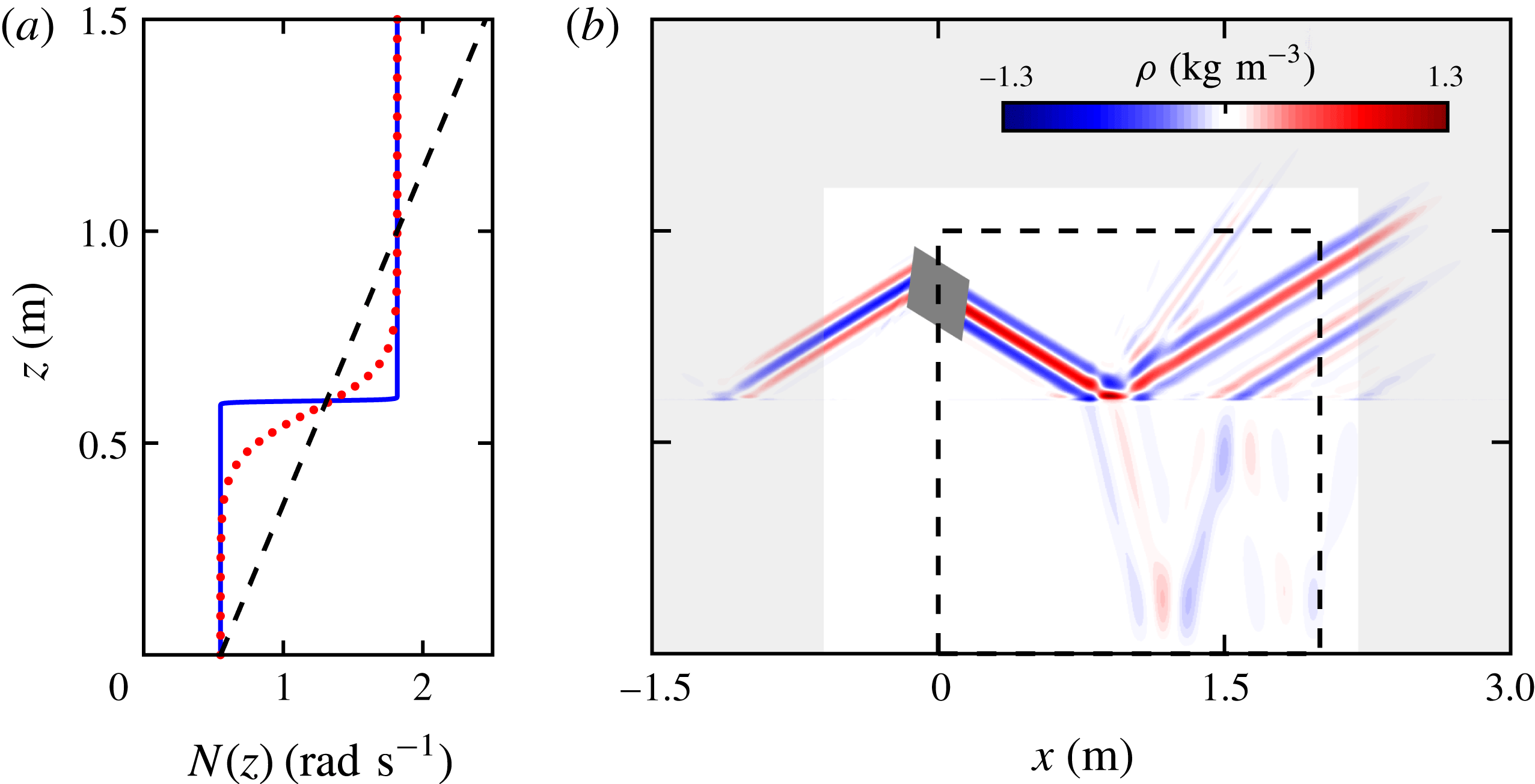
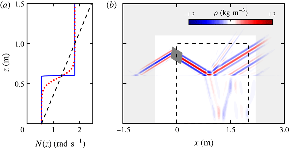
(a) The
 $N$
profile of a broad transition tanh
 $N^{2}$
(dotted red curve) and a narrow transition tanh
 $N^{2}$
profile (solid blue curve). The dashed black line is a linear
 $N$
profile. (b) The simulation domain and density perturbation field
 $\unicode[STIX]{x1D70C}$
for the narrow transition tanh
 $N^{2}$
internal wave field. Rayleigh damping is applied in the outer grey region of the field. The dark grey region indicates the location of the internal wave body forcing. The black dashed line bounds the subdomain used for analysis.
Our two-dimensional simulations span the domain
 $x\in [-1.5,3]$
m and
 $z\in [0,1.5]$
m. The simulation solves for the total density
 $\unicode[STIX]{x1D70C}_{T}$
, pressure
 $p_{T}$
and velocity
 $\boldsymbol{u}_{T}$
:
 $$\begin{eqnarray}\displaystyle \frac{\unicode[STIX]{x2202}\boldsymbol{u}_{T}}{\unicode[STIX]{x2202}t}+\boldsymbol{u}_{T}\boldsymbol{\cdot }\unicode[STIX]{x1D735}\boldsymbol{u}_{T}=-\frac{1}{\unicode[STIX]{x1D70C}_{00}}\unicode[STIX]{x1D735}p_{T}+\unicode[STIX]{x1D708}_{w}\unicode[STIX]{x1D6FB}^{2}\boldsymbol{u}_{T}-\frac{g\unicode[STIX]{x1D70C}_{T}}{\unicode[STIX]{x1D70C}_{00}}\hat{\boldsymbol{z}}, & & \displaystyle\end{eqnarray}$$
 $$\begin{eqnarray}\frac{\unicode[STIX]{x2202}\unicode[STIX]{x1D70C}_{T}}{\unicode[STIX]{x2202}t}+\boldsymbol{u}_{T}\boldsymbol{\cdot }\unicode[STIX]{x1D735}\unicode[STIX]{x1D70C}_{T}=\unicode[STIX]{x1D705}_{s}\unicode[STIX]{x1D6FB}^{2}\unicode[STIX]{x1D70C}_{T},\quad \unicode[STIX]{x1D735}\boldsymbol{\cdot }\boldsymbol{u}_{T}=0,\end{eqnarray}$$
where
 $\unicode[STIX]{x1D70C}_{00}=1000~\text{kg}~\text{m}^{-3}$
(density of water),
 $\unicode[STIX]{x1D708}_{w}=10^{-6}~\text{m}^{2}~\text{s}^{-1}$
(kinematic viscosity of water at
 $20\,^{\circ }\text{C}$
) and
 $\unicode[STIX]{x1D705}_{s}=2\times 10^{-9}~\text{m}^{2}~\text{s}^{-1}$
(the diffusivity of NaCl in water). The system is initially at rest and the density field is unperturbed. The initial density field is analytically derived from the buoyancy frequency profiles presented in figure 2(a). The boundary conditions at the bottom and top are no slip and free slip, respectively. The left and right boundaries are set to be periodic; however, Rayleigh damping is used along the perimeter of the domain (see figure 2
b), thus forcing the velocity to be negligible at the left and right boundary.
The internal wave beam is produced by using a momentum source that forms a rectangle with height 0.15 m and width 0.04 m, centred at
 $(-0.02,0.8)$
m and rotated to match the internal wave beam angle corresponding to the buoyancy frequency at
 $z=0.8$
m. The wave beam velocity imposed is
 $$\begin{eqnarray}\displaystyle \boldsymbol{u}_{T}=\unicode[STIX]{x1D714}{\mathcal{A}}(\tilde{z})\sin (\unicode[STIX]{x1D714}t-k_{\tilde{z}}\tilde{z})\hat{\tilde{\boldsymbol{x}}}, & & \displaystyle\end{eqnarray}$$
with an amplitude profile given by
 $$\begin{eqnarray}\displaystyle {\mathcal{A}}(\tilde{z})=\exp (-(\tilde{z})^{2}/0.0022), & & \displaystyle\end{eqnarray}$$
where the lengths are in metres, the rotated coordinates
 $\tilde{x}$
and
 $\tilde{z}$
correspond to the beam tangent and normal coordinates centred at
 $\boldsymbol{x}=(-0.02,0.8)$
m, respectively,
 $\unicode[STIX]{x1D714}=2\unicode[STIX]{x03C0}/13~\text{rad}~\text{s}^{-1}$
and
 $k_{\tilde{z}}=8245~\text{m}^{-1}$
. These parameters were selected to match the experimental and numerical wave beam properties used in Allshouse et al. (Reference Allshouse, Lee, Morrison and Swinney2016). The Gaussian envelope causes the amplitude of the beam to decay nearly to zero at the edge of the forcing region. A time step size
 $\unicode[STIX]{x1D6FF}t=0.0025$
s (5200 steps per period) is sufficient for temporal convergence. Spatial convergence is obtained using an unstructured mesh with resolution
 $\unicode[STIX]{x1D6FF}x\approx 0.0014$
m inside the region
 $x\in [-0.8,1.80]$
m,
 $y\in [0.5,1.1]$
m. This high resolution region contains the beam generation, the density gradient transition for the tanh
 $N^{2}$
profiles, and generation of any additional beams. The resolution outside of this region grows to
 $\unicode[STIX]{x1D6FF}x\approx 0.0025$
m near the boundaries. Changes in the velocity field are less than 1 % when spatial and temporal resolutions are doubled.
The density perturbation field for the case where we have a rapid change in buoyancy frequency (blue line in figure 2
a) is presented in figure 2(b). The internal wave beam generated at
 $(-0.02,0.8)$
m produces a beam propagating to the right; this beam is the focus of our studies. (A beam propagating to the left is damped out by the Rayleigh damping.) The beam propagating down to the right reaches the interface at
 $z=0.6$
m at which point three beams are produced: a reflected beam to the top right at the same angle to the horizontal as the incoming beam, a transmitted beam to the bottom right that has a different angle, and a reflected second harmonic beam at approximately twice the incoming angle. This particular snapshot is shown after 23.06 periods of forcing, which is sufficient for the beam in the region of interest to reach steady state.
We note that the no-flux boundary condition for the Green’s function is not satisfied at the top boundary. As demonstrated in Allshouse et al. (Reference Allshouse, Lee, Morrison and Swinney2016), the resulting errors are small and localized to the top of the domain.
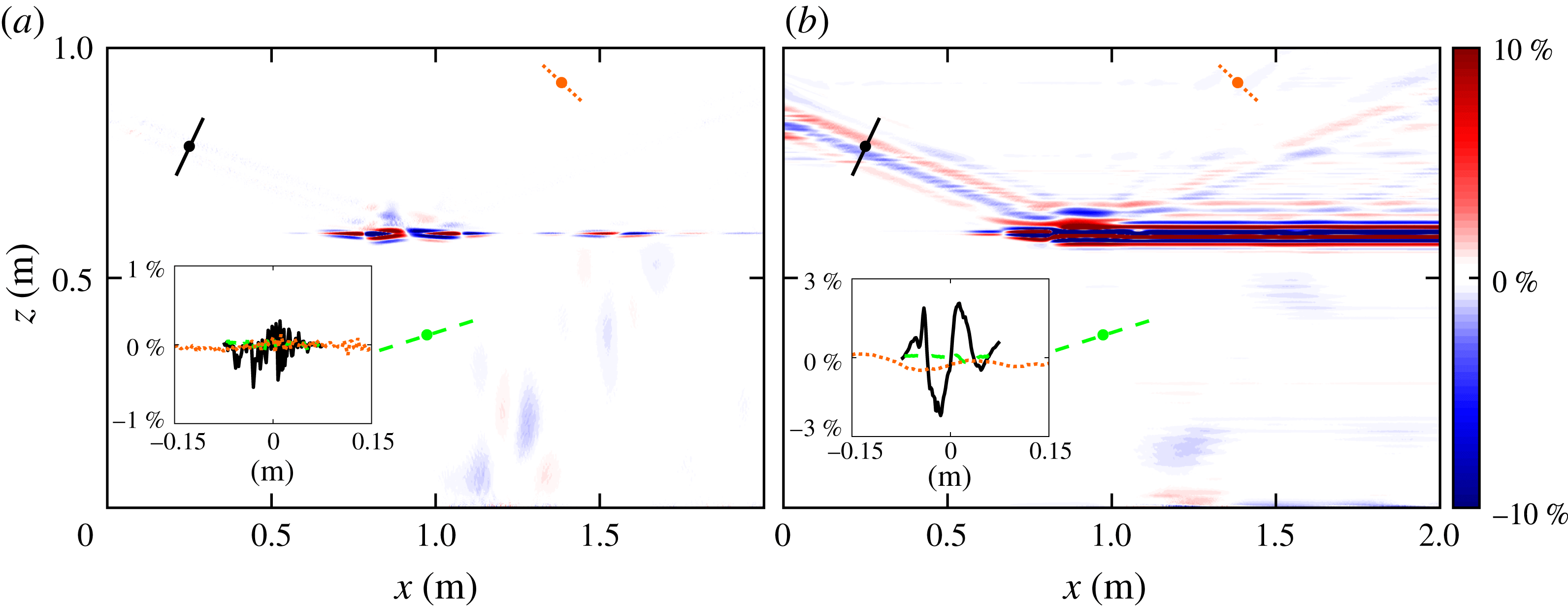
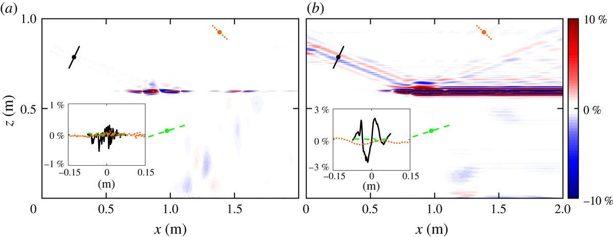
The beam-normalized per cent difference between the density-perturbation-based method and a direct numerical simulation for the velocity components (a)
 $w$
and (b)
 $u$
of an internal wave beam incident diagonally from the upper left. The insets show the per cent difference across the beam for three transects in the simulation domain: the incoming beam (solid black), the transmitted beam (dashed green) and the second harmonic beam (dotted orange). In the simulation domain the locations of the transects are shown in their respective line styles.
3.2 Verification of the tanh
 $N^{2}$
profile analysis

The vertical (2.13) and horizontal (2.14) components of the velocity and the pressure perturbation calculated from the density perturbation using the Green’s function (2.22) for the tanh
 $N^{2}$
profile are verified by comparison with the direct numerical simulations described in § 3.1. For large
 $\unicode[STIX]{x1D6FC}$
, the tanh
 $N^{2}$
profile can be approximated as a two-layer
 $N$
system, as illustrated in figure 2(a), where
 $\unicode[STIX]{x1D6FC}=4$
corresponds to a transition thickness of 0.01 m for a 95 % change in
 $N^{2}$
. This transition thickness is at least an order of magnitude smaller than the beam width and domain height. Henceforth the large
 $\unicode[STIX]{x1D6FC}$
case is called the ‘narrow transition’ tanh
 $N^{2}$
profile.
The difference between the density-perturbation-based velocity perturbation and the simulated velocity perturbation for the narrow transition tanh
 $N^{2}$
profile are presented in figure 3. To evaluate the errors in the velocity and pressure fields, we calculate the per cent difference normalized by the amplitude of the generated internal wave beam. In most of the domain, this beam-normalized per cent difference is less than 3 %, except in the transition region at
 $z=0.6$
m where there is a significant amount of nonlinearity. Because
 $u$
is found by horizontally integrating
 $\unicode[STIX]{x2202}w/\unicode[STIX]{x2202}z$
(2.14), the patches of error in
 $\unicode[STIX]{x2202}w/\unicode[STIX]{x2202}z$
result in horizontal bands of error in
 $u$
. Despite this nonlinearity, the error is small in most of the domain.
The pressure perturbation field from (a) the direct numerical simulation and (b) the Green’s function calculation from the density perturbation. (c) The beam-normalized per cent difference between the pressure fields from the two methods.
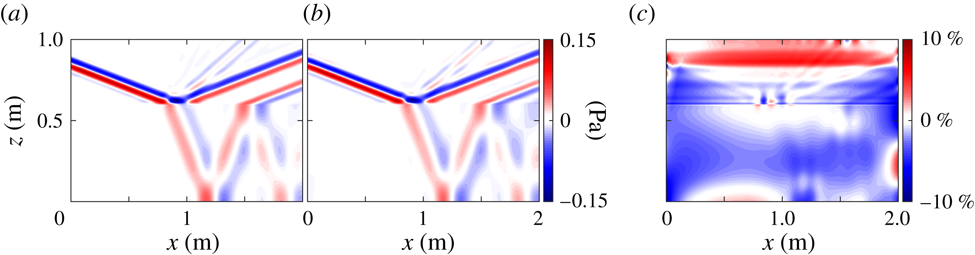
Next we investigate how well the Green’s function method calculates the pressure perturbation field from the density perturbation field. Figure 4(a) shows the simulated pressure perturbation field, and figure 4(b) shows the pressure perturbation calculated using the Green’s function method. Despite the nonlinearities in the narrow transition layer, the Green’s function method, which is based on the linear equations, yields accurate estimates of the pressure perturbation for the reflected, transmitted and second harmonic beams, as figure 4(b) illustrates. This beam-normalized per cent difference between the calculated and simulated pressure perturbation fields is presented in figure 4(c). The calculation is accurate to within 5 % over most of the domain, and to better than 10 % everywhere except within 0.02 m of where the beam enters the domain. Near the top of the domain, the Green’s function method overestimates the pressure perturbation by 4–6 %, which causes some distortion in the second harmonic, as can be seen around (1.25, 0.8) m in figure 4(a,b). The Green’s function method underestimates the pressure perturbation in the centre of the domain, but the error is less than 5 %.
The energy flux magnitude
 $|\boldsymbol{J}|$
computed in direct numerical simulations for the (a) narrow (
 $\unicode[STIX]{x1D6FC}=4$
) and (d) broad transition (
 $\unicode[STIX]{x1D6FC}=0.1$
) tanh
 $N^{2}$
profile. The beam-normalized per cent difference between the
 $x$
-component of the energy flux
 $J_{x}$
from the simulations and from the Green’s function method is shown in (b) and (e), respectively, for the narrow and broad transition regions, and corresponding results for the
 $z$
-component of the energy flux
 $J_{z}$
are in (c) and (f). For each case an inset shows the difference between the simulations and Green’s function methods is less than 5 % for most of the domain; the insets in each panel show the difference along two or three beam transects. The locations for these transects in the simulation domain are shown in their respective line styles.
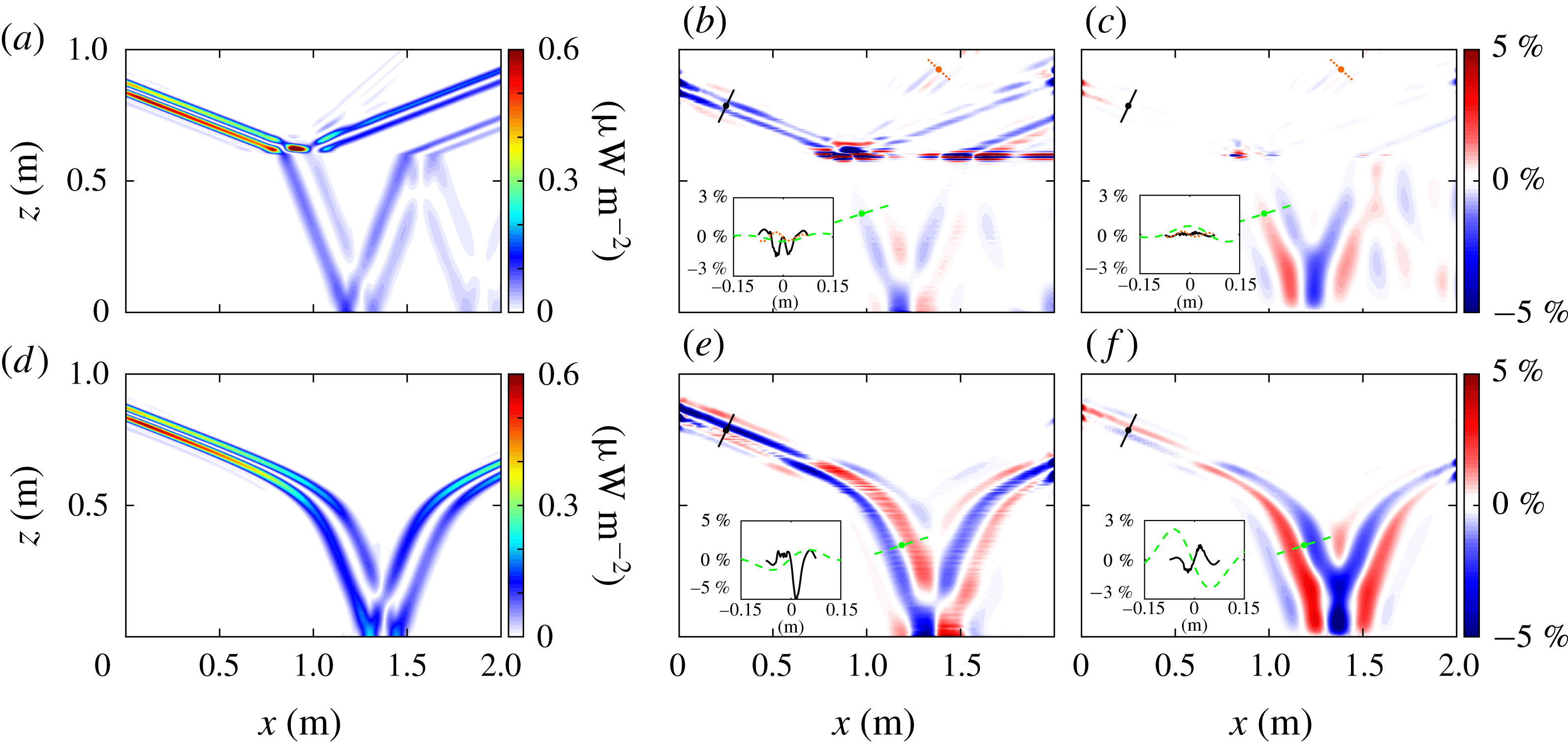
Finally, we use the calculated velocity and pressure perturbation fields to compare the energy flux
 $\boldsymbol{J}$
directly from the numerical simulations with the flux computed from the Green’s function analysis. The magnitude of the energy flux from the simulations is presented for the narrow transition tanh
 $N^{2}$
profile in figure 5(a). For the narrow transition region case, the energy flux for the reflected beam is higher than for the transmitted beam and an order of magnitude greater than in the second harmonic. The beam-normalized per cent differences of the horizontal and vertical energy flux are presented in figures 5(b) and 5(c), respectively. Outside of the immediate vicinity of the interface region at
 $z=0.6$
m, the per cent difference is less than 3 %. The accumulated error from multiplying the calculated velocity and pressure perturbation to obtain the flux components is large at the narrow transition interface as a consequence of error in the horizontal velocity perturbation, which is compensated to some extent by a more accurate pressure perturbation calculation at the interface. The error is smaller for
 $J_{z}(x,z)$
than for
 $J_{x}(x,z)$
because the vertical velocity is more accurate than the horizontal velocity. In the lower half of the domain, the magnitude of the energy flux is underestimated due to underestimation of the pressure perturbation. The insets show that the error along three beam transects is mostly smaller than 3 % for the narrow transition simulation.
We also simulate a tanh
 $N^{2}$
profile with a broader transition thickness layer of 0.31 m (
 $\unicode[STIX]{x1D6FC}=0.1$
). We omit the comparison of the velocity and pressure perturbations for brevity and instead examine the energy fluxes, as shown in figure 5. The energy flux field for the broader tanh
 $N^{2}$
profile is presented in figure 5(d). The internal wave beam passes through the broad transition without reflection because there are no rapid changes in buoyancy frequency. This smooth transition reduces the nonlinearities, so there are significantly smaller errors in the velocity perturbation field and thus the energy flux field as compared to the narrow transition tanh
 $N^{2}$
. The magnitude of the energy flux decreases as the beam widens in the bottom of the domain and then increases again as the beam narrows after reflection. Beam-normalized per cent differences are presented for the horizontal and vertical energy flux in figures 5(e) and 5(f), respectively. There is a change of overestimating the energy flux in the top of the domain to underestimating the energy flux in the bottom of the domain. This is most clearly seen at (0.7, 0.7) m where the bands of constant phase change from red to blue and vice versa. This change is due to errors in the pressure perturbation. The two insets show that within the beam the per cent difference is consistently less than 5 %.
Figure 5(a–c) demonstrates that our method can handle rapid changes in
 $N^{2}$
, while the broad
 $N^{2}$
transition thickness in figure 5(d–f) is much more representative of ocean stratifications. Figure 5(d) shows the energy flux amplitudes and reveals that the broadening of the transition layer eliminates the reflected and second harmonic beams. Further, the error in the broad transition region in figure 5(e,f) is much smaller than in the narrow transition region in figure 5(b,c). The errors of the energy flux calculation for the two tanh
 $N^{2}$
profiles are less than 5 % except in the narrow transition region (cf. insets of figure 5).
3.3 Verification of the linear profile analysis
To verify that the theory for the linear
 $N$
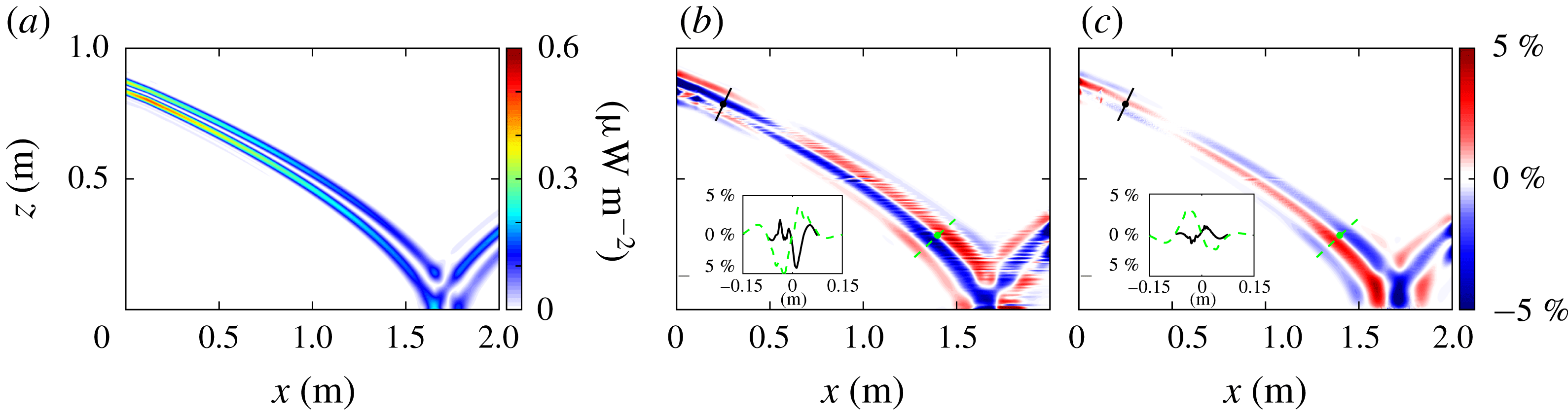
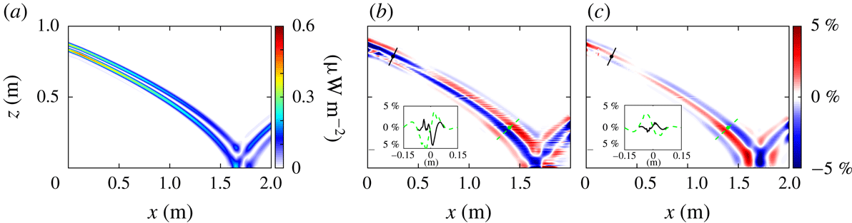
profile of § 2.3 is valid, we perform simulations analogous to those in § 3.2. The energy flux field in figure 6(a) demonstrates that the internal wave beam bends more gradually for the linear
 $N$
profile (figure 6
a) as compared to the tanh
 $N^{2}$
profiles discussed in § 3.2 (figure 5
a,d). This slower change is due to the smaller gradient of the buoyancy frequency for the linear
 $N$
profile. Again, because there are no rapid changes in
 $N$
, there are no reflection depths other than the bottom of the system, so nonlinearities are limited to the reflection point at (1.6, 0) m.
We present only the errors in the energy flux calculation; the errors in the velocity and pressure perturbation calculations are qualitatively similar to the results in figures 3 and 4. Figures 6(b) and 6(c) show the per cent difference of the horizontal and vertical components of the energy flux, respectively. As with the tanh
 $N^{2}$
profile comparisons, the errors in the energy flux field are confined to the internal wave beam. Throughout the beam the difference between the simulation and Green’s function method is less than 5 %, as illustrated by the beam transects in the insets of figure 6(b,c); the largest errors occur where the beam enters and leaves the domain and where it reflects off the bottom boundary. The transition from pressure perturbation overestimation to underestimation is highlighted by the change from red to blue and vice versa near (0.5, 0.75) m.
(a) The energy flux magnitude from the numerical simulation for the linear
 $N$
profile. The beam-normalized per cent difference between simulation and the Green’s function method for the (b)
 $J_{x}$
and (c)
 $J_{z}$
components of the energy flux; the difference is less than 5 % for most of the beam, as illustrated by insets showing the difference for two beam transects. The locations for these transects in the simulation domain are shown in their respective line styles.
4 Analysis for arbitrary
$N(z)$

Implementation of the Green’s function method is convenient for systems with stratifications where an analytic representation of the Green’s function exists. While some stratifications in the ocean and laboratory may approximately fit to these particular stratification profiles as we show in figure 1, making this density-perturbation-based calculation more general is necessary for most applications. To accomplish this generalization, we use a finite difference method to determine the pressure perturbation field. We present the method in detail along with a comparison between the Green’s function method and the finite difference method in § 4.1. Then, we apply the finite difference method to an ocean-inspired stratification in § 4.2.
4.1 Finite difference method
Since the velocity perturbation calculation does not depend on having an analytic stratification, only the calculation of the pressure perturbation field requires modification for application to general stratifications. This is accomplished by implementing a numerical solver of the second-order differential equation (2.6). The boundary conditions for this differential equation are analogous to (2.9):
 $$\begin{eqnarray}\displaystyle \left.\left(\frac{\text{d}S}{\text{d}z}-\frac{N^{2}}{2g}S\right)\right|_{z=0,\,h}=0. & & \displaystyle\end{eqnarray}$$
We solve (2.6) using a second-order finite difference method. The Robin boundary conditions are calculated to second order by adding ghost points to the top and bottom of the domain. This numerical method is applied to both the real and imaginary components for every Fourier mode. After the calculation of
 $S(z;k)$
using the finite difference method, the inverse Fourier transform of
 $S$
is then used in (2.4) to obtain the pressure perturbation field.
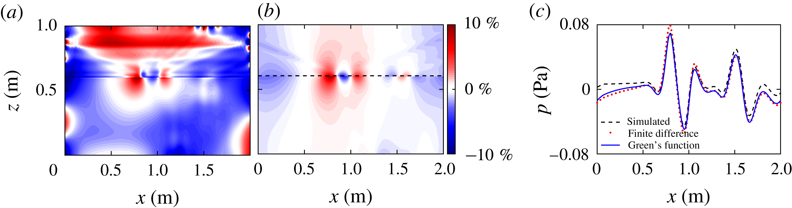
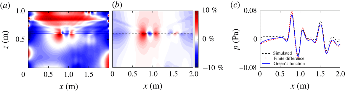
(a) The per cent difference between the finite difference (FD) and simulated pressure perturbation fields for the narrow tanh
 $N^{2}$
profile, which is essentially a two-layer system. (b) The per cent difference between the finite difference and the Green’s function based pressure perturbation fields for the narrow transition tanh
 $N^{2}$
profile. (c) Pressure perturbation profiles corresponding to the dashed black line in (b) from the narrow tanh
 $N^{2}$
simulation (black), Green’s function method (red) and finite difference method (blue) at
 $z=0.605$
m.
Applying the finite difference method to the tanh
 $N^{2}$
stratification provides a baseline for comparison to the Green’s function method. The pressure perturbation fields from the Green’s function method, the finite difference method, and the direct numerical simulations are compared in figure 7 for the narrow tanh N
 $^{2}$
stratification. Figure 7(a) presents the per cent difference between the simulated pressure field and the pressure field calculated with the finite difference method. This result is qualitatively similar to the difference between the simulated pressure field and Green’s function result presented in figure 4(c). The figure shows that the pressure perturbation fields calculated using the finite difference method differ everywhere by less than 5 % from the Green’s function pressure perturbation. The major difference between the two methods is near the narrow transition where the Green’s function method is consistently more accurate than the finite difference method; see figure 7(b). This is highlighted in figure 7(c) by comparing pressure perturbation profiles just above the transition layer. The difference is likely due to the Green’s function’s ability to accurately account for the rapid change in the buoyancy frequency when it modifies the coefficients in the calculation of the Legendre functions. The length scale of the transformed coordinate variable
 $y$
of (2.18) is set by the steepness coefficient
 $\unicode[STIX]{x1D6FC}$
. This effectively increases the spatial resolution at rapid transitions. The finite difference method can only account for variations of the scale of the original data set step size, which, in the case of the narrow transition, is too coarse.
4.2 Verification of the finite difference method
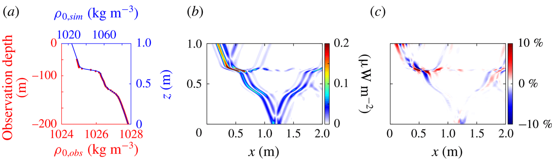
To further validate the finite difference method, we apply the method to a stratification that does not fit a simple analytic function as was the case in §§ 2 and 3. The stratification we simulate is based on a density profile measured in the ocean during the World Ocean Circulation Experiment (WOCE). The particular profile presented in figure 8(a) was measured at
 $165^{\circ }$
W,
 $51.5^{\circ }$
N on September 20th, 1994. This profile features two layers of large density gradient similar to the transitions of the tanh
 $N^{2}$
profiles. The first, more abrupt layer is centred at 30 m below the surface and the second layer is centred at 100 m. The full profile extends to a depth of 1000 m, but there is little variation in the buoyancy frequency below 200 m.
While it would be possible to apply the finite difference method to a full ocean-scale simulation, we instead simulate an equally complex stratification at the experimental scale. In order to simulate the beams in a similar domain and time scale as the analytic stratifications, we rescale the vertical coordinate and the density. We note that this is done to mimic the actual ocean profile and use it as an inspiration, rather than to model it accurately. Because the length scale of the transition layers in the simulation are small compared to the length scale of the beams, the rescaled simulation done here stress tests the method.
The first adjustment we make is to provide additional vertical space above the stratification features so that the internal wave beam is fully developed and the resulting reflection off the top of the first transition is visible. The vertical coordinate is scaled from 200 m to 0.8 m in the simulation. The density is also modified to increase the buoyancy frequency, so that the values of the buoyancy frequency are comparable to those used in the Green’s function verification. The minimum buoyancy frequency of the scaled density profile is
 $N=0.55~\text{rad}~\text{s}^{-1}$
and the maximum value is
 $N=2.40~\text{rad}~\text{s}^{-1}$
. Finally, to capture the effect of the change in
 $N$
we shift the location of forcing to be at (0.2, 1.2) m to have the internal wave beam enter from the top. The time scale and forcing periodicity match the previous simulations.
(a) Density profile from the ocean
 $\unicode[STIX]{x1D70C}_{0,obs}$
(red) and the scaled version used for simulation
 $\unicode[STIX]{x1D70C}_{0,sim}$
(blue). (b) The simulated absolute energy flux field. (c) The beam-normalized per cent difference between the simulated and finite difference energy flux fields.

The magnitude of the energy flux field is presented in figure 8(b). There are a number of reflections and transmissions due to the more complicated density profile. For the first transition layer, the internal wave beam produces reflections off the top and bottom of the transition layer at (0.5, 0.8) m and (1.0, 0.8) m, respectively. In addition to the reflected energy, some of the internal wave energy is trapped in the transition layer and is transported to the right (e.g. (1.25, 0.7) m); however, a large fraction of the energy is transmitted through the layer. Very little energy is reflected off the second layer, allowing the rest of the energy to reflect off the bottom of the domain.
The finite difference method is applied to the modified ocean density profile, and the beam-normalized per cent difference of the energy flux magnitude is presented in figure 8(c). The largest errors occur near the more abrupt transition layer. The maximum per cent difference in this region 28.1 %. There is no consistent trend with regards to under or over estimating the energy flux. Outside of the immediate region of the sharper transition, the per cent difference is generally within 5 %. Note that the method captures and accurately determines the energy flux in the reflected, transmitted and trapped internal waves outside of the highly nonlinear first reflection region.
5 Error analysis
The method for obtaining the energy flux of internal waves presented in § 2 was developed using linear theory. Therefore, as nonlinearities become significant, errors in the method become bigger. In this section we examine the effect of the nonlinearities on our method. The general properties of the errors in the velocity components and pressure perturbation shown in § 3 are discussed in § 5.1. In § 5.2 we discuss why the energy flux error comes from the error in the velocity components, which in turn arises from nonlinearities in the transition region. Then we present scaling arguments for the errors in the velocity components and the pressure perturbation due to nonlinearities. Lastly, in § 5.3 we verify our error scalings with simulations using parameter sweeps over the amplitude of the internal waves and the steepness of the density gradient region.
5.1 General qualities of the error
For both the narrow transition tanh
 $N^{2}$
profile and the ocean inspired profile, the largest errors in the calculated energy flux fields are localized in the layer where the vertical gradient in
 $N(z)$
is the largest, as can be seen in the velocity and pressure perturbation fields from the tanh
 $N^{2}$
simulation in figures 3 and 4, respectively. In particular, the vertical velocity component has large errors where the incoming beam intersects the density transition layer and partially reflects. Because the horizontal velocity is calculated as an integral of
 $\unicode[STIX]{x2202}w/\unicode[STIX]{x2202}z$
from left to right, signatures of the errors of the vertical velocity extend across most of the transition region. We show that the errors in the velocity components arise from nonlinearities due to the sharp transition in
 $N$
.
The pressure perturbation field has larger average errors than the velocity field, but there is not a clear correlation of the highest errors with the transition region. There is some error in the calculated pressure at the reflection point, but there are larger pressure errors, both in magnitude and physical extent, along the top of the domain, where the internal wave beams are generated and along the left and right boundaries, where the periodic boundary condition is imposed. The error in the pressure calculations is not strongly dependent on nonlinearities from the transition region. The spatial distribution of the error is likely due to the transformation factor in (2.5). We conclude that the errors in the energy flux (figure 5) arise primarily from the errors in the velocity field in the transition region due to nonlinearities. The scaling of the errors for both the velocity components and the pressure perturbation are obtained in § 5.2.
5.2 Scaling of errors due to nonlinearities
To determine the error scaling for the velocity components and the pressure perturbation, it is necessary to evaluate the contributions of the nonlinear terms neglected in determining (2.13) and (2.12). The full nonlinear version of the vertical velocity
 $w_{n}$
derived from (2.2) is
 $$\begin{eqnarray}\displaystyle w_{n}=\left.\left(\frac{\unicode[STIX]{x2202}\unicode[STIX]{x1D70C}}{\unicode[STIX]{x2202}t}+u\frac{\unicode[STIX]{x2202}\unicode[STIX]{x1D70C}}{\unicode[STIX]{x2202}x}\right)\right/\left(\frac{N^{2}\unicode[STIX]{x1D70C}_{0}}{g}-\frac{\unicode[STIX]{x2202}\unicode[STIX]{x1D70C}}{\unicode[STIX]{x2202}z}\right). & & \displaystyle\end{eqnarray}$$
Taking
 $\unicode[STIX]{x2202}\unicode[STIX]{x1D70C}/\unicode[STIX]{x2202}z$
to be small compared to
 $N^{2}\unicode[STIX]{x1D70C}_{0}/g=|\text{d}\unicode[STIX]{x1D70C}_{0}/\text{d}z|$
, we expand the denominator of (5.1) in
 $|\text{d}\unicode[STIX]{x1D70C}_{0}/\text{d}z|^{-1}(\unicode[STIX]{x2202}\unicode[STIX]{x1D70C}/\unicode[STIX]{x2202}z)$
to obtain
 $$\begin{eqnarray}\displaystyle w_{n}\approx \left|\frac{\text{d}\unicode[STIX]{x1D70C}_{0}}{\text{d}z}\right|^{-1}\left(\frac{\unicode[STIX]{x2202}\unicode[STIX]{x1D70C}}{\unicode[STIX]{x2202}t}+u\frac{\unicode[STIX]{x2202}\unicode[STIX]{x1D70C}}{\unicode[STIX]{x2202}x}\right)\left(1+\left|\frac{\text{d}\unicode[STIX]{x1D70C}_{0}}{\text{d}z}\right|^{-1}\frac{\unicode[STIX]{x2202}\unicode[STIX]{x1D70C}}{\unicode[STIX]{x2202}z}\right), & & \displaystyle\end{eqnarray}$$
which upon expanding to second order becomes
 $$\begin{eqnarray}\displaystyle w_{n}\approx \left|\frac{\text{d}\unicode[STIX]{x1D70C}_{0}}{\text{d}z}\right|^{-1}\left(\frac{\unicode[STIX]{x2202}\unicode[STIX]{x1D70C}}{\unicode[STIX]{x2202}t}+u\frac{\unicode[STIX]{x2202}\unicode[STIX]{x1D70C}}{\unicode[STIX]{x2202}x}+\left|\frac{\text{d}\unicode[STIX]{x1D70C}_{0}}{\text{d}z}\right|^{-1}\frac{\unicode[STIX]{x2202}\unicode[STIX]{x1D70C}}{\unicode[STIX]{x2202}t}\frac{\unicode[STIX]{x2202}\unicode[STIX]{x1D70C}}{\unicode[STIX]{x2202}z}\right), & & \displaystyle\end{eqnarray}$$
where the first term in the parentheses is first order and the second and third terms are second order. We compare the two second-order terms using dimensional scaling arguments. Assuming the propagation angle of the internal wave is not very steep or very shallow, we set the time scale of the internal wave to be
 $N^{-1}$
, using the standard internal wave dispersion relation. The density perturbation scale is
 $A\unicode[STIX]{x1D70C}_{0}$
, where
 $A$
is the dimensionless amplitude of the internal wave oscillations. The horizontal length scale is set as the beam width
 $L_{b}$
. The velocity components scale like the amplitude multiplied by the beam width divided by the time scale,
 $AL_{b}N$
. The vertical length scale in the transition region in the term
 $\unicode[STIX]{x2202}\unicode[STIX]{x1D70C}/\unicode[STIX]{x2202}z$
is set to be
 $L_{z}=N(\text{d}N/\text{d}z)^{-1}$
, which corresponds to the transition thickness, because the beam amplitude changes significantly over the transition region due to reflections. On the other hand, the vertical length scale in the term
 $\text{d}\unicode[STIX]{x1D70C}_{0}/\text{d}z$
is set to be
 $h$
, the height of the domain, since the background density changes gradually over the height of the domain. With these scalings the two second-order terms in (5.3) scale as
 $$\begin{eqnarray}\displaystyle u\frac{\unicode[STIX]{x2202}\unicode[STIX]{x1D70C}}{\unicode[STIX]{x2202}x} & {\sim} & \displaystyle AL_{b}N\frac{A\unicode[STIX]{x1D70C}_{0}}{L_{b}}=A^{2}N\unicode[STIX]{x1D70C}_{0},\end{eqnarray}$$
 $$\begin{eqnarray}\displaystyle \left|\frac{\text{d}\unicode[STIX]{x1D70C}_{0}}{\text{d}z}\right|^{-1}\frac{\unicode[STIX]{x2202}\unicode[STIX]{x1D70C}}{\unicode[STIX]{x2202}t}\frac{\unicode[STIX]{x2202}\unicode[STIX]{x1D70C}}{\unicode[STIX]{x2202}z} & {\sim} & \displaystyle \frac{h}{\unicode[STIX]{x1D70C}_{0}}A\unicode[STIX]{x1D70C}_{0}N\frac{A\unicode[STIX]{x1D70C}_{0}}{L_{z}}=A^{2}N\unicode[STIX]{x1D70C}_{0}\frac{h}{L_{z}}.\end{eqnarray}$$
Thus the ratio of sizes of the term in (5.5) to the term in (5.4) scales as
 $h/L_{z}$
, which is large for the steep transitions in
 $N$
that produce appreciable nonlinearities, because the transition thickness is then small compared to the domain height. Therefore, we drop the second-order term
 $u\,\unicode[STIX]{x2202}\unicode[STIX]{x1D70C}/\unicode[STIX]{x2202}x$
in (5.3). Then the error
 $(w_{n}-w)/w=\unicode[STIX]{x0394}w/w$
of the nonlinear vertical velocity relative to the linear vertical velocity is
 $$\begin{eqnarray}\displaystyle \text{error}=\frac{\unicode[STIX]{x0394}w}{w}\sim \frac{1}{AL_{b}N}\frac{h}{\unicode[STIX]{x1D70C}_{0}}\left(A^{2}\unicode[STIX]{x1D70C}_{0}h\frac{\text{d}N}{\text{d}z}\right)\sim \frac{Ah^{2}}{L_{b}N}\frac{\text{d}N}{\text{d}z}, & & \displaystyle\end{eqnarray}$$
where we substitute
 $L_{z}=N(\text{d}N/\text{d}z)^{-1}$
for the vertical length scale. Keeping the domain height, beam width, and the overall magnitude of
 $N$
fixed, we find that the error in the vertical velocity due to nonlinearities scales as
 $$\begin{eqnarray}\displaystyle \text{error}\sim A\frac{\text{d}N}{\text{d}z}. & & \displaystyle\end{eqnarray}$$
The full nonlinear version of the pressure equation (2.3) is given by
 $$\begin{eqnarray}\displaystyle \frac{\unicode[STIX]{x2202}^{2}p}{\unicode[STIX]{x2202}x^{2}}+\frac{\unicode[STIX]{x2202}^{2}p}{\unicode[STIX]{x2202}z^{2}}+\frac{N^{2}}{g}\frac{\unicode[STIX]{x2202}p}{\unicode[STIX]{x2202}z}=-N^{2}\unicode[STIX]{x1D70C}-g\frac{\unicode[STIX]{x2202}\unicode[STIX]{x1D70C}}{\unicode[STIX]{x2202}z}-2\unicode[STIX]{x1D70C}_{0}\left(\frac{\unicode[STIX]{x2202}u}{\unicode[STIX]{x2202}z}\frac{\unicode[STIX]{x2202}w}{\unicode[STIX]{x2202}x}-\frac{\unicode[STIX]{x2202}u}{\unicode[STIX]{x2202}x}\frac{\unicode[STIX]{x2202}w}{\unicode[STIX]{x2202}z}\right). & & \displaystyle\end{eqnarray}$$
Using the same scaling arguments as before, it can be shown that the nonlinear terms on the right-hand side of (5.8) scale approximately as
 $$\begin{eqnarray}\displaystyle -2\unicode[STIX]{x1D70C}_{0}\left(\frac{\unicode[STIX]{x2202}u}{\unicode[STIX]{x2202}z}\frac{\unicode[STIX]{x2202}w}{\unicode[STIX]{x2202}x}-\frac{\unicode[STIX]{x2202}u}{\unicode[STIX]{x2202}x}\frac{\unicode[STIX]{x2202}w}{\unicode[STIX]{x2202}z}\right)\sim A^{2}N^{2}\unicode[STIX]{x1D70C}_{0}\frac{L_{b}}{L_{z}}, & & \displaystyle\end{eqnarray}$$
while the linear terms scale as
 $$\begin{eqnarray}\displaystyle -N^{2}\unicode[STIX]{x1D70C}-g\frac{\unicode[STIX]{x2202}\unicode[STIX]{x1D70C}}{\unicode[STIX]{x2202}z}\sim AN^{2}\unicode[STIX]{x1D70C}_{0}\frac{h}{L_{z}}. & & \displaystyle\end{eqnarray}$$
The ratio of the nonlinear terms to the linear terms in (5.8) scales as
 $AL_{b}/h$
, which is small, assuming the domain height is large compared to the beam width. Thus the errors due to nonlinearities are not as significant in the pressure calculations. This was verified in simulations with the parameter sweeps; the maximum error in the pressure field does not depend strongly on
 $A\,\text{d}N/\text{d}z$
scaling. Thus we conclude that the nonlinearities primarily affect the velocity calculations.
5.3 Verification of velocity error scaling through a parameter sweep
To verify the scaling arguments, we have run a sequence of tanh
 $N^{2}$
simulations that vary the internal wave beam’s velocity amplitude and the stratification transition thickness, which changes the maximum
 $\text{d}N/\text{d}z$
. Simulations were conducted for eight velocity amplitudes ranging from
 $0.001~\text{m}~\text{s}^{-1}$
to
 $0.01~\text{m}~\text{s}^{-1}$
(the results in § 3.2 are for an amplitude of
 $0.005~\text{m}~\text{s}^{-1}$
). The two tanh
 $N^{2}$
profiles presented in § 3.2 set the upper and lower bounds on the transition layer thickness. Eight different
 $\unicode[STIX]{x1D6FC}$
values were simulated. This range corresponds to a minimum and maximum value for
 $\text{d}N/\text{d}z$
of
 $4.0~\text{m}^{-1}~\text{s}^{-1}$
and
 $112~\text{m}^{-1}~\text{s}^{-1}$
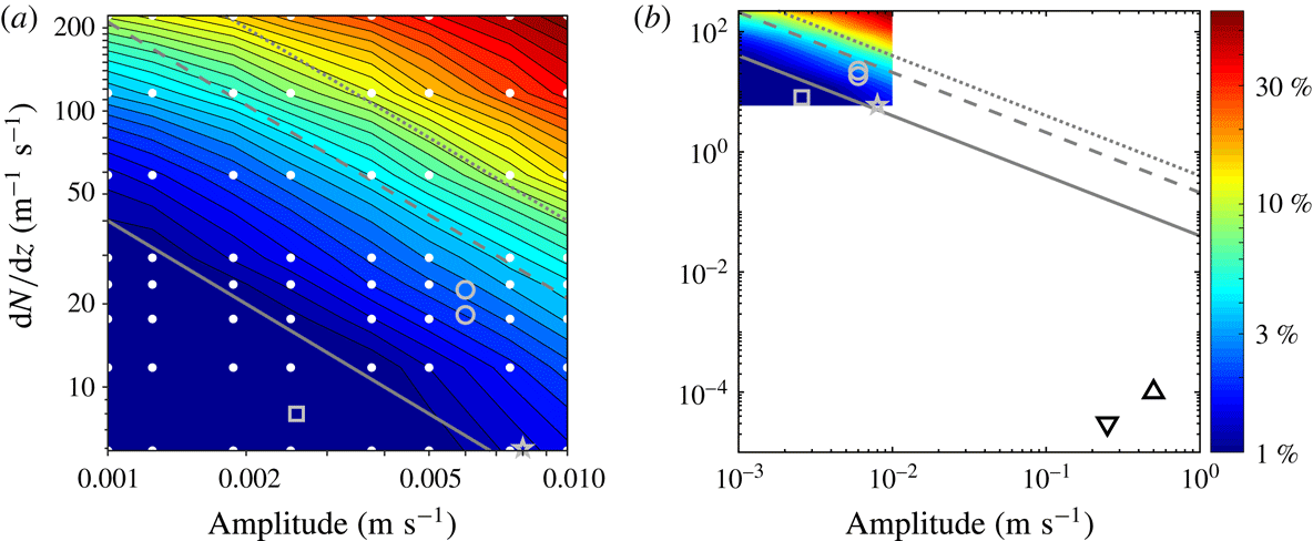
, respectively. All 64 simulations were run with the same time steps, resolution and time window as the simulations presented in § 3.2. For each simulation, we calculate the maximum absolute beam-normalized per cent difference error in the energy flux in the internal wave beam.
The simulations reveal that for most of the domain the error is less than 5 % (figure 9). The maximum error is 74 % of the beam amplitude, which occurs in the reflection region for the case with the largest vertical gradient of
 $N(z)$
(where
 $\unicode[STIX]{x1D6FC}=4$
) and the largest velocity amplitude (
 $0.01~\text{m}~\text{s}^{-1}$
). The diagonal lines with a slope of negative one indicate that the error scales approximately as
 $A\,\text{d}N/\text{d}z$
, as predicted by the scaling arguments in § 5.2.
Maximum per cent absolute difference between the energy flux from direct numerical simulations and the energy flux computed by our method as a function of the velocity amplitude and the maximum
 $\text{d}N/\text{d}z$
. The diagonal lines have slope
 $-1$
, as predicted by the scaling arguments for nonlinear terms neglected in our method, as described in § 5.2. The grey solid line corresponds to a 1 % error, the dashed grey line to a 5 % error and the dotted grey line to a 10 % error. (a) Domain of the sweep in simulation parameters, where white dots represent each simulation and symbols represent the approximate parameters for the following experiments: Mathur & Peacock (Reference Mathur and Peacock2009) (grey circles), Paoletti & Swinney (Reference Paoletti and Swinney2012) (grey star) and Ghaemsaidi et al. (Reference Ghaemsaidi, Joubaud, Dauxois, Odier and Peacock2016) (grey square). (b) A larger parameter domain that includes the internal wave beam parameters for ocean observations by Martin et al. (Reference Martin, Rudnick and Pinkel2006) (triangle) and Gerkema et al. (Reference Gerkema, Lam and Maas2004) (inverted triangle).
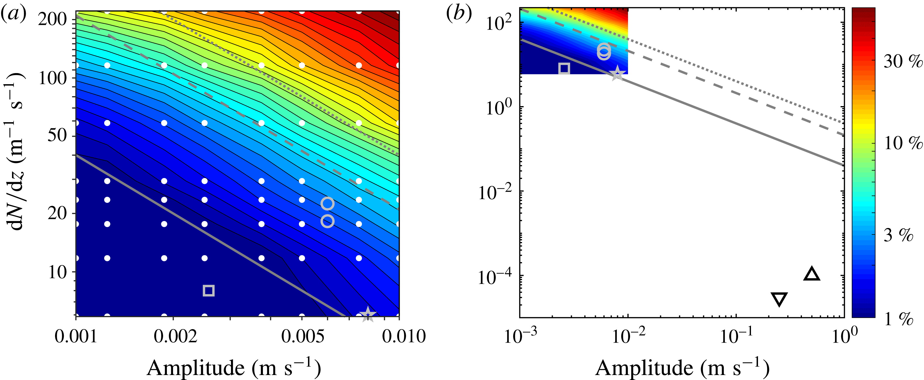
To put the computational error into context for application to experimental and potentially observational data sets, we present in figure 9(b) points that approximate the amplitude and
 $\text{d}N/\text{d}z$
values from three internal wave beam laboratory experiments that produced internal wave beams in a nonlinear stratification (Mathur & Peacock Reference Mathur and Peacock2009; Paoletti & Swinney Reference Paoletti and Swinney2012; Ghaemsaidi et al.
Reference Ghaemsaidi, Joubaud, Dauxois, Odier and Peacock2016) and two ocean observations (Gerkema et al.
Reference Gerkema, Lam and Maas2004; Martin et al.
Reference Martin, Rudnick and Pinkel2006). Although the three experiments did not have a tanh
 $N^{2}$
profile, we can still estimate the maximum value of
 $\text{d}N/\text{d}z$
, which is where we would expect the largest errors. The experiments all fall below the 5 % error line (dashed grey in figure 9(a); for the experiment of Mathur & Peacock (Reference Mathur and Peacock2009), the system falls in the regime where we would expect the method to produce errors of less than 1 %. In both observations of internal wave beams in the oceans, the amplitude is at least an order of magnitude larger than the experiments, and the
 $\text{d}N/\text{d}z$
is multiple orders of magnitude smaller (Gerkema et al.
Reference Gerkema, Lam and Maas2004; Martin et al.
Reference Martin, Rudnick and Pinkel2006).
We conclude from the parameter sweep simulations and our scaling arguments that our method yields errors due to nonlinear effects that are typically less than 1 %, and in almost all cases less than 5 %. While nonlinear effects may be the predominant source of error in analysing experimental data,
 $\text{d}N/\text{d}z$
data from ocean measurements often have large uncertainty and low spatial resolution. Also, ocean data incorporate additional complications such as background shear or tidal flow, Coriolis effects and three-dimensional internal waves. Finally, the method assumes a flat bottom to the domain, which can be accomplished by cropping out the topography, but incorporating the topography into the boundary conditions would be an avenue for future research.
6 Conclusions
We have presented two methods for calculating the instantaneous internal wave energy flux field using only data for the density perturbation field. Both methods are applicable to background density stratifications with the buoyancy frequency
 $N(z)$
varying with height
 $z$
: the first method, a Green’s function method, uses convenient analytic density stratification profiles, while the second, a finite difference method, applies to arbitrary stratification profiles.
Using our Green’s function method we obtained the instantaneous energy flux field from the density perturbation field for two profiles of
 $N(z)$
: one linear in
 $z$
and the other where
 $N(z)^{2}\propto \tanh (z)$
. The difference between the Green’s function method and our direct numerical simulations is less than 5 % outside of regions containing significant nonlinearity. Despite the Green’s function method being based on linear theory, it accurately predicts the energy flux in the transmitted and reflected beams, and even in harmonic beams, which result from significant nonlinearities.
With the finite difference method we showed how to capture the energy flux in an internal wave field containing nonlinear interactions, wave beam reflections, and second harmonic beams for any buoyancy frequency profile
 $N(z)$
. This method was compared with the Green’s function method and direct numerical simulations, and again the errors were less than 5 % for most of the domain.
An error analysis was performed to understand the scaling of errors due to nonlinearities from large gradients in
 $N$
. We argue that errors in the velocity are proportional to
 $A\,\text{d}N/\text{d}z$
(where
 $A$
is the dimensionless amplitude of the internal wave), and this scaling was verified in a series of simulations. To place the maximum per cent difference into context, parameters from experimental and observational nonlinear internal wave beam studies were used to estimate potential error from nonlinear effects. The internal wave beams fall in the parameter region where expected maximum errors are less than 5 %.
The method presented here and in Allshouse et al. (Reference Allshouse, Lee, Morrison and Swinney2016) allow detailed studies of the entire instantaneous energy flux field for an internal wave field, as contrasted with methods that yield a single global conversion rate or a time-averaged result. Our methods can be used to determine the instantaneous velocity perturbation, pressure perturbation, and energy flux fields from density perturbation data obtained in experiments using, for example, synthetic schlieren or light attenuation measurements. We emphasize that our methods require only an instantaneous density perturbation field and the background buoyancy frequency profile. The accuracy of the method relies on an accurate density perturbation field, and errors in this field will propagate through the calculated velocity and pressure fields. If the internal wave amplitude is so large as to cause experimental measurement errors, this will likely cause the nonlinear errors of the method to be large.
The Matlab GUI ‘EnergyFlux’ described in Allshouse et al. (Reference Allshouse, Lee, Morrison and Swinney2016) has been extended to include the methods discussed in this paper. The GUI requires density perturbation data, domain coordinates, time step size and the
 $N(z)$
profile. A manual and tutorial that reproduces the results in this work is available on the Matlab Central file exchange to make possible straightforward applications of the methods presented here.
Acknowledgements
We thank R. Moser for helpful discussions about the numerical simulations. The computations were done at the Texas Advanced Computing Center. M.R.A. and H.L.S. were supported by the Office of Naval Research MURI grant N000141110701, and F.M.L. and P.J.M. were supported by the US Department of Energy, Office of Science, Office of Fusion Energy Sciences, under award no. DE-FG02-04ER-54742.
Supplementary material
Supplementary material is available at https://doi.org/10.1017/jfm.2018.699.





 Open access

