1 Introduction
Various non-Newtonian materials, such as toothpaste, paint, fresh concrete, magnetite dense medium in the mineral industry and drilling fluids in the petroleum industry, exhibit a yield stress. Such materials behave like plastic solids when the imposed stress is smaller than the yield stress, and can flow like fluids when yielded. Many industrial processes involve the motion of particles in viscoplastic fluids. In the petroleum industry, a drilling fluid (normally mud) is used to transport the rock cuttings from the bottom hole to the surface (Peysson Reference Peysson2004). The yield stress is also used to control the separation of mineral particles settling in the magnetite dense medium (He, Laskowski & Klein Reference He, Laskowski and Klein2001).
Despite extensive works on the single-phase laminar flows of viscoplastic fluids (Bird, Dai & Yarusso Reference Bird, Dai and Yarusso1983; Saramito & Wachs Reference Saramito and Wachs2017), there have been limited works on the wall-bounded turbulent flows of viscoplastic fluids. Darby & Melson (Reference Darby and Melson1981) proposed a semi-empirical expression for the Fanning friction factor of the fully developed turbulent pipe flow of Bingham fluids. Anbarlooei et al. (Reference Anbarlooei, Cruz, Ramos, Santos and Freire2017) proposed a phenomenological friction equation for the turbulent pipe flow of Bingham fluids. Frigaard & Nouar (Reference Frigaard and Nouar2003) and Nouar et al. (Reference Nouar, Kabouya, Dusek and Mamou2007) examined the linear stability of Poiseuille flow of Bingham fluids. An asymmetry in the mean velocity profile of the transitional pipe flow of viscoplastic fluids was observed experimentally (Escudier et al. Reference Escudier, Poole, Presti, Dales, Nouar, Desaubry, Graham and Pullum2005; Peixinho et al. Reference Peixinho, Nouar, Desaubry and Théron2005; Esmael & Nouar Reference Esmael and Nouar2008; Güzel, Frigaard & Martinez Reference Güzel, Frigaard and Martinez2009). Esmael & Nouar (Reference Esmael and Nouar2008) attributed the reason to the existence of a robust nonlinear coherent structure characterized by two weakly modulated counter-rotating longitudinal vortices in the transitional pipe flow. The experimental results of Güzel et al. (Reference Güzel, Frigaard and Martinez2009) on the transitional pipe flow of viscoplastic fluids indicated that the plug was broken before transition commenced, and once in transition and when turbulent, the behaviour of the yield-stress fluid was somewhat similar to a (simpler) shear-thinning fluid. They also observed that the leading edges of slugs during transition were highly elongated and located off the central axis of the pipe.
Direct numerical simulations (DNS)of turbulent pipe flows of power-law fluids and Herschel–Bulkley fluids were conducted by Rudman et al. (Reference Rudman, Blackburn, Graham and Pullum2004). Singh, Rudman & Blackburn (Reference Singh, Rudman and Blackburn2017) carried out DNS of turbulent pipe flows of Bingham and Herschel–Bulkley fluids. Their results indicated that the effect of increasing yield stress was mostly similar to shear thinning in power-law fluids, and the main difference between shear thinning and yield stress was that the effect of yield stress was maximum outside the viscous sublayer whereas shear thinning had a more significant effect inside the viscous sublayer. Ohta & Miyashita (Reference Ohta and Miyashita2014) performed DNS and large eddy simulations of turbulent channel flow of various non-Newtonian fluids, with viscosity described by the power-law model and the Casson model, and their results indicated that, as for Newtonian fluids, the turbulence structures of non-Newtonian fluids could be generally normalized with locally varying viscosity. DNS of laminar and turbulent channel flow of an elastoviscoplastic fluid have been recently conducted by Rosti et al. (Reference Rosti, Izbassarov, Tammisola, Hormozi and Brandt2018), who observed that in the laminar flow regime the friction factor increased monotonically with the Bingham number, while in the turbulent regime the friction factor decreased with the Bingham number, until the flow eventually returned to a fully laminar condition for large enough yield stresses. In addition, it was shown that the near-wall streaks and the associated quasi-streamwise vortices were strongly enhanced in a highly elastoviscoplastic fluid and the flow became more correlated in the streamwise direction (Rosti et al. Reference Rosti, Izbassarov, Tammisola, Hormozi and Brandt2018).
The previous studies on the particle dynamics in viscoplastic fluids were focused on the drag on settling particles and the shape of the yield surface around the particles (Blackery & Mitsoulis Reference Blackery and Mitsoulis1997; Chhabra Reference Chhabra2006; Yu & Wachs Reference Yu and Wachs2007; Putz & Frigaard Reference Putz and Frigaard2010). Wachs & Frigaard (Reference Wachs and Frigaard2016) examined the transient dynamics of a particle settling in a Bingham fluid with an augmented Lagrangian method. Derksen (Reference Derksen2009) numerically simulated the flow of yield-stress (Bingham) liquids laden with solid particles in a mixing tank and found that more intense stirring led to a less uniform distribution of particles in the tank. No works on the interactions between particles and wall-bounded turbulent flows of viscoplastic fluids have been reported, to the best of our knowledge. The aim of the present study is to investigate the interactions between finite-size particles and turbulent channel flows of Bingham fluids using interface-resolved DNS. The essential features of the interface-resolved methods are that the interfaces between the particles and the fluid are resolved and the hydrodynamic forces on the particles are determined from the solution of the flow fields outside the particle boundaries. Such methods have been applied to simulations of particle-laden isotropic homogeneous flows (Lucci, Ferrante & Elghobashi Reference Lucci, Ferrante and Elghobashi2010; Gao, Li & Wang Reference Gao, Li and Wang2013), pipe flow (Wu, Shao & Yu Reference Wu, Shao and Yu2011; Peng & Wang Reference Peng and Wang2019), channel flows (Uhlmann Reference Uhlmann2008; Shao, Wu & Yu Reference Shao, Wu and Yu2012; Picano, Breugem & Brandt Reference Picano, Breugem and Brandt2015; Wang et al. Reference Wang, Peng, Guo and Yu2016; Yu, Vinkovic & Buffat Reference Yu, Vinkovic and Buffat2016a; Ardekani et al. Reference Ardekani, Costa, Breugem, Picano and Brandt2017; Costa et al. Reference Costa, Picano, Brandt and Breugem2018), duct flows (Lin et al. Reference Lin, Yu, Shao and Wang2017a,Reference Lin, Shao, Yu and Wangb; Fornari et al. Reference Fornari, Kazerooni, Hussong and Brandt2018) and Couette flows (Wang, Abbas & Climent Reference Wang, Abbas and Climent2017) of Newtonian fluids.
2 Numerical model
The fictitious domain (FD) method for the interface-resolved simulations of particle-laden flows was originally proposed by Glowinski et al. (Reference Glowinski, Pan, Hesla and Joseph1999). The key idea of this method is that the interior of the particles is filled with fluids and the inner fictitious fluids are enforced to satisfy the rigid-body motion constraint through a pseudo-body force, which is introduced as a distributed Lagrange multiplier in the FD formulation (Glowinski et al. Reference Glowinski, Pan, Hesla and Joseph1999). Yu & Wachs (Reference Yu and Wachs2007) developed an FD method for the particle motion in Bingham fluids. A direct-forcing fictitious domain (DF/FD) method was proposed by Yu & Shao (Reference Yu and Shao2007) and its parallel algorithm was reported by Yu et al. (Reference Yu, Lin, Shao and Wang2016b). In the present study, we develop a parallel FD method for the particle motion in Bingham fluids by combining the schemes of Yu & Wachs (Reference Yu and Wachs2007) and Yu et al. (Reference Yu, Lin, Shao and Wang2016b), and apply it to the interactions between particles and turbulent channel flows of Bingham fluids. The method is introduced briefly in the following.
2.1 Governing equations
For simplicity of description, we will consider only one particle in the following exposition. Let  $P(t)$ represent the solid domain and
 $\unicode[STIX]{x1D6FA}$ the entire domain including the interior and exterior of the solid body. The governing equations comprise the continuity equation, combined momentum equations and constitutive equations. The variational combined momentum equations were derived by Glowinski et al. (Reference Glowinski, Pan, Hesla and Joseph1999) as follows:
 $$\begin{eqnarray}\displaystyle & \displaystyle \int _{\unicode[STIX]{x1D6FA}}\unicode[STIX]{x1D70C}_{f}\frac{\text{d}\boldsymbol{u}}{\text{d}t}\boldsymbol{\cdot }\boldsymbol{v}\,\text{d}\boldsymbol{x}+\int _{\unicode[STIX]{x1D6FA}}\unicode[STIX]{x1D735}\boldsymbol{\cdot }(-p\unicode[STIX]{x1D644}+\unicode[STIX]{x1D749})\boldsymbol{\cdot }\boldsymbol{v}\,\text{d}\boldsymbol{x}-\int _{P}\unicode[STIX]{x1D740}\boldsymbol{\cdot }\boldsymbol{v}\,\text{d}\boldsymbol{x}=\mathbf{0}, & \displaystyle\end{eqnarray}$$
 $$\begin{eqnarray}\displaystyle & \displaystyle \left(1-\frac{\unicode[STIX]{x1D70C}_{f}}{\unicode[STIX]{x1D70C}_{s}}\right)\left[M\left(\frac{\text{d}\boldsymbol{U}}{\text{d}t}-\boldsymbol{g}\right)\boldsymbol{\cdot }\boldsymbol{V}+J\frac{\text{d}\unicode[STIX]{x1D74E}}{\text{d}t}\boldsymbol{\cdot }\unicode[STIX]{x1D743}\right]+\int _{P}\unicode[STIX]{x1D740}\boldsymbol{\cdot }(\boldsymbol{V}+\unicode[STIX]{x1D743}\times \boldsymbol{r})\,\text{d}\boldsymbol{x}=\mathbf{0}, & \displaystyle\end{eqnarray}$$
 $$\begin{eqnarray}\displaystyle & \displaystyle \int _{P}[\boldsymbol{u}-(\boldsymbol{U}+\unicode[STIX]{x1D74E}\times \boldsymbol{r})]\boldsymbol{\cdot }\unicode[STIX]{x1D73B}\,\text{d}\boldsymbol{x}=\mathbf{0}. & \displaystyle\end{eqnarray}$$
Here  $\unicode[STIX]{x1D70C}_{f}$,
 $\boldsymbol{u}$,
 $p$ and
 $\unicode[STIX]{x1D749}$ are the fluid density, velocity, pressure and extra stress tensor;
 $\unicode[STIX]{x1D70C}_{s}$,
 $M$,
 $J$,
 $\boldsymbol{U}$ and
 $\unicode[STIX]{x1D74E}$ are the particle density, mass, moment of inertia, translational velocity and angular velocity;
 $\unicode[STIX]{x1D644}$ is the unit tensor;
 $\unicode[STIX]{x1D740}$ is the distributed Lagrange multiplier for the constraint of rigid-body motion of the fictitious fluid in the solid domain;
 $\boldsymbol{g}$ is the gravitational acceleration;
 $\boldsymbol{r}$ is the position vector with respect to the particle centre of mass; and
 $\boldsymbol{v}$,
 $\boldsymbol{V}$,
 $\unicode[STIX]{x1D743}$ and
 $\unicode[STIX]{x1D73B}$ are the variations for the fluid velocity, the particle translational and angular velocities, and the Lagrange multiplier, respectively.
The constitutive equations for a Bingham fluid are
 $$\begin{eqnarray}\displaystyle & \displaystyle \unicode[STIX]{x1D749}=\left(2\unicode[STIX]{x1D707}+\frac{\unicode[STIX]{x1D70F}_{y}}{|\unicode[STIX]{x1D63F}|}\right)\unicode[STIX]{x1D63F}\quad \text{for}~|\unicode[STIX]{x1D749}|>\unicode[STIX]{x1D70F}_{y}, & \displaystyle\end{eqnarray}$$
 $$\begin{eqnarray}\displaystyle & \displaystyle \unicode[STIX]{x1D63F}=\mathbf{0}\quad \text{for}~|\unicode[STIX]{x1D749}|\leqslant \unicode[STIX]{x1D70F}_{y}, & \displaystyle\end{eqnarray}$$
where  $\unicode[STIX]{x1D707}$ is the fluid viscosity,
 $\unicode[STIX]{x1D70F}_{y}$ is the yield stress, and
 $\unicode[STIX]{x1D63F}$ is the rate-of-deformation tensor. The magnitude of the tensor
 $\unicode[STIX]{x1D63F}$ is defined as
 $|\unicode[STIX]{x1D63F}|=\sqrt{(1/2)\unicode[STIX]{x1D63F}\boldsymbol{ :}\unicode[STIX]{x1D63F}}$.
We employ the augmented Lagrangian method proposed by Dean & Glowinski (Reference Dean and Glowinski2002) for the solution of the constitutive equations, which are rewritten as
 $$\begin{eqnarray}\displaystyle & \displaystyle \unicode[STIX]{x1D749}=2\unicode[STIX]{x1D707}\unicode[STIX]{x1D63F}+\unicode[STIX]{x1D70F}_{y}\unicode[STIX]{x1D740}_{b}, & \displaystyle\end{eqnarray}$$
 $$\begin{eqnarray}\displaystyle & \displaystyle \unicode[STIX]{x1D740}_{b}=P_{\unicode[STIX]{x1D6EC}}(\unicode[STIX]{x1D740}_{b}+r\unicode[STIX]{x1D70F}_{y}\unicode[STIX]{x1D63F})\quad \forall ~r>0, & \displaystyle\end{eqnarray}$$
where  $P_{\unicode[STIX]{x1D6EC}}$ is a symmetry-preserving orthogonal projection operator defined by
 $$\begin{eqnarray}P_{\unicode[STIX]{x1D6EC}}(\boldsymbol{q})=\left\{\begin{array}{@{}ll@{}}\boldsymbol{q} & \text{if}~|\boldsymbol{q}|\leqslant 1,\\ \boldsymbol{q}/|\boldsymbol{q}| & \text{if}~|\boldsymbol{q}|>1.\end{array}\right.\end{eqnarray}$$
2.2 Dimensionless governing equations
The governing equations can be non-dimensionalized by introducing the following scales:  $L_{c}$ for length,
 $U_{c}$ for velocity,
 $L_{c}/U_{c}$ for time,
 $\unicode[STIX]{x1D70C}_{f}U_{c}^{2}$ for pressure and
 $\unicode[STIX]{x1D70C}_{f}U_{c}^{2}/L_{c}$ for the Lagrange multiplier. For convenience, we write the dimensionless quantities in the same form as their dimensional counterparts, unless otherwise specified. The complete set of dimensionless governing equations comprise the following three parts.
(1) Combined momentum equations:
 $$\begin{eqnarray}\displaystyle & \displaystyle \int _{\unicode[STIX]{x1D6FA}}\left(\frac{\unicode[STIX]{x2202}\boldsymbol{u}}{\unicode[STIX]{x2202}t}+\boldsymbol{u}\boldsymbol{\cdot }\unicode[STIX]{x1D735}\boldsymbol{u}\right)\boldsymbol{\cdot }\boldsymbol{v}\,\text{d}\boldsymbol{x}=\int _{\unicode[STIX]{x1D6FA}}\left[-\unicode[STIX]{x1D735}p+\frac{1}{Re}\unicode[STIX]{x1D6FB}^{2}\boldsymbol{u}+\frac{Bn}{Re}\unicode[STIX]{x1D735}\boldsymbol{\cdot }\unicode[STIX]{x1D740}_{b}\right]\boldsymbol{\cdot }\boldsymbol{v}\,\text{d}\boldsymbol{x}+\int _{P}\unicode[STIX]{x1D740}\boldsymbol{\cdot }\boldsymbol{v}\,\text{d}\boldsymbol{x}, & \displaystyle \nonumber\\ \displaystyle & & \displaystyle\end{eqnarray}$$
 $$\begin{eqnarray}\displaystyle & \displaystyle (\unicode[STIX]{x1D70C}_{r}-1)\left[V_{p}^{\ast }\left(\frac{\text{d}\boldsymbol{U}}{\text{d}t}-Fr\frac{\boldsymbol{g}}{g}\right)\boldsymbol{\cdot }\boldsymbol{V}+J^{\ast }\frac{\text{d}\unicode[STIX]{x1D74E}}{\text{d}t}\boldsymbol{\cdot }\unicode[STIX]{x1D743}\right]=-\int _{P}\unicode[STIX]{x1D740}\boldsymbol{\cdot }(\boldsymbol{V}+\unicode[STIX]{x1D743}\times \boldsymbol{r})\,\text{d}\boldsymbol{x}, & \displaystyle\end{eqnarray}$$
 $$\begin{eqnarray}\displaystyle & \displaystyle \int _{P}[\boldsymbol{u}-(\boldsymbol{U}+\unicode[STIX]{x1D74E}\times \boldsymbol{r})]\boldsymbol{\cdot }\unicode[STIX]{x1D73B}\,\text{d}\boldsymbol{x}=\mathbf{0}. & \displaystyle\end{eqnarray}$$
(2) Continuity equation:
 $$\begin{eqnarray}\int _{\unicode[STIX]{x1D6FA}}q\unicode[STIX]{x1D735}\boldsymbol{\cdot }\boldsymbol{u}\,\text{d}\boldsymbol{x}=\mathbf{0}.\end{eqnarray}$$
(3) Constitutive equations:
 $$\begin{eqnarray}\unicode[STIX]{x1D740}_{b}=P_{\unicode[STIX]{x1D6EC}}\left(\unicode[STIX]{x1D740}_{b}+r\frac{Bn}{Re}\unicode[STIX]{x1D63F}\right)\quad \forall ~r>0.\end{eqnarray}$$
In the above equations, the following dimensionless parameters are introduced:
 $$\begin{eqnarray}\displaystyle & \displaystyle \text{density ratio}\quad \unicode[STIX]{x1D70C}_{r}=\unicode[STIX]{x1D70C}_{s}/\unicode[STIX]{x1D70C}_{f}, & \displaystyle\end{eqnarray}$$
 $$\begin{eqnarray}\displaystyle & \displaystyle \text{Reynolds number}\quad Re=\frac{\unicode[STIX]{x1D70C}_{f}U_{c}L_{c}}{\unicode[STIX]{x1D707}}, & \displaystyle\end{eqnarray}$$
 $$\begin{eqnarray}\displaystyle & \displaystyle \text{Froude number}\quad Fr=\frac{gL_{c}}{U_{c}^{2}}, & \displaystyle\end{eqnarray}$$
 $$\begin{eqnarray}\displaystyle & \displaystyle \text{Bingham number}\quad Bn=\frac{\unicode[STIX]{x1D70F}_{y}L_{c}}{\unicode[STIX]{x1D707}U_{c}}. & \displaystyle\end{eqnarray}$$
The Froude number here represents the relative importance of gravity with respect to inertia. In the continuity equation (2.12),  $q$ is the pressure variation. In (2.10),
 $V_{p}^{\ast }$ and
 $J^{\ast }$ are dimensionless particle volume and moment of inertia, defined by
 $V_{p}^{\ast }=M/(\unicode[STIX]{x1D70C}_{s}L_{c}^{3})$ and
 $J^{\ast }=J/(\unicode[STIX]{x1D70C}_{s}L_{c}^{5})$. For the spherical particle,
 $V_{p}^{\ast }=(4/3)\unicode[STIX]{x03C0}(a^{\ast })^{3}$ and
 $J^{\ast }=(2V_{p}^{\ast }(a^{\ast })^{2})/5$, with
 $a^{\ast }$ being the dimensionless particle radius.
2.3 Computational scheme
2.3.1 Fractional step scheme
A fractional step (or operator-splitting) time scheme is used to decouple the system (2.9)–(2.13) into two subproblems.
(1) Fluid problem for  $\boldsymbol{u}^{\ast }$,
 $p$ and
 $\unicode[STIX]{x1D740}_{b}$:
 $$\begin{eqnarray}\displaystyle \int _{\unicode[STIX]{x1D6FA}}\frac{\boldsymbol{u}^{\ast }-\boldsymbol{u}^{n}}{\unicode[STIX]{x0394}t}\boldsymbol{\cdot }\boldsymbol{v}\,\text{d}\boldsymbol{x} & = & \displaystyle \int _{\unicode[STIX]{x1D6FA}}\left[-\unicode[STIX]{x1D735}p+\frac{1}{2Re}(\unicode[STIX]{x1D6FB}^{2}\boldsymbol{u}^{\ast }+\unicode[STIX]{x1D6FB}^{2}\boldsymbol{u}^{n})+\frac{Bn}{Re}\unicode[STIX]{x1D735}\boldsymbol{\cdot }\unicode[STIX]{x1D740}_{b}\right]\boldsymbol{\cdot }\boldsymbol{v}\,\text{d}\boldsymbol{x}\nonumber\\ \displaystyle & & \displaystyle +\,\int _{\unicode[STIX]{x1D6FA}}{\displaystyle \frac{1}{2}}(3\boldsymbol{G}^{n}-\boldsymbol{G}^{n-1})\boldsymbol{\cdot }\boldsymbol{v}\,\text{d}\boldsymbol{x}+\int _{P^{n}}\unicode[STIX]{x1D740}^{n}\boldsymbol{\cdot }\boldsymbol{v}\,\text{d}\boldsymbol{x},\end{eqnarray}$$
 $$\begin{eqnarray}\displaystyle & \displaystyle \int _{\unicode[STIX]{x1D6FA}}q\unicode[STIX]{x1D735}\boldsymbol{\cdot }\boldsymbol{u}^{\ast }\,\text{d}\boldsymbol{x}=\mathbf{0}, & \displaystyle\end{eqnarray}$$
 $$\begin{eqnarray}\displaystyle & \displaystyle \unicode[STIX]{x1D740}_{b}=P_{\unicode[STIX]{x1D6EC}}\left(\unicode[STIX]{x1D740}_{b}+r\frac{Bn}{Re}\unicode[STIX]{x1D63F}^{\ast }\right), & \displaystyle\end{eqnarray}$$
where  $G=-\boldsymbol{u}\boldsymbol{\cdot }\unicode[STIX]{x1D735}\boldsymbol{u}$.
(2) Particle problem, or rigid-body motion problem, for  $\boldsymbol{U}^{n+1}$,
 $\unicode[STIX]{x1D74E}^{n+1}$,
 $\boldsymbol{u}^{n+1}$ and
 $\unicode[STIX]{x1D740}^{n+1}$:
 $$\begin{eqnarray}\displaystyle & \!\!\displaystyle \int _{\unicode[STIX]{x1D6FA}}\left(\frac{\boldsymbol{u}^{n+1}-\boldsymbol{u}^{\ast }}{\unicode[STIX]{x0394}t}\right)\boldsymbol{\cdot }\boldsymbol{v}\,\text{d}\boldsymbol{x}=\int _{P^{n}}(\unicode[STIX]{x1D740}^{n+1}-\unicode[STIX]{x1D740}^{n})\boldsymbol{\cdot }\boldsymbol{v}\,\text{d}\boldsymbol{x}, & \displaystyle\end{eqnarray}$$
 $$\begin{eqnarray}\displaystyle & \!\!\displaystyle (\unicode[STIX]{x1D70C}_{r}-1)\left[V_{p}^{\ast \!}\left(\frac{\boldsymbol{U}^{n+1}-\boldsymbol{U}^{n}}{\unicode[STIX]{x0394}t}-Fr\frac{\boldsymbol{g}}{g}\right)\boldsymbol{\cdot }\boldsymbol{V}+J^{\ast }\frac{\unicode[STIX]{x1D74E}^{n+1}-\unicode[STIX]{x1D74E}^{n}}{\unicode[STIX]{x0394}t}\boldsymbol{\cdot }\unicode[STIX]{x1D743}\right]=-\int _{P^{n}}\unicode[STIX]{x1D740}^{n+1\!}\boldsymbol{\cdot }(\boldsymbol{V}+\unicode[STIX]{x1D743}\times \boldsymbol{r})\,\text{d}\boldsymbol{x},\hspace{-6.0pt} & \displaystyle \nonumber\\ \displaystyle & & \displaystyle\end{eqnarray}$$
 $$\begin{eqnarray}\displaystyle & \!\!\displaystyle \int _{P^{n}}[\boldsymbol{u}^{n+1}-(\boldsymbol{U}^{n+1}+\unicode[STIX]{x1D74E}^{n+1}\times \boldsymbol{r})]\boldsymbol{\cdot }\unicode[STIX]{x1D73B}\,\text{d}\boldsymbol{x}=\mathbf{0}. & \displaystyle\end{eqnarray}$$
A fractional step scheme is further used to decouple the system (2.18)–(2.20) into the following two subsystems.
(1) A Navier–Stokes problem:
 $$\begin{eqnarray}\displaystyle & \displaystyle \int _{\unicode[STIX]{x1D6FA}}\frac{\boldsymbol{u}^{\#}-\boldsymbol{u}^{n}}{\unicode[STIX]{x0394}t}\boldsymbol{\cdot }\boldsymbol{v}\,\text{d}\boldsymbol{x}=\int _{\unicode[STIX]{x1D6FA}}\left[\frac{1}{2Re}(\unicode[STIX]{x1D6FB}^{2}\boldsymbol{u}^{\#}+\unicode[STIX]{x1D6FB}^{2}\boldsymbol{u}^{n})+\frac{Bn}{Re}\unicode[STIX]{x1D735}\boldsymbol{\cdot }\unicode[STIX]{x1D740}_{b}^{n}\right]\boldsymbol{\cdot }\boldsymbol{v}\,\text{d}\boldsymbol{x} & \displaystyle\end{eqnarray}$$
 $$\begin{eqnarray}\displaystyle & \displaystyle +\int _{\unicode[STIX]{x1D6FA}}{\displaystyle \frac{1}{2}}(3\boldsymbol{G}^{n}-\boldsymbol{G}^{n-1})\boldsymbol{\cdot }\boldsymbol{v}\,\text{d}\boldsymbol{x}+\int _{P^{n}}\unicode[STIX]{x1D740}^{n}\boldsymbol{\cdot }\boldsymbol{v}\,\text{d}\boldsymbol{x}, & \displaystyle\end{eqnarray}$$
 $$\begin{eqnarray}\displaystyle & \displaystyle \int _{\unicode[STIX]{x1D6FA}}q\unicode[STIX]{x1D735}\boldsymbol{\cdot }\boldsymbol{u}^{\#}\,\text{d}\boldsymbol{x}=\mathbf{0}. & \displaystyle\end{eqnarray}$$
(2) A plasticity problem:
 $$\begin{eqnarray}\displaystyle & \displaystyle \int _{\unicode[STIX]{x1D6FA}}\frac{\boldsymbol{u}^{\ast }-\boldsymbol{u}^{\#}}{\unicode[STIX]{x0394}t}\boldsymbol{\cdot }\boldsymbol{v}\,\text{d}\boldsymbol{x}=\int _{\unicode[STIX]{x1D6FA}}\left[\frac{Bn}{Re}\unicode[STIX]{x1D735}\boldsymbol{\cdot }(\unicode[STIX]{x1D740}_{b}^{n+1}-\unicode[STIX]{x1D740}_{b}^{n})\right]\boldsymbol{\cdot }\boldsymbol{v}\,\text{d}\boldsymbol{x}, & \displaystyle\end{eqnarray}$$
 $$\begin{eqnarray}\displaystyle & \displaystyle \unicode[STIX]{x1D740}_{b}^{n+1}=P_{\unicode[STIX]{x1D6EC}}\left(\unicode[STIX]{x1D740}_{b}^{n+1}+r\frac{Bn}{Re}\unicode[STIX]{x1D63F}^{\ast }\right). & \displaystyle\end{eqnarray}$$
The plasticity system (2.27)–(2.28) is solved in the iterative way. Our scheme differs from that of Dean & Glowinski (Reference Dean and Glowinski2002) in that we retain  $\unicode[STIX]{x1D740}_{b}^{n}$ in (2.25) and (2.27), and discard the viscous diffusion term in the plasticity problem (2.27)–(2.28). Dean & Glowinski (Reference Dean and Glowinski2002) showed that the presence of the viscous diffusion term can guarantee the convergence of the iterative solution of (2.27)–(2.28) with an appropriate value of
 $r$. However, our tests indicate that there is also no convergence difficulty when the viscous diffusion term is dropped. Throughout this study, we set
 $r=Re/(2(Bn)^{2})$, as suggested by Dean & Glowinski (Reference Dean and Glowinski2002) for their scheme. The advantage of dropping the viscous diffusion term in (2.27) is that the solution of an algebraic equation set is not required when we use the finite-difference scheme to discretize the strong form of (2.27), unlike the case where this term exists.
2.3.2 Solution of Navier–Stokes problem
A finite-difference-based projection method on a half-staggered grid is used to solve the Navier–Stokes problem (2.25)–(2.26). All spatial derivatives are discretized with the second-order central difference scheme. The reader is referred to Yu et al. (Reference Yu, Lin, Shao and Wang2016b) for more details of the method. The plasticity multiplier is evaluated at the velocity nodes.
2.3.3 Solution of particle subproblem
The particle subproblem (2.21)–(2.23) was solved with the Uzawa conjugate gradient iterative method in the previous FD methods (Glowinski et al. Reference Glowinski, Pan, Hesla and Joseph1999; Yu & Wachs Reference Yu and Wachs2007). Here, we solve the particle subproblem using the DF scheme proposed by Yu & Shao (Reference Yu and Shao2007):
 $$\begin{eqnarray}\displaystyle & \displaystyle \unicode[STIX]{x1D70C}_{r}V_{p}^{\ast }\frac{\boldsymbol{U}^{n+1}}{\unicode[STIX]{x0394}t}=(\unicode[STIX]{x1D70C}_{r}-1)V_{p}^{\ast }\left(\frac{\boldsymbol{U}^{n}}{\unicode[STIX]{x0394}t}-Fr\frac{\boldsymbol{g}}{g}\right)+\int _{P}\left(\frac{\boldsymbol{u}^{\ast }}{\unicode[STIX]{x0394}t}-\unicode[STIX]{x1D740}^{n}\right)\text{d}\boldsymbol{x},\qquad & \displaystyle\end{eqnarray}$$
 $$\begin{eqnarray}\displaystyle & \displaystyle \unicode[STIX]{x1D70C}_{r}\frac{\boldsymbol{J}^{\ast }\boldsymbol{\cdot }\unicode[STIX]{x1D74E}^{n+1}}{\unicode[STIX]{x0394}t}=(\unicode[STIX]{x1D70C}_{r}-1)\left[\frac{\boldsymbol{J}^{\ast }\boldsymbol{\cdot }\unicode[STIX]{x1D74E}^{n}}{\unicode[STIX]{x0394}t}-\unicode[STIX]{x1D74E}^{n}\times (\boldsymbol{J}^{\ast }\boldsymbol{\cdot }\unicode[STIX]{x1D74E}^{n})\right]+\int _{P}\boldsymbol{r}\times \left(\frac{\boldsymbol{u}^{\ast }}{\unicode[STIX]{x0394}t}-\unicode[STIX]{x1D740}^{n}\right)\text{d}\boldsymbol{x}.\qquad & \displaystyle\end{eqnarray}$$
Note that the above equations have been reformulated so that all the terms on the right-hand side are known quantities and consequently the particle velocities  $\boldsymbol{U}^{n+1}$ and
 $\unicode[STIX]{x1D74E}^{n+1}$ are obtained without iteration. Then, the pseudo-body forces
 $\unicode[STIX]{x1D740}$ defined at the Lagrangian nodes are determined from
 $$\begin{eqnarray}\unicode[STIX]{x1D740}^{n+1}=\frac{\boldsymbol{U}^{n+1}+\unicode[STIX]{x1D74E}^{n+1}\times \boldsymbol{r}-\boldsymbol{u}^{\ast }}{\unicode[STIX]{x0394}t}+\unicode[STIX]{x1D740}^{n}.\end{eqnarray}$$
Finally, the fluid velocities  $\boldsymbol{u}^{n+1}$ at the Eulerian nodes are corrected from
 $$\begin{eqnarray}\boldsymbol{u}^{n+1}=\boldsymbol{u}^{\ast }+\unicode[STIX]{x0394}t(\unicode[STIX]{x1D740}^{n+1}-\unicode[STIX]{x1D740}^{n}).\end{eqnarray}$$
In the above manipulations, a trilinear function is used to transfer the fluid velocity from the Eulerian nodes to the Lagrangian nodes, and the pseudo-body force from the Lagrangian nodes to the Eulerian nodes.
2.4 Collision model
A particle–particle collision model is required to prevent the mutual penetration of particles. We assume that a repulsive force is activated when the gap distance between two particles is smaller than a critical value. The force has the form
 $$\begin{eqnarray}\boldsymbol{F}_{ij}=F_{0}(1-d_{ij}/d_{c})\boldsymbol{n}_{ij},\end{eqnarray}$$
where  $\boldsymbol{F}_{ij}$,
 $d_{ij}$ and
 $\boldsymbol{n}_{ij}$ are the repulsive force acting on particle
 $j$ from particle
 $i$, the gap distance and the unit normal vector pointing from the centre of particle
 $i$ to that of particle
 $j$, respectively;
 $d_{c}$ represents a cutoff distance, such that the repulsive force is activated when
 $d_{ij}<d_{c}$; and
 $F_{0}$ is the magnitude of the force at contact. We set
 $d_{c}=h$ (
 $h$ being the fluid mesh size), and
 $F_{0}=10^{3}$. The motions of the particles due to the collision force (2.33) and due to the hydrodynamic force are handled separately with the fractional step scheme. The time step for the collision model is set to be one-tenth of the latter (i.e.
 $\unicode[STIX]{x0394}t/10$) to circumvent the stiffness problem arising from the explicit integration scheme with a large value of
 $F_{0}$, as suggested by Glowinski et al. (Reference Glowinski, Pan, Hesla and Joseph1999). The collision between a particle and a wall is treated similarly, with the coefficient
 $F_{0}$ in (2.33) doubled.
2.5 Flow configuration
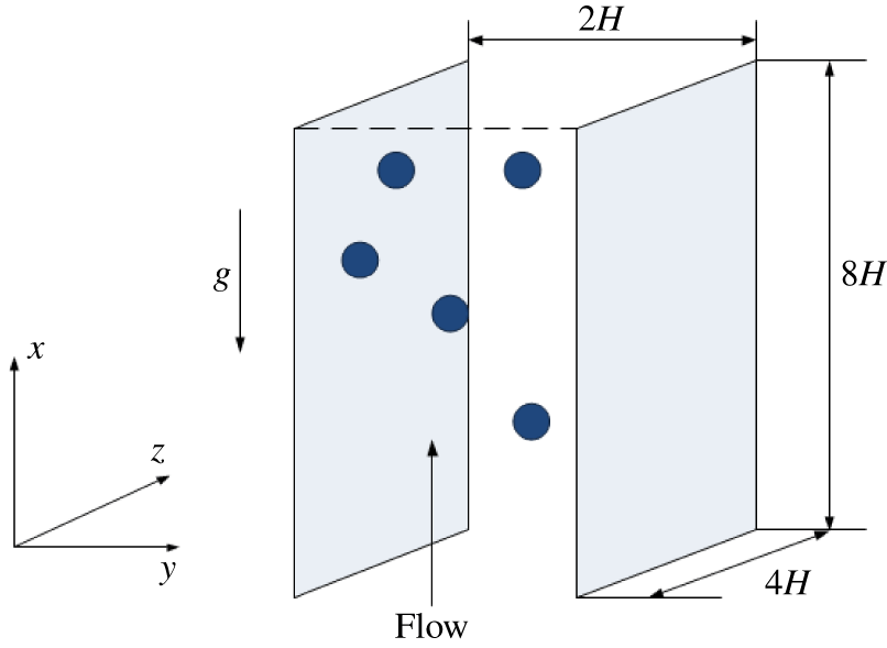
A schematic diagram of the geometrical model for the channel flow studied is shown in figure 1. We let the  $x$-axis point to the streamwise direction, the
 $y$-axis the wall-normal direction, and the
 $z$-axis the spanwise direction. The corresponding velocity components in the
 $(x,y,z)$ directions are
 $(u,v,w)$, respectively. A no-slip velocity boundary condition is imposed on the channel walls, and a periodic boundary condition is imposed in the streamwise and spanwise directions, respectively. We denote the half-width of the channel as
 $H$. In the present study, the computational domain is
 $[0,8H]\times [-H,H]\times [0,4H]$, and the numbers of grid points are
 $512\times 128\times 256$.
Geometrical model for the channel flow, with  $x$,
 $y$ and
 $z$ representing the streamwise, transverse and spanwise coordinates, respectively.

In our simulation, we take  $H$ as the characteristic length and the bulk velocity
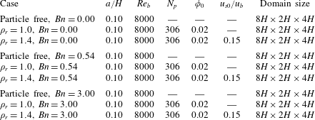
 $u_{b}$ as the characteristic velocity for the non-dimensionalization scheme. The simulation parameters are shown in table 1. The bulk Reynolds number is defined by
 $Re_{b}=\unicode[STIX]{x1D70C}_{f}2u_{b}H/\unicode[STIX]{x1D707}$, and its value is set to be 8000. The Bingham number is defined by
 $Bn=\unicode[STIX]{x1D70F}_{y}H/\unicode[STIX]{x1D707}u_{b}$. The particle radius is
 $a=0.1H$ (there are 12.8 fluid meshes per particle diameter) and the number of particles is
 $N_{p}=306$, corresponding to the particle volume fraction
 $\unicode[STIX]{x1D711}_{0}=2\,\%$. We use the ratio of the Stokes free-fall velocity of a sphere
 $u_{s0}$ to the bulk velocity
 $u_{b}$ to measure the settling effect of the particles in the vertical channel flow. The Stokes velocity
 $u_{s0}$ is defined by
 $u_{s0}=2(\unicode[STIX]{x1D70C}_{s}-\unicode[STIX]{x1D70C}_{f})ga^{2}/(9\unicode[STIX]{x1D707})$. The Froude number for the non-neutrally buoyant case can be determined from the other control parameters:
 $$\begin{eqnarray}Fr=\frac{gH}{u_{b}^{2}}=\frac{9(u_{s0}/u_{b})}{(\unicode[STIX]{x1D70C}_{r}-1)(a/H)^{2}Re_{b}}.\end{eqnarray}$$
In the present study, we only consider weak settling effects for the non-neutrally buoyant case, and  $u_{s0}/u_{b}$ is set to be 0.15. Owing to the fluid viscoplastic and inertial effects, the real particle settling velocity is much smaller than
 $0.15u_{b}$, as shown later.
Parameter settings for the simulations of particle-laden turbulent channel flows.

The accuracy of our DF/FD code for the single-phase turbulence and good mesh convergence of the turbulence statistics for the particle-laden flows (even for the coarse mesh of 6.4 points per particle diameter) have been demonstrated in Yu et al. (Reference Yu, Lin, Shao and Wang2016b). Our results on turbulent channel flow laden with finite-size neutrally buoyant particles have been compared with lattice-Boltzmann simulations using interpolated bounce-back at the fluid–solid interfaces, and the two completely different numerical approaches yielded quantitatively similar results in general (Wang et al. Reference Wang, Peng, Guo and Yu2016). Our DF/FD code has been applied to various types of particle-laden turbulent flows, including pipe flow (Wu et al. Reference Wu, Shao and Yu2011), channel flow (Shao et al. Reference Shao, Wu and Yu2012; Yu et al. Reference Yu, Lin, Shao and Wang2017) and duct flow (Lin et al. Reference Lin, Yu, Shao and Wang2017a,Reference Lin, Shao, Yu and Wangb). The accuracy of our FD method for particle sedimentation in Bingham fluids was verified in Yu & Wachs (Reference Yu and Wachs2007). The computational cost for the Bingham fluid case is one order higher than that for the Newtonian fluid case, because it typically requires more than 100 iterations for the solution of the plasticity subproblem (2.27)–(2.28). Therefore, we cannot employ a finer grid than  $512\times 128\times 256$ and thereby a smaller particle size than
 $a=0.1H$. It took around 1 million core hours for our computations.
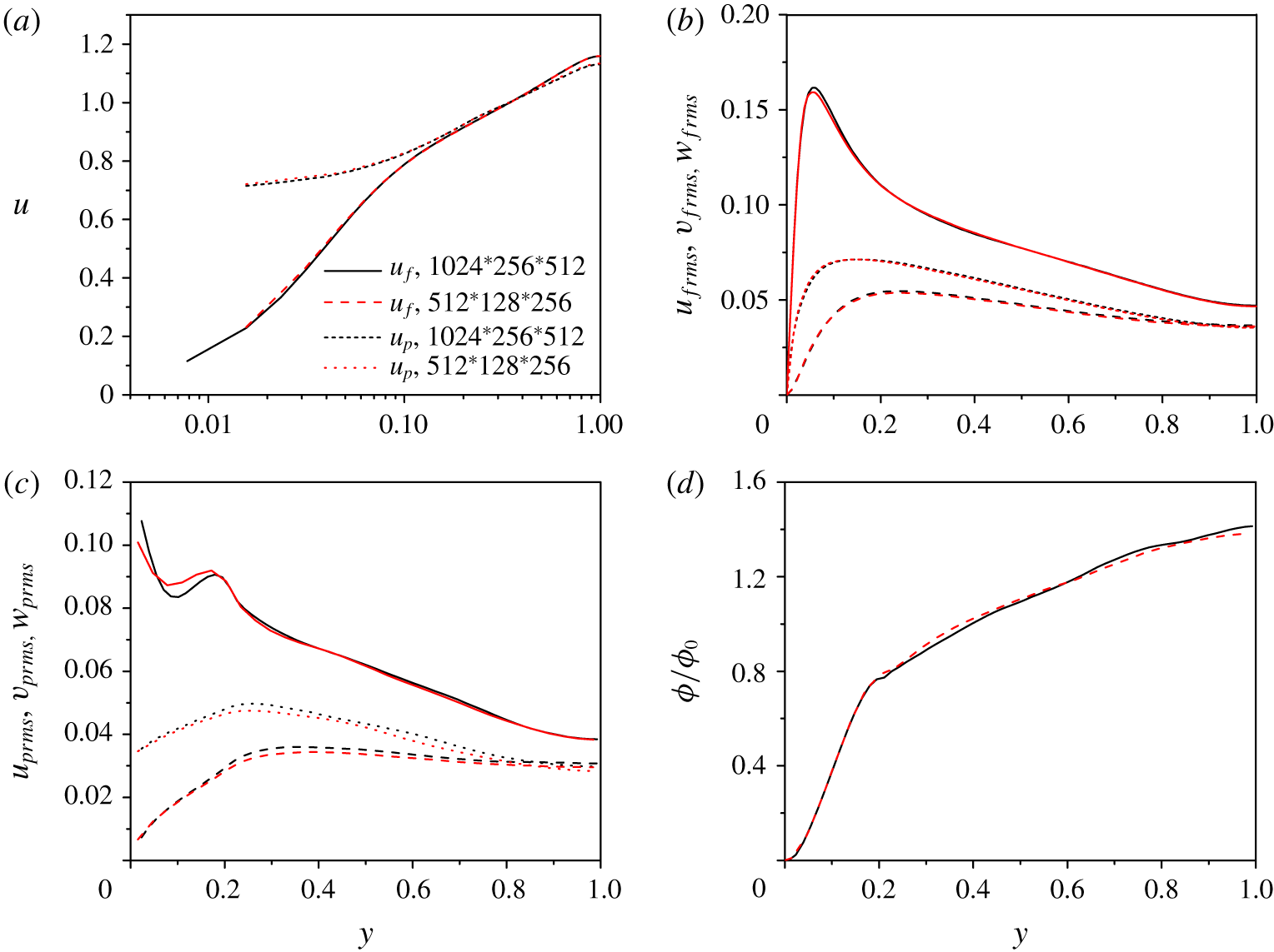
Comparison of (a) fluid and solid mean velocities, (b) fluid streamwise, spanwise and wall-normal r.m.s. velocity components, (c) solid r.m.s. velocities, and (d) particle concentration distribution obtained with two grids of  $512\times 128\times 256$ (red lines) and
 $1024\times 256\times 512$ (black lines) for
 $Re_{b}=8000$,
 $\unicode[STIX]{x1D70C}_{r}=1.4$,
 $Bn=0.00$,
 $\unicode[STIX]{x1D719}_{0}=0.02$ and
 $u_{s0}/u_{b}=0.15$.

The mesh convergence test in the work of Yu et al. (Reference Yu, Lin, Shao and Wang2016b) was performed for a large particle/fluid density ratio of around 100 (i.e. large particle inertia) and a frictional Reynolds number of 180. For the present study, the density ratio is 1 or 1.4, and the friction Reynolds number  $Re_{\unicode[STIX]{x1D70F}}$ is 243.4 for the single-phase Newtonian flow at
 $Re_{b}=8000$. The mesh size in wall units for the
 $512\times 128\times 256$ grid is around 3.8, which is relatively large. Therefore, here we conduct a mesh convergence test for the case of the Newtonian fluid and
 $\unicode[STIX]{x1D70C}_{r}=1.4$. The comparison of the fluid and solid mean velocities, the fluid and solid root-mean-square (r.m.s.) velocities and the particle concentration distribution obtained with two grids of
 $512\times 128\times 256$ and
 $1024\times 256\times 512$ is shown in figure 2. Note that for our code the grid number in each direction needs to be
 $2^{N}$ (
 $N$ is an integer). Figure 2 shows that the fluid and solid mean velocities, the fluid r.m.s. velocities and the particle concentration distribution from the two grids are in excellent agreement with each other. There are some differences between the results of the solid r.m.s. velocities, particularly the streamwise r.m.s. velocity near the wall. We think that the accuracy of the coarse mesh of
 $512\times 128\times 256$ is acceptable. The main findings of the present study are related to the single-phase flow, the effects of the particles on the fluid velocities and the particle concentration distribution. Since it is impossible for us to afford the computational cost with the fine mesh for the Bingham fluid case, the mesh of
 $512\times 128\times 256$ is chosen in the present study.
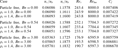
Mean fluid quantities obtained from our simulations.

3 Results and discussion
3.1 Fluid statistics
Some fluid statistics, including the bulk mean velocity  $u_{b}$, the friction velocity
 $u_{\unicode[STIX]{x1D70F}}$, the mean centreline velocity
 $u_{c}$, the friction Reynolds number
 $Re_{\unicode[STIX]{x1D70F}}$, the modified bulk Reynolds number
 $Re_{bm}$ and the friction coefficient
 $C_{f}$ are given in table 2 for the nine cases in table 1. Our computed
 $Re_{\unicode[STIX]{x1D70F}}$ (243.4) for the single-phase flow is in good agreement with the prediction from the well-established relationship
 $Re_{\unicode[STIX]{x1D70F}}\approx 0.09Re_{b}^{0.88}=244.9$ (Pope Reference Pope2000). In addition, our value 1.1578 for
 $u_{c}/u_{b}$ also agrees well with the following prediction proposed by Dean (Reference Dean1978):
 $$\begin{eqnarray}u_{c}/u_{b}=1.28Re_{b}^{-0.0116}=1.153.\end{eqnarray}$$
For a Bingham plastic, the friction Reynolds number  $Re_{\unicode[STIX]{x1D70F}}$ is defined as
 $Re_{\unicode[STIX]{x1D70F}}=\unicode[STIX]{x1D70C}_{f}u_{\unicode[STIX]{x1D70F}}H/\unicode[STIX]{x1D702}_{app}$, where
 $\unicode[STIX]{x1D702}_{app}$ is the apparent viscosity. The apparent viscosity is defined with the wall quantities,
 $\unicode[STIX]{x1D702}_{app}=\unicode[STIX]{x1D70F}_{w}/\dot{\unicode[STIX]{x1D6FE}}_{w}=\unicode[STIX]{x1D707}+\unicode[STIX]{x1D70F}_{y}\bar{\unicode[STIX]{x1D706}}_{b12w}/\dot{\unicode[STIX]{x1D6FE}}_{w}$, where
 $\bar{\unicode[STIX]{x1D706}}_{b12w}$ is the mean shear component of the plasticity tensor
 $\unicode[STIX]{x1D740}_{b}$ on the wall. The modified bulk Reynolds number
 $Re_{bm}$ in table 2 is also defined with the apparent viscosity at the wall. We found that
 $|\unicode[STIX]{x1D740}_{b}|$ in our simulations is unity or around unity everywhere in the fluid domain, which implies that the fluid is yielded almost everywhere and then roughly
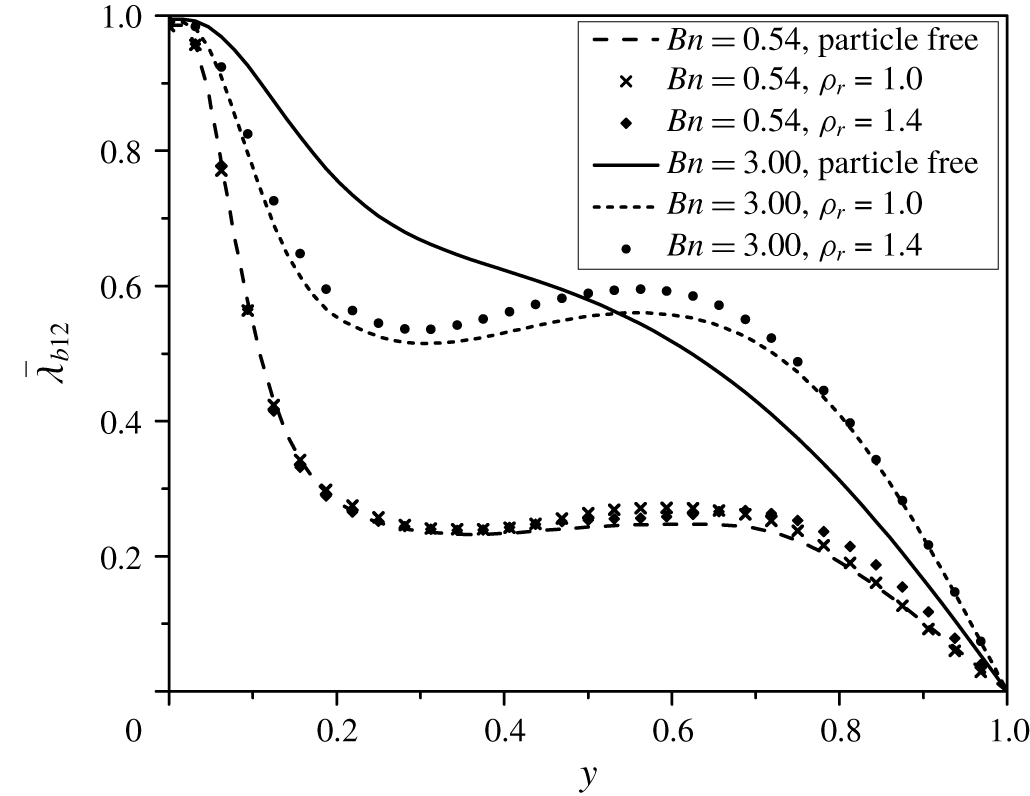
 $\bar{\unicode[STIX]{x1D706}}_{b12}=\bar{D}_{12}/|\unicode[STIX]{x1D63F}|$. Figure 3 shows the profiles of
 $\bar{\unicode[STIX]{x1D706}}_{b12}$. It can be seen that
 $\bar{\unicode[STIX]{x1D706}}_{b12}$ is almost unity at the wall and zero at the channel centre where
 $\bar{D}_{12}$ is expected to vanish due to symmetry. For
 $Bn=0.54$,
 $\bar{\unicode[STIX]{x1D706}}_{b12}$ values are close to each other for the particle-free case,
 $\unicode[STIX]{x1D70C}_{r}=1.0$ and
 $\unicode[STIX]{x1D70C}_{r}=1.4$, indicating that the distributions of the shear rate are similar for these three cases. By contrast, for
 $Bn=3.0$, the single-phase result differs significantly from those of particle-laden flows, indicating that the addition of particles modifies the flow considerably for
 $Bn=3.0$.
The mean  $\bar{\unicode[STIX]{x1D706}}_{b12}$ profiles for the turbulent channel flows of Bingham fluids.

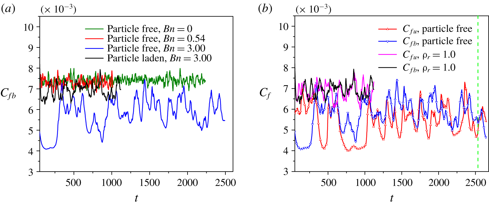
Evolution of the friction coefficients obtained from: (a) the channel bottom wall ( $y=-H$) for different cases; and (b) the top wall
 $C_{fu}$ and bottom wall
 $C_{fb}$ for
 $Bn=3.0$.

3.2 Vortex structures
An asymmetric mean velocity profile of the transitional pipe flow of viscoplastic fluids was observed experimentally (Escudier et al. Reference Escudier, Poole, Presti, Dales, Nouar, Desaubry, Graham and Pullum2005; Peixinho et al. Reference Peixinho, Nouar, Desaubry and Théron2005; Esmael & Nouar Reference Esmael and Nouar2008; Güzel et al. Reference Güzel, Frigaard and Martinez2009), as mentioned earlier in § 1. We observed similar asymmetry in the mean velocity profile of the channel flow of Bingham fluids at  $Bn=3.0$ for a long simulation time. The friction coefficient is used to reflect the flow asymmetry and intermittency here. Figure 4(b) shows the evolution of the friction coefficient obtained from the bottom wall at
 $y=-H$ and the top wall at
 $y=H$ for the particle-free and particle-laden flows at
 $Bn=3.0$ and
 $\unicode[STIX]{x1D70C}_{r}=1.0$. For convenience, we here assume that the channel is placed horizontally for the particle-free and the neurally buoyant particle-laden cases, consistent with figures 5 and 6, which show the vortex structures. For the particle-free case, the large-amplitude oscillation in figure 4(b) implies the strong temporal intermittency of the flow, and the friction coefficient for the bottom wall
 $C_{fb}$ is larger than that for the top wall
 $C_{fu}$ for most simulation times before
 $t=2000$, which implies that the flow structures in the lower half-channel are stronger than those in the upper half-channel for a long period, leading to a long-term asymmetry in the mean velocity profile. When particles are added, the temporal intermittency is reduced significantly, and the long-term domination of the friction coefficient for one wall does not occur. The statistically steady state for the particle-laden case at
 $Bn=3.0$ is reached much faster than the corresponding single-phase case, where the statistics reported below are computed with the samples for
 $t>2000$. Figure 4(a) shows the friction coefficients obtained from the bottom wall for different Bingham numbers, and one can see that the intermittency for
 $Bn=0$ and
 $Bn=0.54$ is weak compared with that for
 $Bn=3.0$.
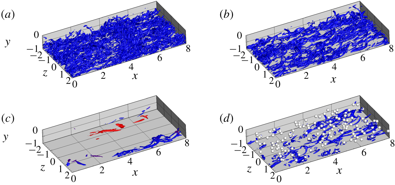
Typical vortex structures identified with the  $\unicode[STIX]{x1D706}_{ci}$ criterion of
 $\unicode[STIX]{x1D706}_{ci}=0.8$ for different cases: (a) single-phase flow at
 $Bn=0.00$,
 $y=-1$ to 0; (b) single-phase flow at
 $Bn=0.54$,
 $y=-1$ to 0; (c) single-phase flow at
 $Bn=3.0$,
 $y=-1$ to 1, at
 $t=2539$ (marked by the vertical green dashed line in figure 4b); and (d) particle-laden flow at
 $Bn=3.0$,
 $y=-1$ to 0.

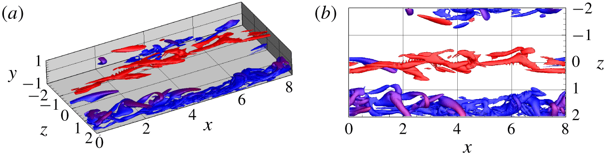
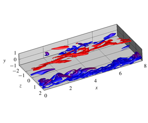
Vortex structures of the single-phase flow at  $Bn=3.0$, as for figure 5(c), but replotted with
 $\unicode[STIX]{x1D706}_{ci}=0.3$: (a) side view; and (b) top view. The colour represents the
 $y$-position, with blue for the lower half-channel and red for the upper half-channel.

The typical vortex structures for the single-phase flows at  $Bn=0$, 0.54 and 3.0 and for the particle-laden flow at
 $Bn=3.0$ are shown in figure 5. The vortex structures are identified with the isosurface of the imaginary part of the complex eigenvalue of the velocity gradient tensor, i.e. the
 $\unicode[STIX]{x1D706}_{ci}$ criterion (Zhou et al. Reference Zhou, Adrian, Balachandar and Kendall1999). Here
 $\unicode[STIX]{x1D706}_{ci}=0.8$ is chosen for the isosurfaces in figure 5. For
 $Bn=0$ and 0.54, the vortices are densely populated in the whole fluid region, exhibiting the characteristics of a fully developed turbulence state, whereas for the single-phase flow at
 $Bn=3.0$, there are not many vortices and the vortices are mainly concentrated in streamwise-extended regions or bands, surrounded by laminar flow regions, exhibiting the characteristics of a flow transitional state or strong spatial intermittency. For
 $Bn=3.0$, when particles are added, vortices can be induced by the particles and the vortices are distributed more homogeneously in space, leading to significantly reduced spatial intermittency and thereby temporal intermittency, as shown in figure 4.
The vortices of the single-phase flow at  $Bn=3.0$ in figure 5(c) are replotted with a smaller
 $\unicode[STIX]{x1D706}_{ci}$ of 0.3 in figure 6, in order to show more details of the vortex structures. It is clearer from figure 6 that the vortices are concentrated in the streamwise bands, largely segregated with the laminar flow regions in the spanwise direction. The top view (figure 6b) also shows that the vortex bands in the upper and lower half-channels are roughly staggered in the spanwise direction. Although only instantaneous vortex structures at
 $t=2539$ are plotted here, such features of the vortex distribution typically exist for other times. The possible reason for the persistently existing streamwise vortex bands is that the Bingham fluid is a strongly shear-thinning fluid, and in the vortex bands the fluid apparent viscosities are low due to high shear rates; therefore, the vortices can be more easily sustained or generated in the vortex bands. However, in the laminar flow regions, the apparent viscosities are high due to low shear rates; therefore, it is less likely for the vortices to be generated in the laminar regions. This explanation may also be applicable to the observation that the azimuthal positions of the vortices or the fast (or slow) streaks in the transitional viscoplastic pipe flow remain unchanged for a long period, which was deemed to result in the asymmetry in the mean velocity profile (Esmael & Nouar Reference Esmael and Nouar2008).
Spanwise two-point correlation functions at two  $y$-positions: (a)
 $R_{uu}$,
 $y/H=-0.875$, (b)
 $R_{vv}$,
 $y/H=-0.875$, (c)
 $R_{uu}$,
 $y/H=-0.75$, and (d)
 $R_{vv}$,
 $y/H=-0.75$.

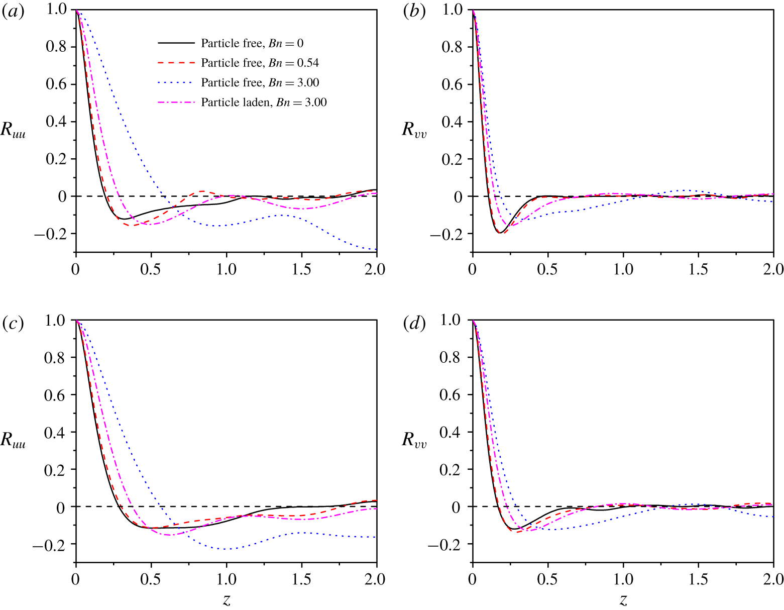
Figure 7 shows the spanwise two-point correlation functions of the velocity fluctuations at  $y/H=-0.875$ and
 $-0.75$. The correlation function is defined as
 $R_{uu}(y,\unicode[STIX]{x1D6FF}z)=\langle u^{\prime }(x,y,z,t)u^{\prime }(x,y,z+\unicode[STIX]{x1D6FF}z,t)\rangle /\langle u^{\prime \,2}(x,y,z,t)\rangle$, where the angle bracket denotes the average over time and the two homogeneous directions (i.e.
 $x$- and
 $z$-directions), and the prime represents the velocity fluctuation. As the Bingham number increases, the length corresponding to the minimum (i.e. maximum in magnitude of the negative value) of the spanwise correlation increases, which means that the spanwise spacing between the velocity streaks and the size of the streamwise large-scale vortices become larger, consistent with the vortex structures in figure 5 and the results of Rosti et al. (Reference Rosti, Izbassarov, Tammisola, Hormozi and Brandt2018). In figure 7, the negative value of
 $R_{uu}$ for the single-phase flow at
 $Bn=3.0$ does not tend to decay with distance
 $z$ and its value at
 $z=2.0$ (i.e. half of the spanwise domain size) deviates significantly away from zero, indicating that only one pair of high-speed and low-speed velocity streaks dominate in the spanwise direction during the averaging period (i.e.
 $t=2000{-}2600$), in accordance with one dominant streamwise vortex band in a half-channel in figure 5. The addition of the particles at
 $Bn=3.0$ modifies significantly the spanwise two-point correlation functions, in agreement with its considerable effects on the vortex structures in figure 5.
3.3 Effects of spanwise domain size on vortex bands
During the terminal stage of our simulations, only one dominant streamwise vortex band in each half-channel is observed (figure 5). It is of interest to examine the effect of the spanwise domain size on the spacing of the streamwise vortex bands. For this end, a new simulation with the spanwise domain size doubled (i.e.  $8H$) is started with the terminal flow fields at
 $t\approx 2600$ (figure 4) for the single-phase flow at
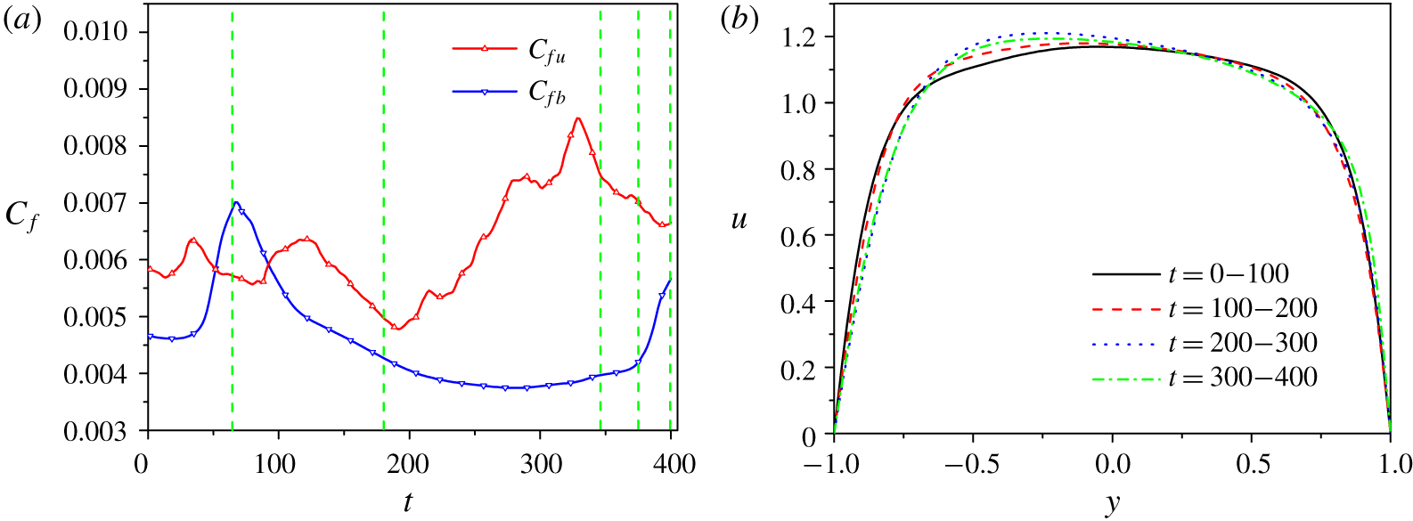
 $Bn=3.0$. Owing to the huge computational cost, the simulation is performed only for 400 dimensionless time units. The evolutions of the friction coefficients for two walls and the mean velocity profiles for every 100 dimensionless times for the single-phase turbulent channel flow at
 $Bn=3$ are shown in figure 8. For the first 100 time units, the mean frictions for two walls are comparable with each other, and accordingly the mean velocity profile is roughly symmetric. For the subsequent 300 time units, the friction on the bottom wall is smaller than that on the top wall, and the mean velocity profile becomes asymmetric, as shown in figure 8(b).
(a) Evolution of the friction coefficients obtained from the top wall  $C_{fu}$ and the bottom wall
 $C_{fb}$. (b) The mean velocity profiles for every 100 dimensionless times during the simulation times for the single-phase turbulent channel flow at
 $Bn=3.0$ with the spanwise domain size of
 $8H$.

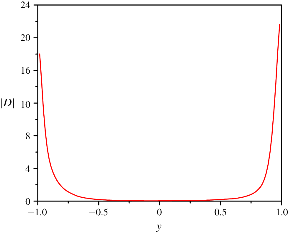
The profile for the second invariant of the strain-rate tensor for the single-phase turbulent channel flow at  $Bn=3.0$, from only spatial averaging of an instantaneous flow field at
 $t=400$, is shown in figure 9. Although from the value of
 $|\unicode[STIX]{x1D740}_{b}|$, the fluid is yielded almost everywhere, the strain rate is very close to zero in the channel centre region.
The profile for the second invariant of the strain-rate tensor for the single-phase turbulent channel flow at  $Bn=3.0$, from only spatial averaging of an instantaneous flow field at
 $t=400$.

Vortex structures identified with the  $\unicode[STIX]{x1D706}_{ci}$ criterion of
 $\unicode[STIX]{x1D706}_{ci}=0.65$ at different times (marked with the vertical green dashed lines in figure 8a): (a)
 $t=65$, (b)
 $t=180$, (c)
 $t=346$, (d)
 $t=378$, (e)
 $t=400$ (oblique view) and (f)
 $t=400$ (top view) for the single-phase turbulent channel flow at
 $Bn=3.0$ with the spanwise domain size of
 $8H$.

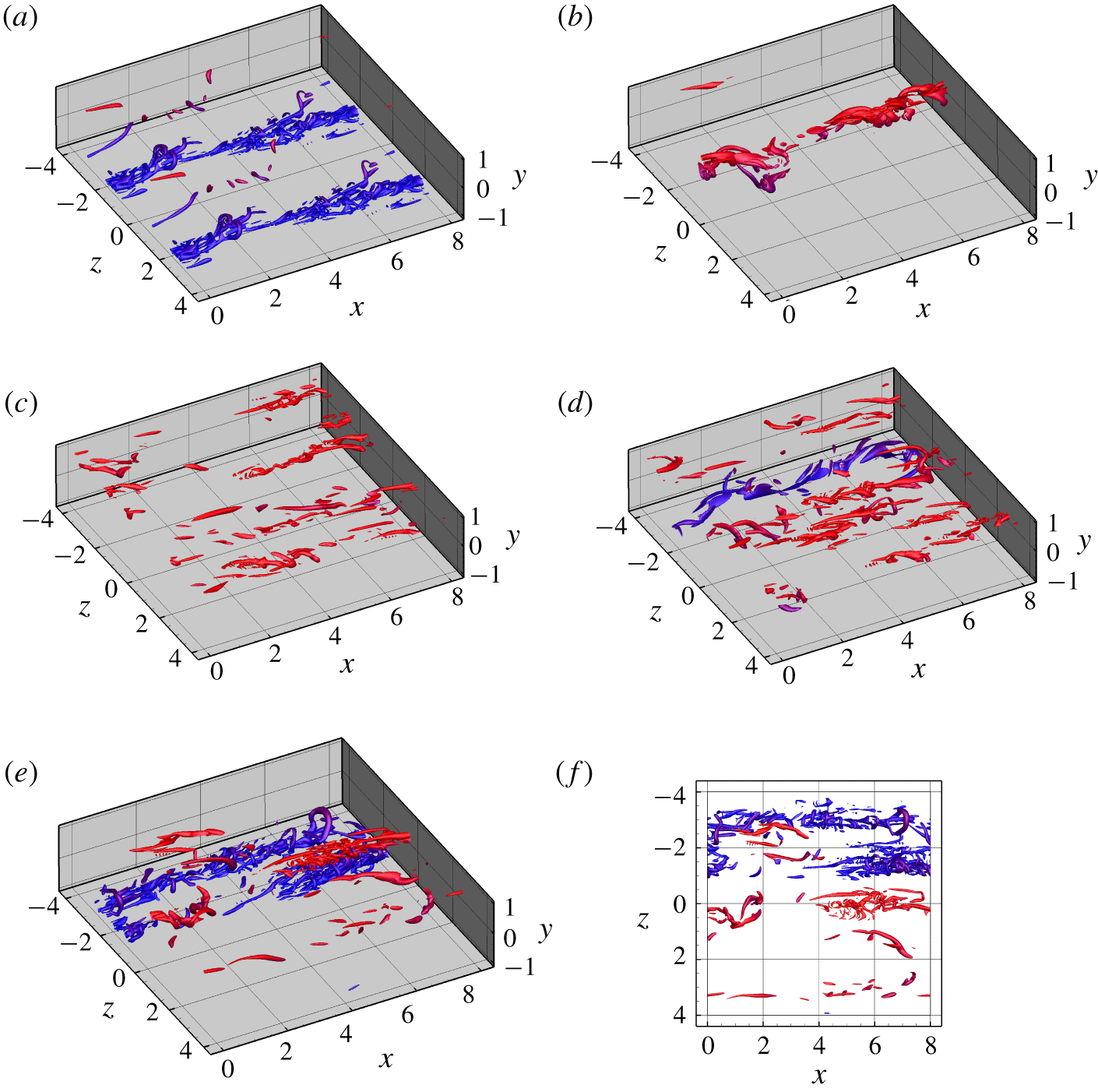
The vortex structures at  $t=65$, 180, 346, 378 and 400 (marked with the vertical green dashed lines in figure 8a) in the wider channel are plotted in figure 10. It is clear that the vortices are still preferentially concentrated in streamwise bands at any times, as in the narrower channel. However, the spanwise spacing of the bands is variable with time. At
 $t=65$, there are two main bands in the lower half-channel (figure 10a), with the same spacing as those at the initial time (i.e. the terminal time for the
 $4H$ channel simulation) (figure 5). At
 $t=180$, one vortex band in the upper half-channel appears, while the previous vortex bands in the lower half-channel have vanished (figure 10b), leading to a very low friction on the bottom wall. When there exists only one vortex band, the total wall friction is low. At
 $t=346$, there are a few vortex bands in the upper half-channel (figure 10c), leading to a large friction on the top wall. One primary vortex band forms in the lower half-channel at
 $t=378$ (figure 10d), and two bands that are close to each other occur at
 $t=400$ (figure 10e). From figure 4(b), the flow intermittency is strongest at the early stage; therefore, for the present case of the wider channel, the number of vortex bands in a half-channel may become more regular at a later stage. Accurate characterization of the vortex bands for the transitional flow needs a very large computational domain and may be a good subject for future study. In the following, we proceed to present and discuss our results for the channel with the spanwise size of
 $4H$.
3.4 Fluid mean and fluctuating velocities
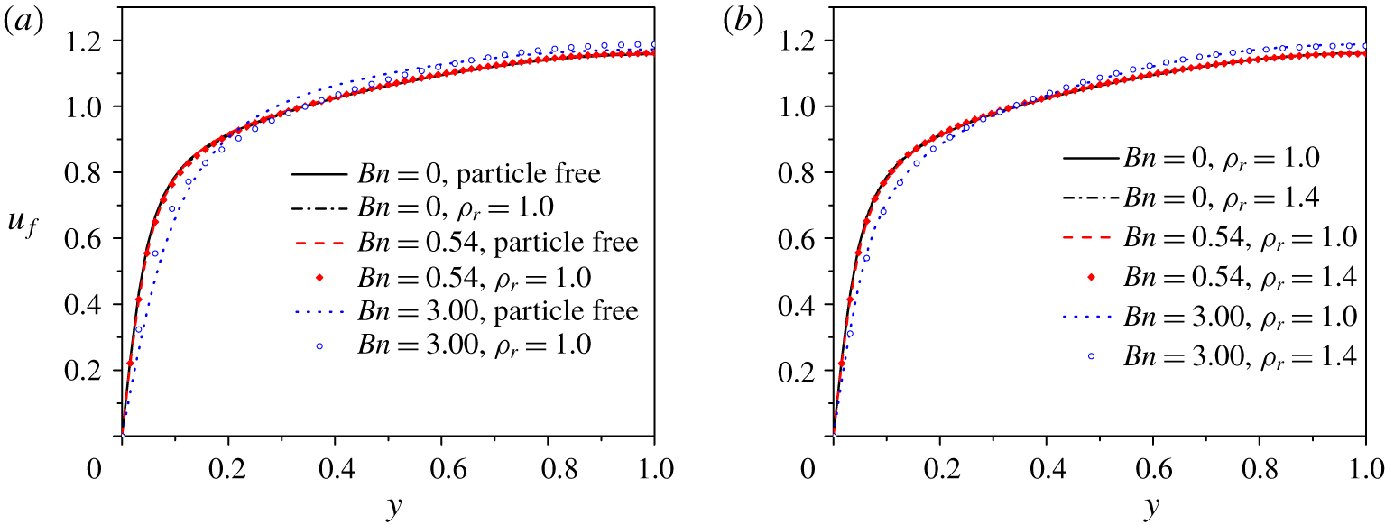
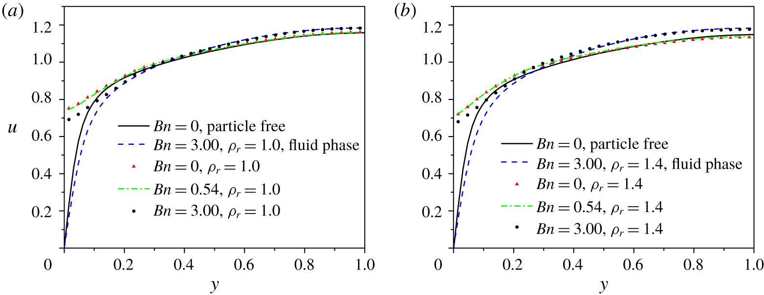
The mean velocity profiles normalized by the constant bulk velocity  $u_{b}$ are shown in figure 11. Figure 11(a) compares the particle-free cases and the neutrally buoyant particle-laden cases for
 $Bn=0.0$, 0.54 and 3.0. The near-wall velocity is smaller for a larger Bingham number, indicating that flow friction decreases with increasing Bingham number. The particle addition enhances the near-wall velocity and thereby the flow friction, particularly for
 $Bn=3.0$. Figure 11(b) compares the velocity profiles of the particle-laden flows for the neutrally buoyant (
 $\unicode[STIX]{x1D70C}_{r}=1.0$) and non-neutrally buoyant (
 $\unicode[STIX]{x1D70C}_{r}=1.4$) cases. The effects of the particle settling on the fluid mean velocity are small for the three Bingham numbers at
 $u_{s0}/u_{b}=0.15$. We will analyse the effects of the Bingham number and the particles on the flow friction via the mean two-phase momentum equation later.
Mean fluid velocity profiles  $u_{f}$ normalized by the bulk velocity
 $u_{b}$ for different cases: (a) single-phase flows and particle-laden flows (
 $\unicode[STIX]{x1D70C}_{r}=1.0$); and (b) particle-laden flows (
 $\unicode[STIX]{x1D70C}_{r}=1.0$ and
 $\unicode[STIX]{x1D70C}_{r}=1.4$).

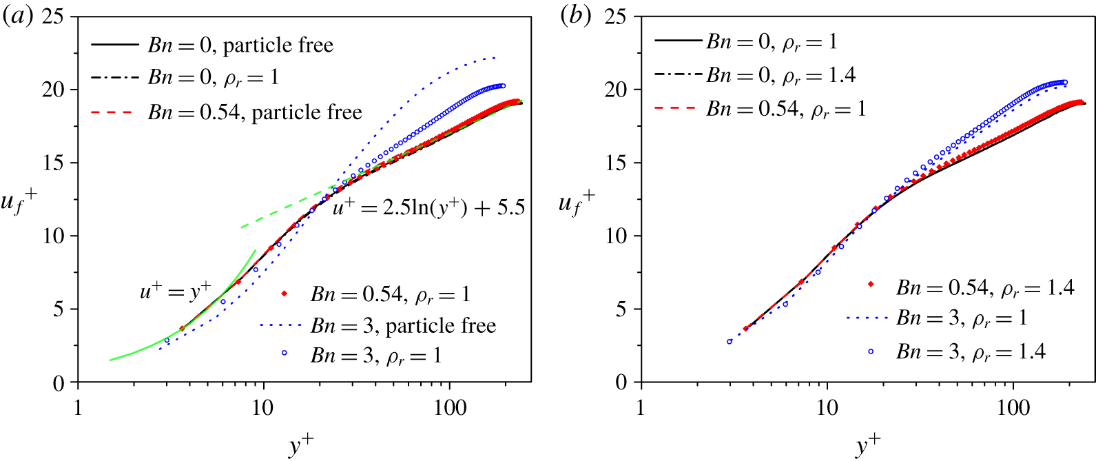
Mean fluid velocity profiles  $u_{f}^{+}$ normalized by the friction velocity
 $u_{\unicode[STIX]{x1D70F}}$ for different cases: (a) single-phase flows and particle-laden flows (
 $\unicode[STIX]{x1D70C}_{r}=1.0$); and (b) particle-laden flows (
 $\unicode[STIX]{x1D70C}_{r}=1.0$ and
 $\unicode[STIX]{x1D70C}_{r}=1.4$).

The mean velocity profiles normalized by the friction velocity  $u_{\unicode[STIX]{x1D70F}}$ are shown in figure 12. The mean velocity
 $u_{f}^{+}$ in the log region can be expressed in the form
 $$\begin{eqnarray}u_{f}^{+}=\frac{1}{\unicode[STIX]{x1D705}}\ln y^{+}+B,\end{eqnarray}$$
where  $\unicode[STIX]{x1D705}$ is the von Kármán constant and
 $B$ is another constant. Values
 $\unicode[STIX]{x1D705}=0.4$ and
 $B=5.5$ were found to be a good approximation for the single-phase flow of a Newtonian fluid (Rouson & Eaton Reference Rouson and Eaton2001; Min, Choi & Yoo Reference Min, Choi and Yoo2003; Picano et al. Reference Picano, Breugem and Brandt2015). In figure 12(a), our mean velocities in the log layer for
 $Bn=0.0$ and 0.54 can also be well fitted with
 $\unicode[STIX]{x1D705}=0.4$ and
 $B=5.5$. For
 $Bn=3.0$, the friction velocity
 $u_{\unicode[STIX]{x1D70F}}$ is much smaller than the Newtonian fluid counterpart; therefore, the maximum
 $y^{+}$ at the channel centre (i.e.
 $Re_{\unicode[STIX]{x1D70F}}$) becomes smaller and
 $u_{f}^{+}$ in the bulk region becomes larger, compared with the Newtonian fluid case. For
 $Bn=0.0$ and 0.54, the velocities in the viscous sublayer satisfy
 $u^{+}=y^{+}$ well in figure 12. This scaling does not hold for
 $Bn=3.0$, because the contribution of the yield stress to the wall friction is important for
 $Bn=3.0$.
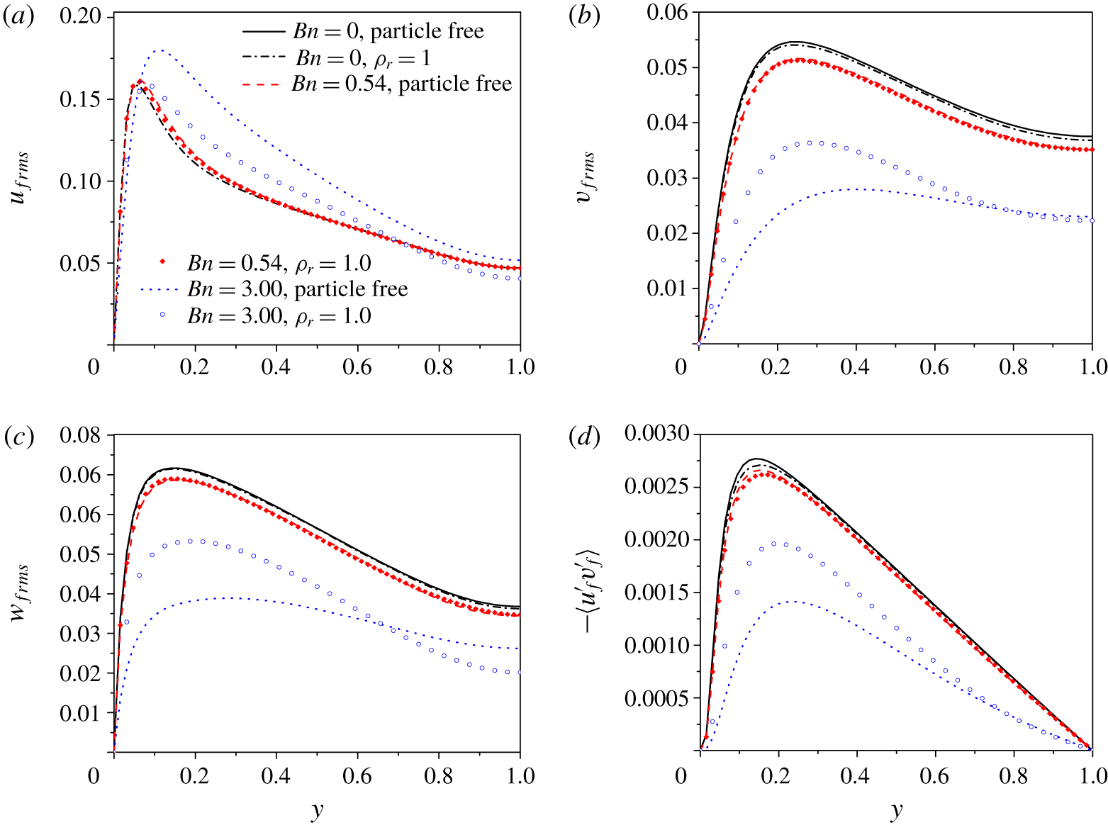
(a–c) Fluid r.m.s. velocities: (a) streamwise, (b) transverse and (c) spanwise; and (d) Reynolds shear stress for particle-free and neutrally buoyant particle-laden flows.

The r.m.s. values of the fluid velocity fluctuations in all three directions and the fluid Reynolds shear stresses for single-phase and neutrally buoyant particle-laden ( $\unicode[STIX]{x1D70C}_{r}=1.0$) flows are plotted in figure 13. For the single-phase flows, the streamwise r.m.s. velocity in the non-near-wall region increases, and the wall-normal and spanwise r.m.s. velocities and the Reynolds stress decrease, as the Bingham number increases from 0 to 3.0, consistent with the effects of the drag-reducing polymer additive on the r.m.s. velocities of the turbulent channel flow (Sureshkumar, Beris & Handler Reference Sureshkumar, Beris and Handler1997). The decrease in the wall-normal and spanwise r.m.s. velocities and the increase in the streamwise r.m.s. velocity with increasing Bingham number are associated with the decrease in the number of large-scale vortices and the increase in the size of large-scale vortices, as shown in figure 5. It was shown that the presence of particles decreases the maximum streamwise r.m.s. velocity near wall, and on the other hand increases the wall-normal and spanwise r.m.s. velocities in the vicinity of the wall, particularly at high particle volume fractions for the Newtonian fluid case (Shao et al. Reference Shao, Wu and Yu2012; Picano et al. Reference Picano, Breugem and Brandt2015; Wang et al. Reference Wang, Peng, Guo and Yu2016). Similar results of the particles on the r.m.s. velocities are observed in figure 13, clearly for
 $Bn=3.0$; the particle effects for
 $Bn=0.0$ and 0.54 are small in the present case of a low particle volume fraction and a large particle size. For
 $Bn=3.0$, the particle effects on the r.m.s. velocities can be explained by the weakening of the flow intermittency by the particles. The addition of particles slightly reduces the fluid Reynolds stress for
 $Bn=0.0$ and 0.54, while significantly enhancing the fluid Reynolds stress for
 $Bn=3.0$. The particles can significantly enhance the turbulence for
 $Bn=3.0$ by inducing vortices, where the single-phase flow is largely in the transitional state, whereas the particle effects on the fully developed turbulence at
 $Bn=0.0$ and 0.54 are complex: the particles can enhance the turbulence by inducing vortices but on the other hand can weaken the turbulence by increasing the viscous dissipation and interfering with the development of large-scale vortices.
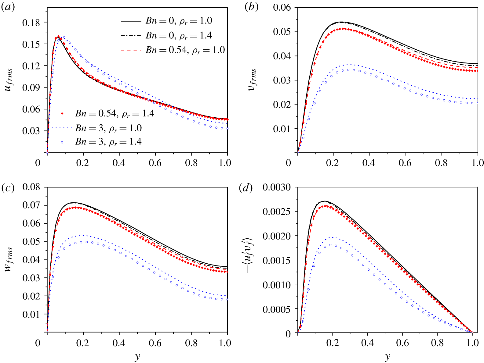
(a–c) Fluid r.m.s. velocities: (a) streamwise, (b) transverse and (c) spanwise; and (d) Reynolds shear stress for the neutrally buoyant ( $\unicode[STIX]{x1D70C}_{r}=1.0$) and non-neutrally buoyant (
 $\unicode[STIX]{x1D70C}_{r}=1.4$) particle-laden flows.

Figure 14 compares the fluid r.m.s. velocities and Reynolds stresses for  $\unicode[STIX]{x1D70C}_{r}=1.0$ and
 $\unicode[STIX]{x1D70C}_{r}=1.4$. The fluid r.m.s. velocities and Reynolds stresses are generally reduced by the particle settling effects (
 $\unicode[STIX]{x1D70C}_{r}=1.4$) for all three Bingham numbers, particularly in the bulk region. The reduction is higher for a larger Bingham number.
3.5 Solid-phase statistics
Solid-phase mean velocity profiles at different Bingham numbers for (a)  $\unicode[STIX]{x1D70C}_{r}=1.0$ and (b)
 $\unicode[STIX]{x1D70C}_{r}=1.4$. The fluid mean velocity profiles for the single-phase Newtonian flow and the particle-laden flows at
 $Bn=3.0$ are shown as references.

The profiles of the solid-phase mean velocity normalized by  $u_{b}$ for
 $\unicode[STIX]{x1D70C}_{r}=1.0$ and
 $\unicode[STIX]{x1D70C}_{r}=1.4$ are plotted in figure 15(a) and (b), respectively. The fluid mean velocity profiles for the single-phase Newtonian fluid flow and the particle-laden flows at
 $Bn=3.0$ are shown as references. The fluid mean velocities of the particle-laden flows for
 $Bn=0.0$ and 0.54 are not shown for clarity, since they are very close to that of the single-phase Newtonian fluid flow, as shown in figure 11. The solid-phase statistics are computed with the data at the grids covered by the particles. For
 $\unicode[STIX]{x1D70C}_{r}=1.0$, the fluid and the solid mean velocities are close to each other except in the near-wall region where the solid velocities are larger mainly due to the fact that most particles are in the high-speed region (Picano et al. Reference Picano, Breugem and Brandt2015; Wang et al. Reference Wang, Peng, Guo and Yu2016). For
 $\unicode[STIX]{x1D70C}_{r}=1.4$, the solid mean velocities are smaller than the fluid velocities in the channel bulk region due to particle sedimentation. The slip velocities between the two phases in the bulk region are much smaller than the particle Stokes settling velocity
 $u_{s0}=0.15u_{b}$, because of the fluid viscoplastic and inertial effects. In particular, for
 $Bn=3.0$, the slip velocity is very small. In the near-wall region, the solid mean velocities are still larger than the fluid counterparts for the case of sedimentation. We note that similar results were observed experimentally in the particle-laden flows in a vertical tube (Tsuji, Morikawa & Shiomi Reference Tsuji, Morikawa and Shiomi1984; Shokri et al. Reference Shokri, Ghaemi, Nobes and Sanders2017). The reason for the larger particle mean velocity near the wall was attributed to the facts that the particles can slip on the wall and are preferentially located in the fluid high-speed streaks (Tsuji et al. Reference Tsuji, Morikawa and Shiomi1984; Shokri et al. Reference Shokri, Ghaemi, Nobes and Sanders2017).
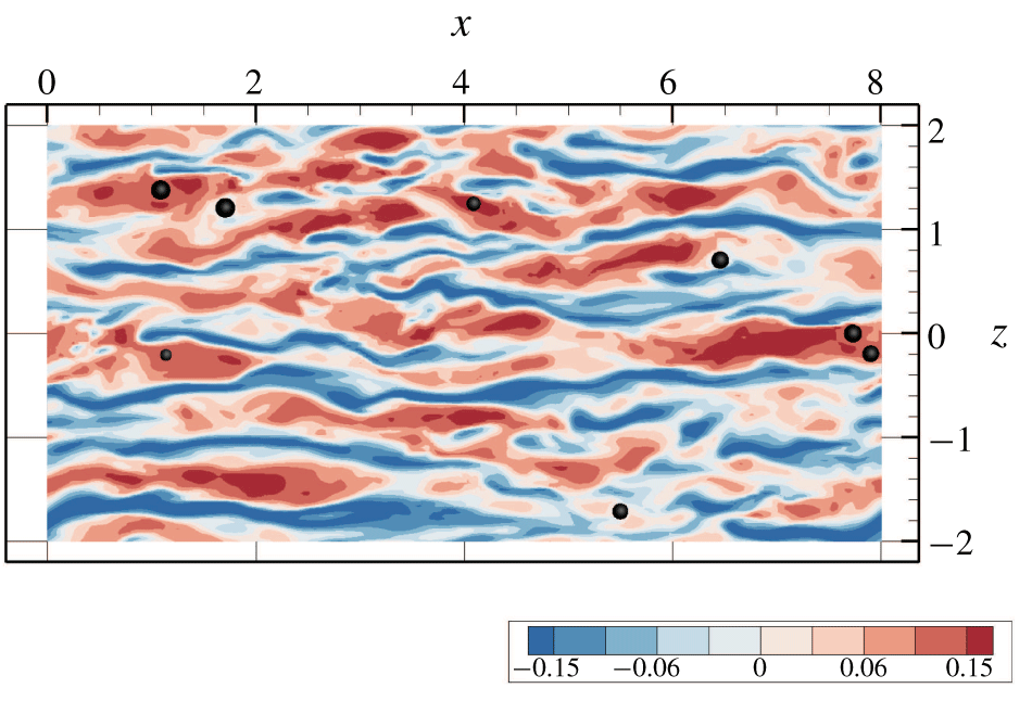
The low- and high-speed streaks and the particle cross-sections in the plane of  $y/H=-0.9$ for
 $Bn=0.0$ and
 $\unicode[STIX]{x1D70C}_{r}=1.4$ are shown in figure 16. One can see that almost all particles are located in the high-speed streaks. There are few particles in the plane near the wall due to the low volume fraction (2 %) and the particle migration towards the channel centre, as discussed later.
Particle cross-sections and low- and high-speed streaks in the plane of  $y/H=-0.9$ for
 $Bn=0.0$ and
 $\unicode[STIX]{x1D70C}_{r}=1.4$.

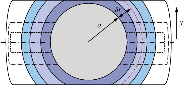
Schematic diagram of the computational model for the relative mean velocity of the fluid with respect to the particle. The averaging region is a spherical shell of thickness  $a/4$ cut by two planes located at
 $y_{0}\pm d_{y}$ (i.e. a mooncake-shaped region), where
 $y_{0}$ is the
 $y$-position of the particle centre and
 $d_{y}$ is the half height of the mooncake region.

The time for the flow field in figure 16 is randomly chosen; however, it is more rigorous to inspect the relative mean velocity of the surrounding fluid with respect to the particles. Cisse, Homann & Bec (Reference Cisse, Homann and Bec2013) and Fornari et al. (Reference Fornari, Picano, Sardina and Brandt2016b) calculated the relative mean velocity by averaging the fluid velocity in a region of a spherical shell surrounding each particle. For the turbulent channel flow with an inhomogeneous velocity distribution, it may not be appropriate to take an entire spherical shell as the averaging region. Since the particle velocity is the velocity of the particle centre, it is better to compare the particle velocity with the velocity of the fluids in the region with the  $y$-position close to that of the particle centre. Figure 17 shows the schematic diagram of our computational model for the relative mean velocity. The averaging region has a mooncake shape, i.e. a spherical shell of thickness
 $a/4$ cut by two planes located at
 $y_{0}\pm d_{y}$, where
 $y_{0}$ is the
 $y$-position of the particle centre and
 $d_{y}$ is the half height of the mooncake region.
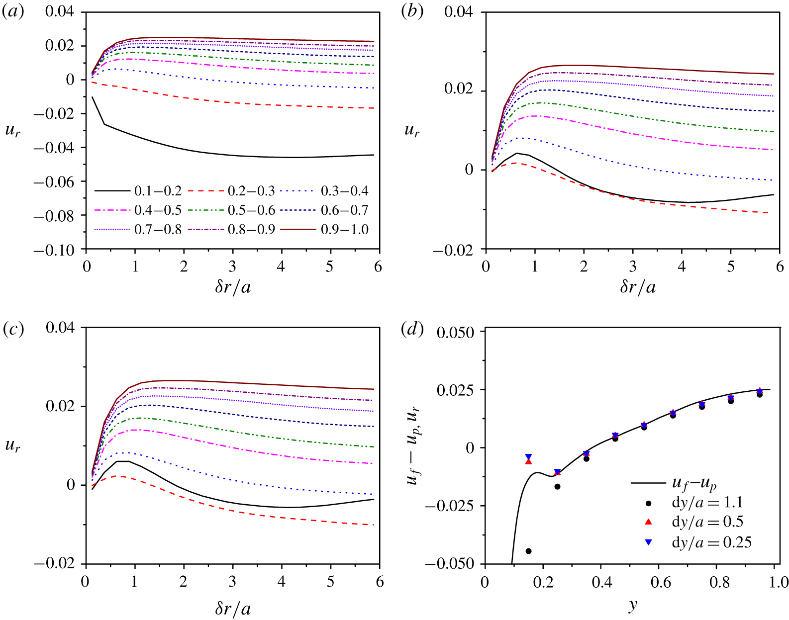
(a–c) Relative mean velocities of the fluid with respect to the particle as a function of the distance between the shell centre and the particle surface for 10 bands of width  $0.1H$ where the particle centres are located and for three averaging heights: (a)
 $d_{y}=1.1a$, (b)
 $d_{y}=0.5a$ and (c)
 $d_{y}=0.25a$; and (d) comparison between the relative mean velocities at
 $\unicode[STIX]{x1D6FF}r=5.875a$ and the inter-phase mean velocity difference. Here
 $Bn=0.0$ and
 $\unicode[STIX]{x1D70C}_{r}=1.4$.

Figure 18 shows the relative mean velocities of the fluid with respect to the particle as a function of the distance between the shell centre and the particle surface  $\unicode[STIX]{x1D6FF}r$ for three averaging heights
 $d_{y}/a=1.1$, 0.5 and 0.25 at
 $Bn=0.0$ and
 $\unicode[STIX]{x1D70C}_{r}=1.4$. The half-channel is divided into 10 bands of width
 $0.1H$, and the particle averaging is performed for each band, according to the particle centre location. Figure 18(d) compares the relative mean velocities at
 $\unicode[STIX]{x1D6FF}r=5.875a$ and the inter-phase mean velocity difference computed from figure 15. It can be seen that the difference between the relative mean velocities from
 $d_{y}=0.25a$ and
 $0.5a$ is insignificant, while the relative mean velocities from
 $d_{y}=1.1a$ are significantly lower than those from
 $d_{y}=0.25a$ and
 $0.5a$, particularly near the wall. The latter can be explained by the fact that the shear rate of the flow is higher at a position closer to the wall and consequently the fluid mean velocity decreases with increasing height of the averaging region, particularly near the wall where the shear rate changes rapidly. From figure 18(d), the relative mean velocities at
 $\unicode[STIX]{x1D6FF}r=5.875a$ from
 $d_{y}=0.25a$ and
 $0.5a$ agree well with the inter-phase mean velocity difference, except at
 $y=0.15$ (corresponding to the band of
 $y=0.1{-}0.2$). The discrepancy at
 $y=0.15$ might be caused by the insufficient particle sample number, since there are few particles near the wall. However, the averaging period is around 1000 time units and the results are observed to change little when the averaging time is further increased.
From figure 18(c), for all positions in the channel, the relative mean velocity of the fluid first increases with increasing distance away from the particle roughly along the  $x{-}z$ plane, due to the particle sedimentation effect, and then decreases with increasing distance, which indicates that the settling particles are preferentially located in the high-speed regions. We think that the reason for the preferential distribution is related to the inhomogeneous particle concentration distribution across the channel. Shao et al. (Reference Shao, Wu and Yu2012) observed that, in a horizontal channel flow laden with heavy particles where the particle concentration was higher near the bottom wall due to the particle settling effect, the particles in the lower half-channel tended to be located in the low-speed regions, whereas the particles in the upper half-channel tended to be located in the high-speed regions. For the half-channel with a higher particle concentration in the channel centre region, the large-scale streamwise vortices preferentially entrain the particles to the high-speed regions (Shao et al. Reference Shao, Wu and Yu2012). Generally, the decrease in the relative mean velocity of the fluid is more pronounced at a position closer to the wall, indicating that the particle preferential distribution in the high-speed region is stronger near the wall. A considerable difference between the two-phase mean velocities occurs in the near-wall region of roughly
 $y<0.1H$ (figures 15 and 18), i.e. within a particle radius distance, and it seems that this is mainly caused by the particle slip on the wall. The decrease in the relative mean velocity of the fluid in figure 18(c) is much smaller than the inter-phase mean velocity difference in the near-wall region.
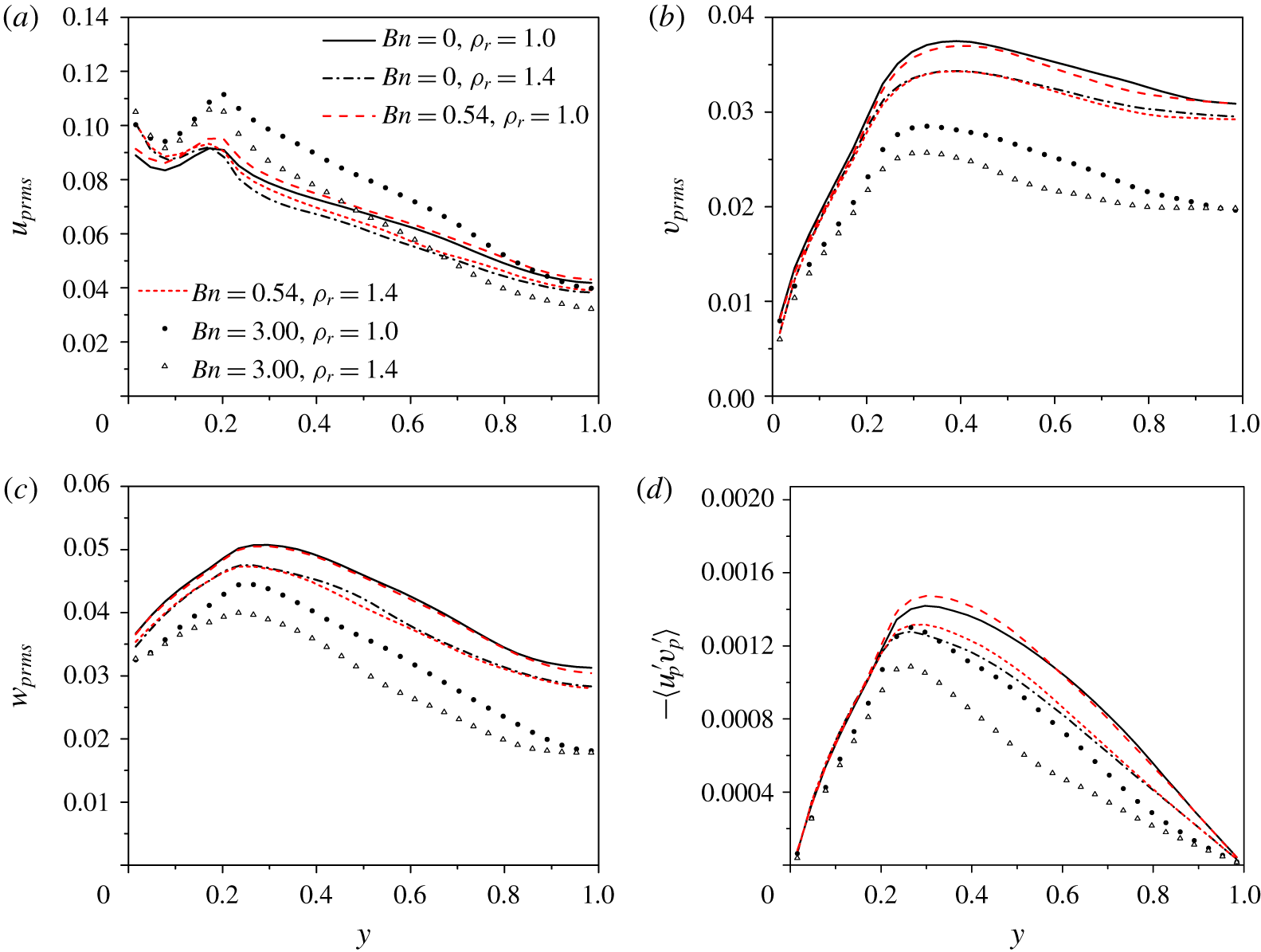
(a–c) Solid-phase r.m.s. velocities: (a) streamwise, (b) transverse and (c) spanwise; and (d) Reynolds shear stress.

The solid-phase r.m.s. velocities and kinematic Reynolds shear stresses (i.e.  $\langle -u_{p}^{\prime }v_{p}^{\prime }\rangle$ without the density) for the particle-laden flows are plotted in figure 19. At the same Bingham number, the intensities of solid-phase velocity fluctuations for the settling particles are lower than for the neutrally buoyant particles, except the streamwise r.m.s. velocity in the near-wall region. The solid-phase r.m.s. velocities are larger than those of the fluid in the near-wall region due to the collisions between the particles and the wall. At the same particle density, the intensities of solid-phase velocity fluctuations generally increase in the streamwise direction and decrease in the transverse and spanwise directions, as the Bingham number increases, which is consistent with the effects of the Bingham number on the fluid-phase velocity fluctuations in figures 13 and 14.
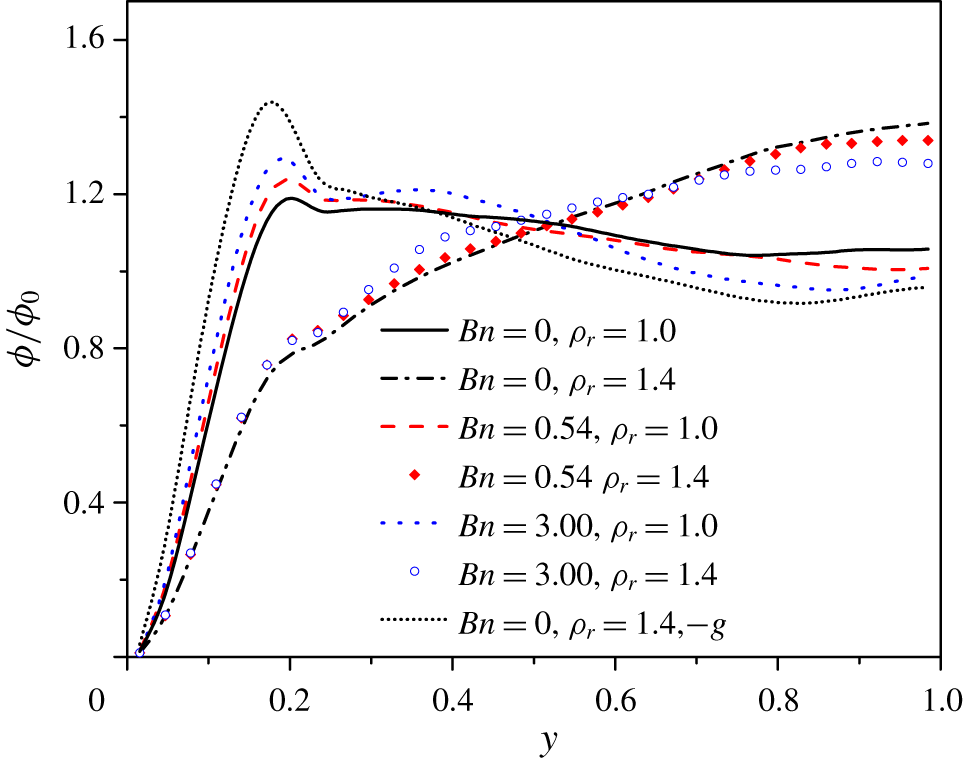
Distribution of the local particle volume fraction normalized by the average particle volume fraction.

Figure 20 shows the distribution of the particle volume fraction normalized by the average particle volume fraction. It is observed that the heavier particles ( $\unicode[STIX]{x1D70C}_{r}=1.4$) tend to migrate towards the channel centreline, as observed in the experiment of Shokri et al. (Reference Shokri, Ghaemi, Nobes and Sanders2017) on the particle-laden flows in a vertical tube, whereas the distributions of the neutrally buoyant particles (
 $\unicode[STIX]{x1D70C}_{r}=1.0$) are roughly homogeneous across the channel, with slightly higher concentrations near the wall. As the Bingham number increases, the particle volume fraction is enhanced near the wall and reduced in the channel centre region. The reason is not clear, and may be related to the variation of the effective viscosity of the Bingham fluid across the channel. For the laminar Poiseuille flow, the Saffman lift force can drive the lagging particle to migrate towards the channel centre and the leading particle to migrate towards the channel wall. We conjecture that the Saffman lift force is responsible for the migration of the heavier particles in figure 20. To confirm this, an extra case with the gravity direction changed to the same as the flow direction is simulated, and the result (dotted line in figure 20) shows that the particles tend to migrate towards the wall, consistent with the direction of the Saffman force. Thus the lateral migration of the particles in turbulence is driven by the Saffman force, and the turbulence causes the diffusion of the particle volume fraction. It is surprising that the migration of the heavier particles is significant for
 $Bn=3.0$, considering that the slip velocity is very small (figure 15b). The lateral migration direction of the heavier particles in the near-wall region is seemingly conflicting with the phase-averaged slip velocity in figure 15. However, it has been shown in figure 18(c) that the heavier particles always tend to lag the local fluid due to the sedimentation effect, and thus the Saffman force does not change its direction across the channel.
There are two differences between the cases for  $\unicode[STIX]{x1D70C}_{r}=1.4$ and 1.0. One is the presence of buoyancy and the other is the higher particle inertia for
 $\unicode[STIX]{x1D70C}_{r}=1.4$, compared with
 $\unicode[STIX]{x1D70C}_{r}=1.0$. Fornari et al. (Reference Fornari, Formenti, Picano and Brandt2016a) showed that the neutrally buoyant particles with
 $\unicode[STIX]{x1D70C}_{r}=2.0$ did not migrate laterally, as for the case of
 $\unicode[STIX]{x1D70C}_{r}=1.0$, although pronounced migration towards the channel centre was observed for
 $\unicode[STIX]{x1D70C}_{r}=10.0$ (Fornari et al. Reference Fornari, Formenti, Picano and Brandt2016a; Yu et al. Reference Yu, Lin, Shao and Wang2017). Therefore, the particle inertia for
 $\unicode[STIX]{x1D70C}_{r}=1.4$ does not cause lateral migration, and the migration observed is due to the particle settling effect.
The lateral migration of the settling particles should be responsible for the turbulence attenuation by the particle settling effect, as observed in figure 14. For  $Bn=3.0$, the particles enhance the turbulence by inducing the vortices near the wall where the shear rate is large, and the enhancement for the settling case is smaller than for the neutrally buoyant case since there are fewer particles located in the near-wall region as a result of the migration of settling particles. The particles in the bulk region seem to attenuate the turbulence, probably by increasing the viscous dissipation.
3.6 Discussion on the flow drag
The friction coefficient is defined as  $C_{f}=2\unicode[STIX]{x1D70F}_{w}/\unicode[STIX]{x1D70C}u_{b}^{2}$, where
 $\unicode[STIX]{x1D70F}_{w}$ is the wall shear stress. Table 2 shows that the friction coefficient decreases with increasing Bingham number, and is largest for the neutrally buoyant particle-laden flow and lowest for the particle-free flow at the same Bingham number. An interesting result is that the particle sedimentation reduces the friction drag, as compared with the neutrally buoyant case. In this subsection, we will explore the reasons for the effects of the particles and the Bingham number on the friction drag. Based on the spatial averaging theorem, the mean momentum equation of turbulent channel flow can be derived as (Picano et al. Reference Picano, Breugem and Brandt2015; Yu et al. Reference Yu, Lin, Shao and Wang2017)
 $$\begin{eqnarray}\displaystyle & & \displaystyle \frac{\text{d}}{\text{d}y}(\unicode[STIX]{x1D711}_{f}\langle \unicode[STIX]{x1D70E}_{f}\rangle _{xy}+\unicode[STIX]{x1D711}_{s}\langle \unicode[STIX]{x1D70E}_{s}\rangle _{xy})+\left(-\frac{\text{d}p_{e}}{\text{d}x}\right)\nonumber\\ \displaystyle & & \displaystyle \quad +\,\frac{\text{d}}{\text{d}y}(\unicode[STIX]{x1D711}_{f}\unicode[STIX]{x1D70C}_{f}\langle -u_{f}^{\prime }v_{f}^{\prime }\rangle +\unicode[STIX]{x1D711}_{s}\unicode[STIX]{x1D70C}_{s}\langle -u_{s}^{\prime }v_{s}^{\prime }\rangle )-\unicode[STIX]{x1D711}_{s}(\unicode[STIX]{x1D70C}_{r}-\unicode[STIX]{x1D70C}_{f})g=0,\end{eqnarray}$$
where  $u$ and
 $v$ are the local velocity components in the
 $x$- and
 $y$-directions, respectively, with the subscript ‘
 $f$’ meaning the fluid phase and ‘
 $s$’ meaning the solid phase,
 $\unicode[STIX]{x1D70E}_{s}$ is the solid inner stress,
 $g$ is the gravity, and
 $\unicode[STIX]{x1D711}_{f}$ and
 $\unicode[STIX]{x1D711}_{s}$ are the fluid and solid volume fractions at a given
 $y$-position. Note that here the particle Reynolds stress means the solid-phase Reynolds stress; namely, the velocities at the Eulerian grids inside the particle boundaries rather than the particle translational velocities are used for the computation of the particle Reynolds stress. For the two-phase vertical channel flow, the relationship between
 $p_{e}$ and
 $\unicode[STIX]{x1D70F}_{w}$ is
 $-\text{d}p_{e}/\text{d}x=\unicode[STIX]{x1D70F}_{w}/H+\unicode[STIX]{x1D711}_{0}(\unicode[STIX]{x1D70C}_{s}-\unicode[STIX]{x1D70C}_{f})g$. Equation (3.3) can be rewritten as follows:
 $$\begin{eqnarray}\displaystyle -\frac{\unicode[STIX]{x1D70F}_{w}}{H} & = & \displaystyle \frac{\text{d}}{\text{d}y}(\unicode[STIX]{x1D711}_{f}\langle \unicode[STIX]{x1D70E}_{f}\rangle _{xy}+\unicode[STIX]{x1D711}_{s}\langle \unicode[STIX]{x1D70E}_{s}\rangle _{xy})+(\unicode[STIX]{x1D711}_{0}-\unicode[STIX]{x1D711}_{s})(\unicode[STIX]{x1D70C}_{r}-\unicode[STIX]{x1D70C}_{f})g\nonumber\\ \displaystyle & & \displaystyle +\,\frac{\text{d}}{\text{d}y}(\unicode[STIX]{x1D711}_{f}\unicode[STIX]{x1D70C}_{f}\langle -u_{f}^{\prime }v_{f}^{\prime }\rangle +\unicode[STIX]{x1D711}_{s}\unicode[STIX]{x1D70C}_{s}\langle -u_{s}^{\prime }v_{s}^{\prime }\rangle ).\end{eqnarray}$$
The contributions of different stresses to the friction coefficient can be obtained by applying triple integration (Fukagata, Iwamoto & Kasagi Reference Fukagata, Iwamoto and Kasagi2002), i.e.  $\int _{0}^{1}\text{d}y\int _{0}^{y}\text{d}y\int _{0}^{y}\text{d}y$, to (3.4) to give
 $$\begin{eqnarray}\displaystyle C_{f} & = & \displaystyle \underbrace{\frac{12}{Re_{b}}\int _{0}^{1}(1-y)\unicode[STIX]{x1D711}_{f}\left(\frac{\text{d}u^{\ast }}{\text{d}y}\right)\text{d}y}_{C_{fV}}+\underbrace{6\int _{0}^{1}(1-y)\unicode[STIX]{x1D711}_{f}\frac{\bar{\unicode[STIX]{x1D706}}_{b12}\unicode[STIX]{x1D70F}_{y}}{\unicode[STIX]{x1D70C}_{f}u_{b}^{2}}\,\text{d}y}_{C_{fy}}\nonumber\\ \displaystyle & & \displaystyle +\,\underbrace{6\int _{0}^{1}(1-y)(\unicode[STIX]{x1D711}_{f}\langle -u_{f}^{\ast \prime }v_{f}^{\ast \prime }\rangle )\,\text{d}y}_{C_{fR}}+\underbrace{6\int _{0}^{1}(1-y)\frac{\unicode[STIX]{x1D711}_{s}}{\unicode[STIX]{x1D70C}_{f}u_{b}^{2}}\langle \unicode[STIX]{x1D70E}_{s}\rangle _{xy}\,\text{d}y}_{Cpi}\nonumber\\ \displaystyle & & \displaystyle +\,\underbrace{6\int _{0}^{1}(1-y)(\unicode[STIX]{x1D711}_{s}\unicode[STIX]{x1D70C}_{r}\langle -u_{s}^{\ast \prime }v_{s}^{\ast \prime }\rangle )\,\text{d}y}_{C_{pR}}+\underbrace{\left(-3\int _{0}^{1}(1-y)^{2}(\unicode[STIX]{x1D711}_{s}-\unicode[STIX]{x1D711}_{0})(\unicode[STIX]{x1D70C}_{s}-1)g^{\ast }\,\text{d}y\right)}_{Cg}.\nonumber\\ \displaystyle & & \displaystyle\end{eqnarray}$$
Here  $C_{f}$ is the friction coefficient defined by
 $C_{f}=2\unicode[STIX]{x1D70F}_{w}/\unicode[STIX]{x1D70C}_{f}u_{b}^{2}$;
 $y$ is the dimensionless coordinate normalized with
 $H$, with the wall position shifted to
 $y=0$;
 $u^{\ast }$ and
 $v^{\ast }$ denote the dimensionless velocities normalized by
 $u_{b}$; and
 $g^{\ast }$ represents
 $g^{\ast }=gH/u_{b}^{2}$, which is actually the Froude number defined in (6). We define the terms of the fluid viscous stress, the yield stress, the fluid Reynolds stress, the particle inner stress, the particle Reynolds stress and the gravity in (3.5) as
 $C_{fV}$,
 $C_{fy}$,
 $C_{fR}$,
 $C_{pi}$,
 $C_{pR}$ and
 $C_{g}$, respectively. To derive (3.5), the following relations are used:
 $$\begin{eqnarray}\displaystyle (\unicode[STIX]{x1D719}_{f}\langle \unicode[STIX]{x1D70E}_{f}\rangle _{xy}+\unicode[STIX]{x1D719}_{s}\langle \unicode[STIX]{x1D70E}_{s}\rangle _{xy})|_{y=0}=\unicode[STIX]{x1D70F}_{w},\end{eqnarray}$$
 $$\begin{eqnarray}\displaystyle \int _{0}^{1}\int _{0}^{y}f\,\text{d}y\,\text{d}y=\int _{0}^{1}(1-y)f\,\text{d}y,\quad \int _{0}^{1}\int _{0}^{y}\int _{0}^{y}f\,\text{d}y\,\text{d}y\,\text{d}y={\textstyle \frac{1}{2}}\int _{0}^{1}(1-y)^{2}f\,\text{d}y.\end{eqnarray}$$
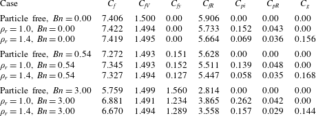
Contributions of the terms in (3.5) to  $C_{f}$ (the data unit is
 $\times 10^{-3}$).

The values of the terms in (3.5) are presented in table 3. From the data, the decrease in the friction coefficient with increasing Bingham number is mainly due to the decrease in the fluid Reynolds-stress term, although the yield-stress term  $C_{fy}$ is larger for a higher Bingham number. The yield stress increases the effective viscosity of the fluid, which increases the flow drag directly, but on the other hand decreases the flow drag indirectly by weakening the turbulence. The decrease in the friction coefficient with increasing Bingham number indicates that the indirect effect of the yield stress prevails over the direct effect. The Bingham fluid is a shear-thinning fluid. The effective viscosity is lower on the wall and higher in the bulk region, which might favour the generation of the drag reduction of the Bingham fluid.
From table 3, the reduction in the friction coefficient by the particle settling effect (i.e.  $\unicode[STIX]{x1D70C}_{s}=1.4$ versus
 $\unicode[STIX]{x1D70C}_{s}=1.0$) is mainly caused by the reduction in fluid Reynolds stress, which overwhelms the additional contribution of the gravity term for the non-neutrally buoyant case. The lateral migration of the settling particles is expected to result in a lower Reynolds stress compared with the neutrally buoyant case, as discussed earlier.
4 Conclusion
We have investigated the effects of the fluid yield stress and the finite-size particles on the turbulent channel flow by using a parallel direct-forcing fictitious domain (DF/FD) method. The main findings are as follows.
(1) As a result of the increase in the apparent viscosity, the single-phase flow for
 $Re_{b}=8000$ and $Bn=3.0$ is in the transitional state, with strong temporal and spatial intermittencies and an asymmetry in the fluid statistics during a long simulation time. The vortices are typically concentrated in the streamwise-extended regions, staggered with the laminar regions in the spanwise direction. The vortex bands in the two half-channels are also typically staggered in the spanwise direction. When the particles are added, the vortices are induced by the particles in the near-wall region, which increases the turbulence and reduces the flow intermittencies greatly.
(2) Particle sedimentation reduces the fluid velocity fluctuations and the friction drag, as compared with the neutrally buoyant case. This is probably caused by the migration of the settling particles towards the channel centre due to the Saffman force: the particles in the near-wall region can enhance the turbulence by inducing vortices, while the particles in the bulk region may weaken the turbulence by increasing the viscous dissipation.
(3) As the Bingham number increases, the friction drag decreases, mainly due to the attenuation in the fluid Reynolds stress, accompanied by the increase in the streamwise r.m.s. velocity, and the decrease in the transverse and spanwise r.m.s. velocities.


The computational cost for the Bingham fluid case is around 20 times that for the Newtonian fluid case, due to the large number of iterations for the solution of the plasticity subproblem (2.27)–(2.28). Therefore, we cannot employ a finer grid than  $512\times 128\times 256$. Only weak particle settling effects and large particles are considered in the present study, because of the huge computational cost for the Bingham fluid. This is a good subject for future study to investigate the cases of relatively strong particle sedimentation and relatively small particles.
Acknowledgements
The work was supported by the National Natural Science Foundation of China (grant nos 91752117, 91852204 and 11632016).