1 Introduction
This paper is a sequel to [Reference Lehrer and Zhang19] and [Reference Deligne, Lehrer and Zhang6], in which we proved the first fundamental theorem (FFT) of invariant theory for the orthosymplectic group superscheme  $G=\text{OSp}(m|2n,\mathbb{C})$. The FFT may be interpreted either in terms of the group superscheme
 $G=\text{OSp}(m|2n,\mathbb{C})$ or in terms of the points
 $G(\unicode[STIX]{x1D6EC})$ of
 $G$ over the infinite dimensional Grassmann algebra
 $\unicode[STIX]{x1D6EC}$, which form an actual group of matrices over
 $\unicode[STIX]{x1D6EC}$. In this work, we adopt the scheme-theoretic point of view of [Reference Deligne, Lehrer and Zhang6]. The FFT provides a set of generators for the invariants of
 $G$ on
 $V^{\otimes r}$, where
 $V$ is the “natural” representation of
 $G$ on the superspace
 $V$ of superdimension
 $(m|2n)$; this theorem is equivalent to the statement that there is a surjection
 ${\mathcal{B}}_{r}(m-2n)\longrightarrow \text{End}_{G}(V^{\otimes r})$, where
 ${\mathcal{B}}_{r}(m-2n)$ is the
 $r$-string Brauer algebra with parameter
 $m-2n$. In this paper, we give a linear description of all relations among these generators; this is the second fundamental theorem (SFT) of invariant theory.
The thrust of the geometric approach we use is to reduce the questions concerning  $\text{OSp}(m|2n,\mathbb{C})$ to similar questions concerning the action of
 $\text{GL}(m|2n,\mathbb{C})$ on a larger space. In this work, we show that this reduction may be performed so as to throw light on the SFT for
 $\text{OSp}(m|2n,\mathbb{C})$ using a combination of geometric and diagrammatic methods.
In this section, we briefly recall the results of [Reference Deligne, Lehrer and Zhang6, Reference Lehrer and Zhang19] in a form convenient for the present exposition.
1.1 Superalgebraic geometry
We refer to [Reference Deligne, Lehrer and Zhang6, Section 2] for the basic facts concerning superschemes. We shall work in the category of superschemes over the complex field  $\mathbb{C}$. Each such superscheme
 $S$ gives rise to a functor on the category of (super) commutative
 $\mathbb{C}$-superalgebras
 $$\begin{eqnarray}S:A\mapsto S(A):=\text{Hom}(\text{Spec}(A),S),\end{eqnarray}$$
which takes the superalgebra  $A$ to the set of
 $A$-points of
 $S$. This is the functor of points associated with
 $S$ with which we identify
 $S$. We shall use the term “function” on a superscheme
 $S$ to mean a global section of the structure sheaf
 ${\mathcal{O}}={\mathcal{O}}_{S}$ of
 $S$.
If  $W_{\mathbb{C}}$ is a finite dimensional complex superspace, one associates to it the superscheme
 $W=\text{Spec}(S(W_{\mathbb{C}}^{\ast }))$, whose corresponding functor of points
 ${\mathcal{W}}$ takes a supercommutative superalgebra
 $A$ to
 ${\mathcal{W}}(A):=(W\otimes _{\mathbb{C}}A)_{\bar{0}}$. In the special case
 $W_{\mathbb{C}}=\mathbb{C}$ (even), the corresponding superscheme is denoted as
 $\mathbb{G}_{a}$. When
 $W_{\mathbb{C}}$ has an extra structure, for example, if it is a
 $\mathbb{C}$-algebra, the scheme
 $W$ will inherit that structure. Thus,
 $\mathbb{G}_{a}$ is an additive group.
Given an action of an affine supergroup  $G$ over
 $\mathbb{C}$ on a (complex) supervector space
 $W$, for any supercommutative superalgebra
 $A$,
 $G(A)$ acts on
 $W\otimes _{\mathbb{C}}A$.
Definition 1.1. A vector  $w\in W$ is said to be invariant under
 $G$ if for any
 $A$,
 $w\otimes 1$ is fixed by each element of
 $G(A)$. Denote the space of invariants by
 $W^{G}$. This is a vector subspace of
 $W$.
Equivalently, in the language of Hopf algebras, if  $F(G)$ is the coordinate superalgebra of
 $G$ (so
 $G=\text{Spec}(F(G))$), we have the coaction
 $W\rightarrow W\otimes F(G)$ as well as the map
 $w\mapsto w\otimes 1\in W\otimes F(G)$. Then
 $W^{G}=\text{Ker}(W\rightrightarrows W\otimes F(G))$.
If the functor of points associated with the fixed point space  $W^{G}$ is written
 ${\mathcal{W}}^{G}$, then for any supercommutative superalgebra
 $A$, we have
 ${\mathcal{W}}^{G}(A)=\left((W\otimes _{\mathbb{C}}A)^{G(A)}\right)_{\bar{0}}$.
1.2 Linear superalgebra and the group scheme  $\text{GL}(V)$

See [Reference Lehrer and Zhang19, Sections 2.1, 2.2]. We denote by  $V=(V)_{\bar{0}}\oplus (V)_{\bar{1}}$ a
 $\mathbb{Z}/2\mathbb{Z}$-graded complex vector space of superdimension
 $\text{sdim }V=(m|2n)$ so that
 $\dim (V)_{\bar{0}}=m$ and
 $\dim (V)_{\bar{1}}=2n$. The supersymmetric algebra
 $S(V^{\ast })$ is the supercommutative super
 $\mathbb{C}$-algebra defined in [Reference Lehrer and Zhang19, Section 3.2], and the scheme
 ${\mathcal{V}}$ corresponding to
 $V$ is
 ${\mathcal{V}}:=\text{Spec}(S(V^{\ast }))$. Its associated functor of points is described above.
As a special case, we have the affine superscheme  ${\mathcal{E}}nd(V)$ of endomorphisms of
 $V$, which is associated with the supervector space
 $\text{End}(V):=\text{End}_{\mathbb{C}}(V)$; it has the open subscheme
 $\text{GL}(V)$ (see [Reference Deligne, Lehrer and Zhang6, 2.10]) whose associated functor of points takes the supercommutative superalgebra
 $A$ to
 $\text{Aut}_{A}(V\otimes _{\mathbb{C}}A)$.
1.3 The orthosymplectic supergroup $\text{OSp}(V)$

Consider a nondegenerate even bilinear form
 $$\begin{eqnarray}\displaystyle B:=(-,-):V\times V\longrightarrow \mathbb{C}, & & \displaystyle\end{eqnarray}$$
which is supersymmetric, that is,  $(u,v)=(-1)^{[u][v]}(v,u)$ for all
 $u,v\in V$. This implies that the form is symmetric on
 $(V)_{\bar{0}}\times (V)_{\bar{0}}$, skew symmetric on
 $(V)_{\bar{1}}\times (V)_{\bar{1}}$, and satisfies
 $(V_{\bar{0}},V_{\bar{1}})=0=(V_{\bar{1}},V_{\bar{0}})$. Also, by nondegeneracy,
 $\dim (V)_{\bar{1}}=2n$ must be even. We call this a nondegenerate supersymmetric form on
 $V$. Let
 $\unicode[STIX]{x1D702}=\left(\begin{array}{@{}cc@{}}I_{m} & 0\\ 0 & J_{n}\end{array}\right),$ where
 $I_{m}$ is the identity matrix of size
 $m\times m$ and
 $J_{n}$ is a skew symmetric matrix of size
 $2n\times 2n$ given by
 $J_{n}=\text{diag}(\unicode[STIX]{x1D70E},\ldots ,\unicode[STIX]{x1D70E})$ with
 $\unicode[STIX]{x1D70E}=\left(\begin{array}{@{}cc@{}}0 & -1\\ 1 & 0\end{array}\right)$. Then there exists an ordered homogeneous basis
 ${\mathcal{E}}=(e_{1},e_{2},\ldots ,e_{m+2n})$ of
 $V$ such that
 $$\begin{eqnarray}\displaystyle (e_{a},e_{b})=\unicode[STIX]{x1D702}_{ab},\quad \text{for all }a,b. & & \displaystyle\end{eqnarray}$$
As in [Reference Deligne, Lehrer and Zhang6, Example 2.6], the form  $(-,-)$ gives rise to a bilinear morphism of functors
 $$\begin{eqnarray}\displaystyle B:{\mathcal{V}}\times {\mathcal{V}}\rightarrow \mathbb{G}_{a}, & & \displaystyle\end{eqnarray}$$
which corresponds (cf. [Reference Deligne, Lehrer and Zhang6, Section 2.7]) to a quadratic form  $q\in S^{2}(V)_{\bar{0}}$, which is related to
 $B$ via
 $$\begin{eqnarray}\displaystyle \begin{array}{@{}rcl@{}}q(x)\; & =\; & {\textstyle \frac{1}{2}}B(x,x)\qquad \text{and}\\ B(x,y)\; & =\; & q(x+y)-q(x)-q(y).\end{array} & & \displaystyle\end{eqnarray}$$
Definition 1.2. [Reference Deligne, Lehrer and Zhang6, 2.11]
The orthosymplectic group superscheme  $G=\text{OSp}(V)$ is defined as the subscheme of
 $\text{GL}(V)$ which preserves the form
 $B(-,-)$ or, equivalently, which preserves the quadratic form
 $q$. Explicitly,
 $G=\{g\in \text{GL}(V)\mid q\circ g^{-1}=q\}$.
An  $A$-point of the group scheme corresponding to
 $\text{OSp}(V)$ is an automorphism of
 $V\otimes _{\mathbb{C}}A$ which fixes the
 $A$-bilinear form induced on
 $V\otimes _{\mathbb{C}}A$ by
 $B(-,-)$.
2 Invariant theory for $\text{GL}(V)$

In this section, we state the two fundamental theorems of invariant theory for the supergroup  $\text{GL}(m|\ell )$ in a form convenient for use in our context.
2.1 Symmetric group action
In this section, we take  $V$ to be a
 $\mathbb{C}$-superspace with
 $\text{sdim }(V)=(m|\ell )$ and, as above, write
 ${\mathcal{V}}$ for the corresponding (super) scheme whose associated functor of points is described above. Given any two
 $\mathbb{Z}_{2}$-graded
 $\mathbb{C}$-vector spaces,
 $V,W$, we may form the tensor product
 $V\otimes _{\mathbb{C}}W$ and
 $\text{Hom}_{\mathbb{C}}(V,W)$. These are
 $\mathbb{Z}_{2}$-graded in the usual way. Thus,
 $\text{GL}(V)$ acts on the superspaces
 $V^{\otimes r}$ for
 $r=1,2,\ldots$. We have a superpermutation
 $\unicode[STIX]{x1D70F}:V\otimes W\longrightarrow W\otimes V$, given by
 $$\begin{eqnarray}\displaystyle \unicode[STIX]{x1D70F}(v\otimes w)=(-1)^{[v][w]}w\otimes v, & & \displaystyle\end{eqnarray}$$
for homogeneous  $v\in V,w\in W$, and extended linearly. When
 $V=W$,
 $\unicode[STIX]{x1D70F}\in \text{End}_{\text{GL}(V)}(V\otimes V)=(\text{End}_{\mathbb{C}}(V\otimes V))^{\text{GL}(V)}$.
Bearing in mind the definition of invariants in Definition 1.1, for any  $r$, we have a homomorphism of
 $\mathbb{C}$-algebras
 $$\begin{eqnarray}\displaystyle \unicode[STIX]{x1D71B}_{r}:\mathbb{C}\text{Sym}_{r}\longrightarrow \text{End}(V^{\otimes r})^{\text{GL}(V)}, & & \displaystyle\end{eqnarray}$$
in which the simple transpositions in  $\text{Sym}_{r}$ are mapped to the endomorphisms
 $\unicode[STIX]{x1D70F}$ of (2.1), acting on the appropriate factors of the product.
Since our strategy for studying  $\text{OSp}(V)$ is to reduce to the case of
 $\text{GL}(V)$, we next state the fundamental theorems for
 $\text{GL}(V)$.
2.2 Invariant theory for $\text{GL}(V)$: the FFT

The FFT for  $\text{GL}(V)$ may be stated as follows.
Theorem 2.1. [Reference Berele and Regev4, Theorems 3.3 and 3.7]
The map  $\unicode[STIX]{x1D71B}_{r}$ of (2.2) is surjective for all
 $r$.
This theorem can be proved in similar manner to the classical case using the superpolarisation result in Appendix A.
Now for any pair of complex vector spaces  $V,W$, the canonical isomorphism
 $$\begin{eqnarray}\displaystyle \text{Hom}_{\mathbb{C}}(V,W)\overset{{\sim}}{\longrightarrow }\text{Hom}_{\mathbb{C}}(V\otimes _{\mathbb{C}}W^{\ast },\mathbb{C}) & & \displaystyle\end{eqnarray}$$
of supervector spaces is  $\text{GL}(V)$-equivariant. Hence, we have the following reformulation of Theorem 2.1. First, observe that the element
 $$\begin{eqnarray}\displaystyle \unicode[STIX]{x1D706}_{0}:(v_{1},\ldots ,v_{r},\unicode[STIX]{x1D719}_{1},\ldots ,\unicode[STIX]{x1D719}_{r})\mapsto \unicode[STIX]{x1D719}_{1}(v_{1})\unicode[STIX]{x1D719}_{2}(v_{2})\cdots \unicode[STIX]{x1D719}_{r}(v_{r}) & & \displaystyle\end{eqnarray}$$
lies in  $(\text{Hom}(V^{\otimes r}\otimes (V^{\ast })^{\otimes r},\mathbb{C}))^{\text{GL}(V)}$; that is, it is invariant according to Definition 1.1.
Next, note that  $\text{Sym}_{r}$ acts on
 $\text{Hom}(V^{\otimes r}\otimes (V^{\ast })^{\otimes s},\mathbb{C})$ via the map
 $\unicode[STIX]{x1D706}\mapsto \unicode[STIX]{x1D70B}(\unicode[STIX]{x1D706}):=\unicode[STIX]{x1D706}\circ (\unicode[STIX]{x1D71B}_{r}(\unicode[STIX]{x1D70B}^{-1})\times \text{id}_{(V^{\ast })^{\otimes s}})$ (for
 $\unicode[STIX]{x1D706}\in \text{Hom}(V^{\otimes r}\otimes (V^{\ast })^{\otimes s},\mathbb{C})$ and
 $\unicode[STIX]{x1D70B}\in \text{Sym}_{r}$).
For  $\unicode[STIX]{x1D70B}\in \text{Sym}_{r}$, let
 $\unicode[STIX]{x1D6FF}_{\unicode[STIX]{x1D70B}}=\unicode[STIX]{x1D70B}(\unicode[STIX]{x1D706}_{0})\in \text{Hom}(V^{\otimes r}\otimes (V^{\ast })^{\otimes r},\mathbb{C})$. Thus, for homogeneous
 $v_{1},\ldots ,v_{r},\unicode[STIX]{x1D719}_{1},\ldots ,\unicode[STIX]{x1D719}_{r}$,
 $$\begin{eqnarray}\displaystyle \unicode[STIX]{x1D6FF}_{\unicode[STIX]{x1D70B}}(v_{1},\ldots ,v_{r},\unicode[STIX]{x1D719}_{1},\ldots ,\unicode[STIX]{x1D719}_{r})=\pm \mathop{\prod }_{i=1}^{r}\unicode[STIX]{x1D719}_{i}(v_{\unicode[STIX]{x1D70B}(i)}). & & \displaystyle\end{eqnarray}$$
Corollary 2.2. We have
 $$\begin{eqnarray}\displaystyle \qquad \quad \text{Hom}(V^{\otimes r}\otimes (V^{\ast })^{\otimes s},\mathbb{C})^{\text{GL}(V)}=\left\{\begin{array}{@{}ll@{}}0\quad & \text{if }r\neq s\\ \text{span}\;\{\unicode[STIX]{x1D6FF}_{\unicode[STIX]{x1D70B}}\mid \unicode[STIX]{x1D70B}\in \text{Sym}_{r}\}\quad & \text{if }r=s.\end{array}\right. & & \displaystyle\end{eqnarray}$$
The first statement is trivial since the center of  $\text{GL}(V)$ is just
 $\mathbb{C}$ and
 $z\in \mathbb{C}$ acts on
 $\text{Hom}(V^{\otimes r}\otimes (V^{\ast })^{\otimes s},\mathbb{C})$ as multiplication by
 $z^{r-s}$. The second statement is easily seen to be equivalent to Theorem 2.1.
2.3 Invariant theory for $\text{GL}(V)$: the SFT

The SFT for  $\text{GL}(V)$ describes the kernel of the surjective homomorphism
 $\unicode[STIX]{x1D71B}_{r}$ of Theorem 2.1.
The following result is an easy consequence of [Reference Berele and Regev4, Theorem 3.20].
Theorem 2.3. Let  $V$ be a super
 $\mathbb{C}$-vector space with
 $\text{sdim }(V)=m|\ell$. If
 $r<(m+1)(\ell +1)$, then the surjective (by Theorem 2.1) homomorphism
 $$\begin{eqnarray}\unicode[STIX]{x1D71B}_{r}:\mathbb{C}\text{Sym}_{r}\longrightarrow \left(\text{End}_{\mathbb{C}}(V)^{\otimes r}\right)^{\text{GL}(V)}\end{eqnarray}$$
of superalgebras is an isomorphism. If  $r\geqslant (m+1)(\ell +1)$, then the kernel of
 $\unicode[STIX]{x1D71B}_{r}$ is the (two-sided) ideal of
 $A\text{Sym}_{r}$ generated by the Young symmetrizer of the partition with
 $m+1$ rows and
 $\ell +1$ columns.
The kernel is therefore generated by an idempotent which is explicitly described as follows. Consider the  $(m+1)\times (\ell +1)$ array of integers below, which form a standard tableau.

Let  $R$ and
 $C$ be the subgroups of
 $\text{Sym}_{m\ell +m+\ell +1}$ (regarded as the subgroup of
 $\text{Sym}_{r}$ which permutes the first
 $(m+1)(\ell +1)$ numbers) which stabilize the rows and columns of the array, respectively. Thus,
 $$\begin{eqnarray}\displaystyle R & = & \displaystyle \text{Sym}\{1,2,\ldots ,\ell +1\}\times \text{Sym}\{\ell +2,\ell +3,\ldots ,2\ell +2\}\times \cdots \nonumber\\ \displaystyle & & \displaystyle \cdots \times \text{Sym}\{m\ell +m+1,m\ell +m+2,\ldots ,m\ell +m+\ell +1\},\nonumber\end{eqnarray}$$
while
 $$\begin{eqnarray}\displaystyle C & = & \displaystyle \text{Sym}\{1,\ell +2,\ldots ,m\ell +m+1\}\times \text{Sym}\{2,\ell +3,\ldots ,m\ell +m+2\}\times \cdots \nonumber\\ \displaystyle & & \displaystyle \cdots \times \text{Sym}\{\ell +1,2\ell +2,\ldots ,m\ell +m+\ell +1\},\nonumber\end{eqnarray}$$
where  $\text{Sym}\{X\}$ denotes the group of permutations of the finite set
 $X$.
Then in the group ring  $A\text{Sym}_{m\ell +m+\ell +1}\subseteq A\text{Sym}_{r}$, let
 $e=e(m,\ell )$ be the (even) element defined by
 $$\begin{eqnarray}\displaystyle e(m,\ell )=\left(\mathop{\sum }_{\unicode[STIX]{x1D70B}\in R}\unicode[STIX]{x1D70B}\right)\left(\mathop{\sum }_{\unicode[STIX]{x1D70E}\in C}\unicode[STIX]{x1D700}(\unicode[STIX]{x1D70E})\unicode[STIX]{x1D70E}\right)=\unicode[STIX]{x1D6FC}^{+}(R)\unicode[STIX]{x1D6FC}^{-}(C), & & \displaystyle\end{eqnarray}$$
where  $\unicode[STIX]{x1D700}$ is the sign character of
 $\text{Sym}_{r}$, and for any subset
 $H\subseteq \text{Sym}_{r}$, we write
 $\unicode[STIX]{x1D6FC}^{+}(H)$ (resp.
 $\unicode[STIX]{x1D6FC}^{-}(H)$) for the element
 $\sum _{h\in H}h$ (resp.
 $\sum _{h\in H}\unicode[STIX]{x1D700}(h)h$) of
 $\mathbb{C}\text{Sym}_{r}$.
It is known that  $(|R|!|C|!)^{-1}e(m,\ell )$ is a primitive idempotent in the group algebra
 $\mathbb{C}\text{Sym}_{m\ell +m+\ell +1}$. It is also well known that
 $\mathbb{C}\text{Sym}_{r}=\bigoplus _{\unicode[STIX]{x1D707}}I(\unicode[STIX]{x1D707})$, where
 $\unicode[STIX]{x1D707}$ runs over the partitions of
 $r$, and
 $I(\unicode[STIX]{x1D707})$ is a simple ideal of
 $\mathbb{C}\text{Sym}_{r}$ for each
 $\unicode[STIX]{x1D707}$. In this notation, the ideal
 $I(m,\ell )$ of
 $\mathbb{C}\text{Sym}_{r}$ which is generated by
 $e(m,\ell )$ is the sum of the
 $I(\unicode[STIX]{x1D707})$ over those partitions
 $\unicode[STIX]{x1D707}$ that contain an
 $(m+1)\times (\ell +1)$ rectangle.
Corollary 2.4. If  $r<(m+1)(\ell +1)$, then
 $\text{Ker}(\unicode[STIX]{x1D71B}_{r})=0$. Otherwise,
 $\text{Ker}(\unicode[STIX]{x1D71B}_{r})=I(m,\ell ):=\bigoplus _{\unicode[STIX]{x1D707}}I(\unicode[STIX]{x1D707})$ over those partitions
 $\unicode[STIX]{x1D707}$ of
 $r$ that contain a rectangle of size
 $(m+1)\times (\ell +1)$.
2.4 The SFT for $\text{GL}(V)$: second formulation

We shall now translate the FFT for  $\text{GL}(V)$ into the setting of Corollary 2.2. This is easily achieved by noting the commutativity of the following diagram (2.4):

Here,  $\unicode[STIX]{x1D71B}_{r}$ is as in (2.2),
 $\unicode[STIX]{x1D719}_{r,r}$ is a special case of the map in (2.3), and
 $\unicode[STIX]{x1D6FF}$ is the map taking
 $\unicode[STIX]{x1D70B}\in \text{Sym}_{r}$ to the
 $\unicode[STIX]{x1D6FF}_{\unicode[STIX]{x1D70B}}=\unicode[STIX]{x1D70B}(\unicode[STIX]{x1D706}_{0})$ of (2.5).
Since  $\unicode[STIX]{x1D719}_{r,r}$ is an isomorphism, it follows that
 $\text{Ker}(\unicode[STIX]{x1D71B}_{r})=\text{Ker}(\unicode[STIX]{x1D6FF})$. The following statement is therefore evident.
Corollary 2.5. If  $\unicode[STIX]{x1D6FF}_{\unicode[STIX]{x1D70B}}$ (
 $\unicode[STIX]{x1D70B}\in \text{Sym}_{r}$) is as in (2.5), then for any elements
 $a_{\unicode[STIX]{x1D70B}}\in \mathbb{C}$,
 $\sum _{\unicode[STIX]{x1D70B}\in \text{Sym}_{r}}a_{\unicode[STIX]{x1D70B}}\unicode[STIX]{x1D6FF}_{\unicode[STIX]{x1D70B}}=0$ if and only if
 $\sum _{\unicode[STIX]{x1D70B}\in \text{Sym}_{r}}a_{\unicode[STIX]{x1D70B}}\unicode[STIX]{x1D70B}$ lies in the ideal
 $I(m,\ell )$ of
 $\mathbb{C}\text{Sym}_{r}$. In particular,
 $\text{Ker}(\unicode[STIX]{x1D6FF})=0$ if
 $r<(m+1)(\ell +1)$.
3 Invariant theory for the orthosymplectic supergroup
In this section, we take  $\ell =2n$ and
 $G$ to be the orthosymplectic group scheme
 $G=\text{OSp}(V)\subseteq \text{GL}(V)$ as in Definition 1.2. Clearly,
 $G$ acts on
 $V^{\otimes r}$, and
 $\text{End}_{G}(V^{\otimes r})=\text{End}(V^{\otimes r})^{G}$ is a finite dimensional associative algebra which contains
 $\text{End}(V^{\otimes r})^{\text{GL}(V)}$. One formulation of the FFT for
 $\text{OSp}(V)$, which is proved in [Reference Deligne, Lehrer and Zhang6, Reference Lehrer and Zhang19], describes this algebra. The most convenient formulation of the FFT for
 $\text{OSp}(V)$ is through the Brauer category.
3.1 The Brauer category and FFT for $\text{OSp}(V)$

Let  ${\mathcal{B}}={\mathcal{B}}(m-2n)$ be the Brauer category over
 $\mathbb{C}$ with parameter
 $m-2n$ (see [Reference Lehrer and Zhang18]). This has objects
 $\mathbb{N}=\{0,1,2,3,\ldots \}$ and morphisms
 $\text{Hom}_{{\mathcal{B}}}(s,t):={\mathcal{B}}_{s}^{t}$, the linear span of all Brauer diagrams from
 $s$ to
 $t$ (
 $s,t\in \mathbb{N}$). Recall that the category is generated by the four morphisms depicted below:

These will be denoted, respectively, by  $I,X,A$, and
 $U$, and they belong to
 ${\mathcal{B}}_{1}^{1},{\mathcal{B}}_{2}^{2}$,
 ${\mathcal{B}}_{2}^{0}$, and
 ${\mathcal{B}}_{0}^{2}$, respectively.
Let  $(e_{a}),(e_{a}^{\ast })$ (
 $a=1,2,\ldots ,m+2n$) be a pair of
 $\mathbb{C}$-bases of
 $V$, which are dual with respect to the form
 $B$ in the sense that
 $B(e_{a}^{\ast },e_{b})=\unicode[STIX]{x1D6FF}_{ab}$ (the Kronecker delta) for all
 $a,b$. The element
 $c_{0}=\sum _{a}e_{a}\otimes e_{a}^{\ast }\in V\otimes V$ is then independent of the basis chosen and is
 $G$-invariant.
The FFT for  $\text{OSp}(V)$ may now be stated as follows (cf. [Reference Lehrer and Zhang18, Theorem 4.8]).
Theorem 3.1. Let  $V=\mathbb{C}^{m|2n}$ and
 $G=\text{OSp}(V)$, and let
 ${\mathcal{T}}_{G}$ be the full subcategory of
 $G$-modules with objects
 $V^{\otimes r}$ (
 $r=0,1,2,\ldots$). Then there is a full functor
 $F:{\mathcal{B}}(m-2n)\rightarrow {\mathcal{T}}_{G}$, defined by
 $F(r)=V^{\otimes r}$,
 $F(I)=\text{id}_{V}$,
 $F(X)=\unicode[STIX]{x1D70F}\in \text{End}(V\otimes V)$, and
 $F(A)=B(-,-):v\otimes V\rightarrow \mathbb{C}$, and
 $F(U)=\unicode[STIX]{x1D6FE}$ is the map defined by
 $\unicode[STIX]{x1D6FE}(1)=c_{0}$.
Remark 3.2. Recall that since  $-\text{id}_{V}\in \text{OSp}(V)$ and acts on
 $V^{\otimes r}$ as
 $(-1)^{r}$, it follows that
 $\text{Hom}_{G}(V^{\otimes t},V^{\otimes s})=0$ if
 $s\not \equiv t$ (mod
 $2$) because any element
 $\unicode[STIX]{x1D6FC}\in \text{Hom}_{G}(V^{\otimes t},V^{\otimes s})$ would satisfy
 $\unicode[STIX]{x1D6FC}=-\unicode[STIX]{x1D6FC}$ since it commutes with
 $-\text{id}_{V}$.
Thus, to say that  $F$ is full means that it induces surjections on the respective
 $\text{Hom}$ spaces, that is, it means that the maps
 $F_{t}^{s}:{\mathcal{B}}_{t}^{s}\longrightarrow \text{Hom}_{G}(V^{\otimes t},V^{\otimes s})$ are surjective for all
 $t,s\in \mathbb{N}$ such that
 $s\equiv t$ (mod
 $2$). Since the
 $\text{Hom}$ spaces are (linearly) isomorphic for each
 $t,s$ such that
 $s+t=2r$ (
 $r\in \mathbb{N}$ constant), this surjectivity is equivalent to the corresponding statement for any particular pair
 $t,s$ with
 $t+s=2r$; common choices are
 $s=t=r$ and
 $t=2r$,
 $s=0$, and we give those formulations now. Taking
 $s=t=r$, we obtain the following statement.
Theorem 3.3. [Reference Lehrer and Zhang19, Theorem 5.4]
Let  ${\mathcal{B}}_{r}(m-2n)$ be the Brauer algebra on
 $r$ strings with parameter
 $m-2n$ and generators
 $s_{i},e_{i}$ for
 $i=1,\ldots ,r-1$ (see [Reference Lehrer and Zhang19, Section 5.2]). Then there is a surjective homomorphism
 ${\mathcal{B}}_{r}(m-2n)\longrightarrow \text{End}_{G}(V^{\otimes r})$ such that
 $s_{i}\mapsto \unicode[STIX]{x1D71B}_{r}(s_{i})$ and
 $e_{i}\mapsto \unicode[STIX]{x1D6FE}_{i}$ for all
 $i$, where
 $\unicode[STIX]{x1D6FE}_{i}=\underbrace{\text{id}_{V}\otimes \cdots \otimes \text{id}_{V}}_{i-1}\otimes \unicode[STIX]{x1D6FE}\otimes \underbrace{\text{id}_{V}\otimes \cdots \otimes \text{id}_{V}}_{r-i-1}$, and
 $\unicode[STIX]{x1D6FE}\in \text{End}_{G}(V^{\otimes 2})$ takes
 $v\otimes w$ to
 $B(v,w)c_{0}$, that is,
 $\unicode[STIX]{x1D6FE}=F(U)\circ F(A)$.
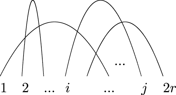
To state the FFT for the case  $t=2r,s=0$, recall that a typical diagram in
 ${\mathcal{B}}_{2r}^{0}$ is of the form depicted in Figure 1.
Diagram  $D:2r\longrightarrow 0$.

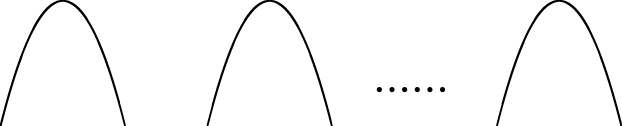
The diagram  $D$ may be obtained from
 $D_{0}$, depicted in Figure 2, by composition with a permutation.
Diagram  $D_{0}:2r\rightarrow 0$.

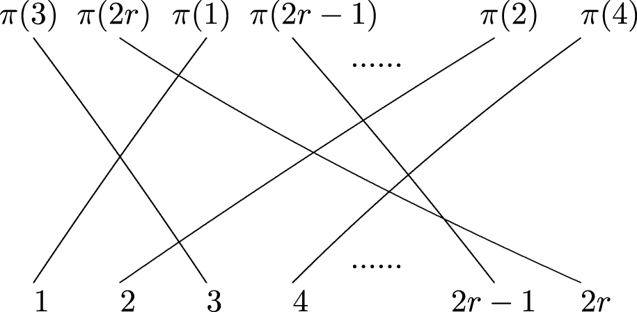
Indeed, any permutation  $\unicode[STIX]{x1D70B}:2r\rightarrow 2r$ may be thought of as a diagram like the one depicted in Figure 3.
Permutation  $\unicode[STIX]{x1D70B}:2r\rightarrow 2r$.

The right action of  $\text{Sym}_{2r}$ on diagrams
 $2r\rightarrow 0$ is then given in terms of diagrams by composition of the diagrams in Figures 1 and 3. It is then clear that any diagram
 $D:2r\rightarrow 0$ may be obtained from the diagram
 $D_{0}$ depicted in Figure 2 by composition with a permutation
 $\unicode[STIX]{x1D70B}\in \text{Sym}_{2r}$ (see Figure 4).
Diagram  $D$ in Figure 1 as composition
 $D_{0}\unicode[STIX]{x1D70B}_{D}$.

To identify the linear maps defined by the diagrams above, define  $\unicode[STIX]{x1D705}_{0}:V^{\otimes 2r}\longrightarrow \mathbb{C}$ by
 $$\begin{eqnarray}\displaystyle \unicode[STIX]{x1D705}_{0}(v_{1}\otimes \cdots \otimes v_{2r})=B(v_{1},v_{2})B(v_{3},v_{3})\ldots B(v_{2r-1},v_{2r}). & & \displaystyle\end{eqnarray}$$
For each permutation  $\unicode[STIX]{x1D70B}\in \text{Sym}_{2r}$, define
 $$\begin{eqnarray}\displaystyle \unicode[STIX]{x1D705}_{\unicode[STIX]{x1D70B}}(v_{1}\otimes \cdots \otimes v_{2r})=\unicode[STIX]{x1D705}_{0}\circ \unicode[STIX]{x1D71B}_{2r}(\unicode[STIX]{x1D70B}^{-1})(v_{1}\otimes \cdots \otimes v_{2r}). & & \displaystyle\end{eqnarray}$$
It is then easily verified that given a diagram  $D\in {\mathcal{B}}_{2r}^{0}$, if
 $D=D_{0}\circ \unicode[STIX]{x1D70B}$ (for
 $\unicode[STIX]{x1D70B}\in \text{Sym}_{2r}$), then although
 $\unicode[STIX]{x1D70B}$ is not uniquely defined by this property,
 $\unicode[STIX]{x1D705}_{\unicode[STIX]{x1D70B}}$ depends only on
 $D$. We therefore write
 $\unicode[STIX]{x1D705}_{\unicode[STIX]{x1D70B}}=\unicode[STIX]{x1D705}_{D}$, and we have the following formulation of the FFT.
Theorem 3.4. Let  $V=\mathbb{C}^{m|2n}$ and
 $G=\text{OSp}(V)$. Then for each integer
 $r$, we have a surjective map
 $\unicode[STIX]{x1D705}:{\mathcal{B}}_{2r}^{0}\longrightarrow \text{Hom}_{G}(V^{\otimes 2r},\mathbb{C})$ which takes the diagram
 $D$ in Figure 1 to
 $\unicode[STIX]{x1D705}_{D}$.
Definition 3.5. Define the subgroup  $C\subseteq \text{Sym}_{2r}$ as the stabilizer of
 $\unicode[STIX]{x1D705}_{0}$ in
 $\text{Sym}_{2r}$. That is,
 $C:=\{\unicode[STIX]{x1D70B}\in \text{Sym}_{2r}\mid \unicode[STIX]{x1D705}_{\unicode[STIX]{x1D70B}}=\unicode[STIX]{x1D705}_{0}\}$.
The idempotent  $e(C)\in \mathbb{C}\text{Sym}_{2r}$ is defined by
 $e(C)=|C|^{-1}\sum _{\unicode[STIX]{x1D70B}\in C}\unicode[STIX]{x1D70B}$.
It is clear that  $|C|=2^{r}r!$ so that
 $|\text{Sym}_{2r}/C|=\prod _{i=1}^{r}(2i-1)=|{\mathcal{B}}_{2r}^{0}|$.
4 From invariants of $\text{OSp}(V)$ to invariants of $\text{GL}(V)$


In this section, we recall the basic results of [Reference Deligne, Lehrer and Zhang6, Reference Lehrer and Zhang19] to describe diagramatically an explicit injective map from invariants of  $\text{OSp}(V)$ to invariants of
 $\text{GL}(V)$, which will permit the use of the SFT for
 $\text{GL}(V)$ to deduce our result for
 $\text{OSp}(V)$. We use the language and formulation of [Reference Deligne, Lehrer and Zhang6].
Remark 4.1. In particular, for any finite dimensional complex vector space  $U_{\mathbb{C}}$, we will denote by
 $U$ the corresponding affine superscheme. Specifically, for vector spaces
 $V_{\mathbb{C}},W_{\mathbb{C}}$,
 $\text{Hom}(V,W)$ denotes the affine scheme corresponding to
 $\text{Hom}_{\mathbb{C}}(V_{\mathbb{C}},W_{\mathbb{C}})$.
4.1 Extension of functions
We recall the setup of [Reference Deligne, Lehrer and Zhang6, Section 3]. In particular, we denote by  $\overline{Q}$ the scheme of quadratic forms on
 $V$ and by
 $Q$ the open dense subscheme of nondegenerate forms. The nondegenerate quadratic form
 $q\in Q$ is given, and
 $\text{OSp}(V)$ is its isotropy group under the transitive action of
 $\text{GL}(V)$ on
 $Q$, which is given by
 $(g,q^{\prime })\in \text{GL}(V)\times Q\mapsto q^{\prime }\circ g^{-1}$.
Let us write  $E$ for the superscheme
 $E={\mathcal{E}}nd(V)$. We then have the epimorphism
 $u:E\longrightarrow \overline{Q}$ given by
 $u(T)=q\circ T$. Clearly,
 $u^{-1}(Q)=\text{GL}(V)$, and we have the commutative square
 $$\begin{eqnarray}\begin{array}{@{}ccc@{}}\text{GL}(V) & {\hookrightarrow} & E\\ \;\;\downarrow u_{0} & & \;\;\downarrow u\\ Q & {\hookrightarrow} & \overline{Q},\end{array}\end{eqnarray}$$
where the embedding of  $\text{GL}(V)$ in
 $E$ is given by
 $g\mapsto g^{-1}$ and
 $u_{0}(g)=q\circ g^{-1}$.
If  $f$ is any
 $\text{OSp}(V)$-invariant function on
 $V^{\otimes r}$, one defines a corresponding
 $\text{GL}(V)$-invariant function
 $F$ on
 $V^{\otimes r}\times Q$ by
 $$\begin{eqnarray}\displaystyle \qquad \quad F(v_{1}\otimes \cdots \otimes v_{r},q^{\prime })=F(v_{1}\otimes \cdots \otimes v_{r},g(q)):=f(g^{-1}v_{1},\ldots ,g^{-1}v_{r}), & & \displaystyle\end{eqnarray}$$
where  $q^{\prime }=g(q)=q\circ g^{-1}$ (
 $g\in \text{GL}(V)$) is an arbitrary form in
 $Q$. Note that since
 $g\in \text{GL}(V)$ is determined up to right multiplication by
 $x\in \text{OSp}(V)$, the definition in (4.2) depends only on
 $q^{\prime }=g(q)$ and not on
 $g$ since
 $f$ is
 $\text{OSp}(V)$-invariant. Moreover, the
 $\text{GL}(V)$ invariance of
 $F$ is immediate from the definition.
The following result is [Reference Deligne, Lehrer and Zhang6, Theorem 3.4].
Theorem 4.2. Let  $f$ be a linear function on
 $V^{\otimes r}$ which is
 $\text{OSp}(V)$-invariant and let
 $F$ be the corresponding
 $\text{GL}(V)$-invariant function on
 $V^{\otimes r}\times Q$ defined in (4.2). Then there is a unique extension
 $\overline{F}$ of
 $F$ from
 $V^{\otimes r}\times Q$ to
 $V^{\otimes r}\times \overline{Q}$.
Remark 4.3. For each  $(v_{1}\otimes \cdots \otimes v_{r},q^{\prime },g)\in V^{\otimes r}\times Q\times \text{GL}(V)$, it is evident that
 $$\begin{eqnarray}F(v_{1}\otimes \cdots \otimes v_{r},q^{\prime }\circ g)=F(gv_{1}\otimes \cdots \otimes gv_{r},q^{\prime }).\end{eqnarray}$$
Since  $V^{\otimes r}\times Q\times \text{GL}(V)$ is schematically dense in
 $V^{\otimes r}\times \overline{Q}\times E$, it follows that
 $$\begin{eqnarray}\displaystyle \overline{F}(v_{1}\otimes \cdots \otimes v_{r},q^{\prime }\circ T)=\overline{F}(Tv_{1}\otimes \cdots \otimes Tv_{r},q^{\prime }) & & \displaystyle\end{eqnarray}$$
for all  $(v_{1}\otimes \cdots \otimes v_{r},q^{\prime },T)\in V^{\otimes r}\times \overline{Q}\times E$. In particular,
 $\overline{F}$ is
 $\text{GL}(V)$-invariant.
Note that by Remark 3.2, if  $f$ in Theorem 4.2 is nonzero, it follows that
 $r$ is even, and we write
 $r=2d$ below.
4.2 Construction of invariants of $\text{GL}(V)$ from those of $\text{OSp}(V)$


In this section, we shall prove the following result. Notation is as in Remark 4.1.
Theorem 4.4. Maintain the notation and formalism of Sections 1 and 2. Given a nondegenerate orthosymplectic form on  $V$, there is a canonical injective map
 $$\begin{eqnarray}h:\text{Hom}(V^{\otimes r},\mathbb{C})^{\text{OSp}(V)}\longrightarrow \text{Hom}\left(V^{\otimes r}\times (V^{\ast })^{\otimes r},\mathbb{C}\right)^{\text{GL}(V)}.\end{eqnarray}$$
Proof. Suppose that  $L\in \text{Hom}(V^{\otimes r},\mathbb{C})^{\text{OSp}(V)}$ and
 $L\neq 0$. Then
 $r=2d$ is even and
 $L$ is an even linear function on
 $V^{\otimes 2d}$ which satisfies
 $L(gv_{1}\otimes \cdots \otimes gv_{2d})=L(v_{1}\otimes \cdots \otimes v_{2d})$ for
 $v_{i}\in V$ and
 $g\in \text{OSp}(V)$. Using the construction above as well as Theorem 4.2, we obtain a
 $\text{GL}(V)$-invariant function
 ${F^{\prime }}_{L}$ on
 $V^{\otimes 2d}\times \overline{Q}$, which satisfies (4.2) and (4.3). Moreover, by [Reference Deligne, Lehrer and Zhang6, 3.5(iii)],
 ${F^{\prime }}_{L}$ is homogeneous of degree
 $d$ in
 $\overline{Q}$. A supervariant of the usual polarization argument (cf. Proposition A.1) shows that there is, therefore, a unique multilinear function
 $F_{L}$ on
 $V^{\otimes 2d}\times \overline{Q}^{\otimes d}$ such that
 $$\begin{eqnarray}{F^{\prime }}_{L}(v_{1}\otimes \cdots \otimes v_{r},q^{\prime })=F_{L}(v_{1}\otimes \cdots \otimes v_{r},q^{\prime }\otimes q^{\prime }\otimes \cdots \otimes q^{\prime }).\end{eqnarray}$$
Now there is a well-known canonical isomorphism  $\overline{Q}\simeq S^{2}(V^{\ast })$, where
 $S^{2}$ denotes the symmetric square. Further, the canonical decomposition
 $$\begin{eqnarray}V^{\ast }\otimes V^{\ast }=S^{2}(V^{\ast })\oplus \wedge ^{2}(V^{\ast })\end{eqnarray}$$
is  $\text{GL}(V)$-invariant, whence
 $S^{2}(V^{\ast })$ is canonically a quotient of
 $(V^{\ast })^{\otimes 2}$ so that functions on
 $\overline{Q}^{\otimes d}$ may be canonically lifted to
 $(V^{\ast })^{2d}$. It follows that
 $F_{L}$ may be lifted to a
 $\text{GL}(V)$-invariant multilinear function, which we call
 $H_{L}$, on
 $V^{2d}\times (V^{\ast })^{2d}$. Write
 $h(L)=H_{L}$. This map is canonical in the sense that no choices are made after
 $q$ is specified.
The injectivity of  $h$ follows from the fact that
 $$\begin{eqnarray}\displaystyle H_{L}(v_{1}\otimes \cdots \otimes v_{r}\otimes q\otimes \cdots \otimes q) & = & \displaystyle F_{L}(v_{1}\otimes \cdots \otimes v_{r},q\otimes \cdots \otimes q)\nonumber\\ \displaystyle & = & \displaystyle {F^{\prime }}_{L}(v_{1}\otimes \cdots \otimes v_{r},q)\nonumber\\ \displaystyle & = & \displaystyle L(v_{1}\otimes \cdots \otimes v_{r}),\nonumber\end{eqnarray}$$
from which it is apparent that  $L$ is determined by
 $H_{L}$.◻
4.3 Diagrammatic interpretation
In this section, we identify the construction of the previous section with the diagrammatic description in Theorems 3.3 and 3.4.
We begin with the passage from the function  $F_{L}$ to
 $H_{L}$ in the proof of Theorem 4.4. This depends on lifting multilinear functions from
 $\overline{Q}^{d}\simeq (S^{2}(V^{\ast }))^{\otimes d}$ to
 $((V^{\ast })^{\otimes 2})^{\otimes d}\simeq (V^{\ast })^{\otimes 2d}$. It follows from the construction of
 $h(L)$, where
 $L\in \left(\text{Hom}(V^{\otimes 2d},\mathbb{C})\right)^{\text{OSp}(V)}$, that the value
 $H_{L}(v_{1}\otimes \cdots \otimes v_{2d}\otimes \unicode[STIX]{x1D719}_{1}\otimes \cdots \,,\otimes \unicode[STIX]{x1D719}_{2d})$ depends only on the image of
 $(\unicode[STIX]{x1D719}_{1}\otimes \cdots \otimes \unicode[STIX]{x1D719}_{2d})$ under the projection
 $(V^{\ast })^{\otimes 2d}\rightarrow S^{d}(S^{2}(V^{\ast }))$, which, by the polarization lemma A.1, is spanned by elements of the form
 $(q^{\prime }\otimes q^{\prime }\otimes \cdots \otimes q^{\prime })$, where
 $q^{\prime }\in \overline{Q}\simeq S^{2}(V^{\ast })$.
Bearing in mind the above remarks, the following result is clear.
Lemma 4.5. The canonical projection  $p:(V^{\ast })^{\otimes 2d}\longrightarrow S^{d}(S^{2}(V^{\ast }))$ is realized by the action of the idempotent
 $\unicode[STIX]{x1D71B}_{2d}(e(C))$, where
 $e(C)$ is given by
 $e(C)=|C|^{-1}\sum _{\unicode[STIX]{x1D70E}\in C}\unicode[STIX]{x1D70E}$ and
 $C$ is defined in Definition 3.5. We have
 $$\begin{eqnarray}\displaystyle & & \displaystyle H_{L}(v_{1}\otimes \cdots \otimes v_{2d}\otimes \unicode[STIX]{x1D719}_{1}\otimes \cdots \,,\otimes \unicode[STIX]{x1D719}_{2d})\nonumber\\ \displaystyle & & \displaystyle \quad =F_{L}(v_{1}\otimes \cdots \otimes v_{2d},\unicode[STIX]{x1D71B}_{2d}(e(C))(\unicode[STIX]{x1D719}_{1}\otimes \cdots \otimes \unicode[STIX]{x1D719}_{2d})).\end{eqnarray}$$
Moreover, since functions are, by definition, even sections of the structure sheaf of the relevant scheme, we have
 $$\begin{eqnarray}\displaystyle & & \displaystyle F_{L}(v_{1}\otimes \cdots \otimes v_{2d},\unicode[STIX]{x1D71B}_{2d}(e(C))(\unicode[STIX]{x1D719}_{1},\ldots ,\unicode[STIX]{x1D719}_{2d}))\nonumber\\ \displaystyle & & \displaystyle \quad =F_{L}(\unicode[STIX]{x1D71B}_{2d}(e(C))(v_{1}\otimes \cdots \otimes v_{2d}),\unicode[STIX]{x1D719}_{1}\otimes \cdots \otimes \unicode[STIX]{x1D719}_{2d})\end{eqnarray}$$
so that
 $$\begin{eqnarray}\displaystyle & & \displaystyle H_{L}(v_{1}\otimes \cdots \otimes v_{2d}\otimes \unicode[STIX]{x1D719}_{1}\otimes \cdots \otimes \unicode[STIX]{x1D719}_{2d})\nonumber\\ \displaystyle & & \displaystyle \quad =F_{L}(\unicode[STIX]{x1D71B}_{2d}(e(C))(v_{1}\otimes \cdots \otimes v_{2d}),\unicode[STIX]{x1D719}_{1}\otimes \cdots \otimes \unicode[STIX]{x1D719}_{2d}).\end{eqnarray}$$
There are actions of  $\text{Sym}_{2d}$ on both
 $\text{Hom}(V^{\otimes 2d},\mathbb{C})$ and on
 $\text{Hom}(V^{\otimes 2d}\times (V^{\ast })^{2d},\mathbb{C})$ given (for
 $\unicode[STIX]{x1D70B}\in \text{Sym}_{2d}$) by composition with
 $\unicode[STIX]{x1D71B}_{2d}(\unicode[STIX]{x1D70B}^{-1})$ and
 $\unicode[STIX]{x1D71B}_{2d}(\unicode[STIX]{x1D70B}^{-1})\times \text{id}_{(V^{\ast })^{2d}}$, respectively. Evaluation at
 $(v_{1}\otimes \cdots \otimes v_{2d},q\circ T\otimes q\circ T\otimes \cdots \otimes q\circ T)$ (with
 $v_{i}\in V$ and
 $T\in \text{End}(V)$) shows, taking into account Proposition A.1, the following.
Lemma 4.6. In the notation of Theorem 4.4, we have, for  $\unicode[STIX]{x1D70B}\in \text{Sym}_{2d}$ and
 $L\in \left(\text{Hom}(V^{2d},\mathbb{C})\right)^{\text{OSp}(V)}$,
 $$\begin{eqnarray}h(\unicode[STIX]{x1D70B}L)=\unicode[STIX]{x1D70B}h(L).\end{eqnarray}$$
This relation may be written as  $h(\unicode[STIX]{x1D705}_{0}\circ \unicode[STIX]{x1D71B}_{2d}(\unicode[STIX]{x1D70B}))=\unicode[STIX]{x1D706}_{0}\circ e(C)\circ (\unicode[STIX]{x1D71B}_{2d}(\unicode[STIX]{x1D70B})\times \text{id}_{(V^{\ast })^{2d}})$.
Lemma 4.7. Let  $\unicode[STIX]{x1D705}_{\unicode[STIX]{x1D70B}}=\unicode[STIX]{x1D705}_{0}\circ \unicode[STIX]{x1D71B}_{2d}(\unicode[STIX]{x1D70B}^{-1})$ be as in (3.2). Then with
 $\unicode[STIX]{x1D706}_{0}$ as in (2.4), we have
 $$\begin{eqnarray}\displaystyle h(\unicode[STIX]{x1D705}_{\unicode[STIX]{x1D70B}})=\unicode[STIX]{x1D706}_{0}\circ e(C)\circ (\unicode[STIX]{x1D71B}_{2d}(\unicode[STIX]{x1D70B})\times \text{id}_{(V^{\ast })^{2d}}). & & \displaystyle\end{eqnarray}$$
Proof. It follows from Lemma 4.5 and (4.6) that  $h(\unicode[STIX]{x1D705}_{0})=\unicode[STIX]{x1D706}_{0}\circ e(C)$. Hence, by Lemma 4.6,
 $h(\unicode[STIX]{x1D705}_{\unicode[STIX]{x1D70B}})=h(\unicode[STIX]{x1D705}_{0}\circ \unicode[STIX]{x1D71B}_{2d}(\unicode[STIX]{x1D70B}^{-1}))=h(\unicode[STIX]{x1D705}_{0})\circ (\unicode[STIX]{x1D71B}_{2d}(\unicode[STIX]{x1D70B}^{-1})\times \text{id}_{(V^{\ast })^{2d}})=\unicode[STIX]{x1D706}_{0}\circ e(C)\circ (\unicode[STIX]{x1D71B}_{2d}(\unicode[STIX]{x1D70B}^{-1})\times \text{id}_{(V^{\ast })^{2d}})$. ◻
This last statement has an attractive interpretation in terms of diagrams. In Proposition 4.8, it is understood that  $\mathbb{C}\text{Sym}_{2d}\subset {\mathcal{B}}_{2d}^{2d}$, and if
 ${\mathcal{I}}_{2d}$ is the ideal of
 ${\mathcal{B}}_{2d}^{2d}$ consisting of the span of the nonmonic diagrams, then
 ${\mathcal{B}}_{2d}^{2d}=\mathbb{C}\text{Sym}_{2d}\oplus {\mathcal{I}}_{2d}$. Thus, the map
 $\unicode[STIX]{x1D712}$ takes
 ${\mathcal{B}}_{2d}^{0}$ into
 $\mathbb{C}\text{Sym}_{2d}\subset {\mathcal{B}}_{2d}^{2d}$.
Proposition 4.8. The following diagram is commutative.

Here,  $\unicode[STIX]{x1D705}$ is the map defined in Theorem 3.4,
 $\unicode[STIX]{x1D6FF}$ is defined on
 $\mathbb{C}\text{Sym}_{2d}$ in Section 2.4 and extended to
 ${\mathcal{B}}_{2d}^{2d}$ by defining it as zero on
 ${\mathcal{I}}_{2d}$,
 $h$ is the injective map defined in Theorem 4.4, and
 $\unicode[STIX]{x1D712}$ is defined as follows. For any diagram
 $D=D_{0}\circ \unicode[STIX]{x1D70B}_{D}\in {\mathcal{B}}_{2d}^{0}$,
 $\unicode[STIX]{x1D712}(D)=e(C)\unicode[STIX]{x1D70B}_{D}\in \mathbb{C}\text{Sym}_{2d}\subseteq {\mathcal{B}}_{2d}^{2d}$, where
 $e(C)$ is the idempotent defined in Definition 3.5.
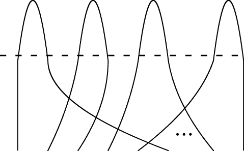
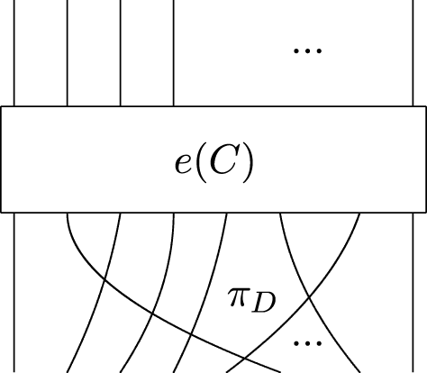
Proposition 4.8 is a restatement of Lemma 4.7. In terms of diagrams, the diagram  $D$ depicted in Figure 4 is taken to the element of
 ${\mathcal{B}}_{2d}^{2d}$ depicted in Figure 5.
The element  $\unicode[STIX]{x1D712}(D)$ of
 ${\mathcal{B}}_{2d}^{2d}$.

5 The SFT for $\text{OSp}(V)$

In this section, we continue with the notation above.  $V$ is a complex vector space with
 $\text{sdim }(V)=(m|2n)$. If
 $B(-,-)\in \text{Hom}(V^{2},\mathbb{C})$ is the given nondegenerate orthosymplectic form on
 $V$,
 $G=\text{OSp}(V)$ is its isometry group scheme, as explained in Section 2. The space
 $\left(\text{Hom}(V^{2d},\mathbb{C})\right)^{\text{OSp}(V)}$ of invariant multilinear maps has the universal scheme-theoretic meaning explained in Definition 1.1.
The FFT for  $\text{OSp}(V)$ asserts that the map
 $\unicode[STIX]{x1D705}$ in (4.8) (see Proposition 4.8) is surjective. The SFT for
 $\text{OSp}(V)$ describes the kernel of
 $\unicode[STIX]{x1D705}$.
5.1 The main theorem
The following theorem is the main result of this paper.
Theorem 5.1. Let  $\unicode[STIX]{x1D705}$ be the map in the commutative diagram (4.8). Then
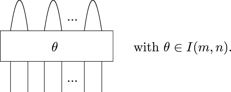
 $$\begin{eqnarray}\text{Ker}(\unicode[STIX]{x1D705})=D_{0}\circ I(m,n),\end{eqnarray}$$
where  $I(m,n)$ is the ideal of
 $\mathbb{C}\text{Sym}_{2d}$ which is the sum of the two-sided ideals corresponding to partitions which contain an
 $(m+1)\times (2n+1)$ rectangle and
 $D_{0}$ is the diagram in
 ${\mathcal{B}}_{2d}^{0}$ depicted in Figure 3.
Proof. Since the map  $h$ in (4.8) is injective, it follows that
 $\text{Ker}(\unicode[STIX]{x1D705})=\text{Ker}(\unicode[STIX]{x1D6FF}\circ \unicode[STIX]{x1D712})$. Hence,
 $b\in {\mathcal{B}}_{2d}^{0}$ lies in
 $\text{Ker}(\unicode[STIX]{x1D705})$ if and only if
 $\unicode[STIX]{x1D712}(b)\in \text{Ker}(\unicode[STIX]{x1D6FF})$, and by Corollary 2.5,
 $\text{Ker}(\unicode[STIX]{x1D6FF})={\mathcal{I}}_{2d}+I(m,n)$, where
 ${\mathcal{I}}_{2d}$ is the ideal generated by the nonmonic diagrams in
 ${\mathcal{B}}_{2d}^{2d}$. Moreover,
 $\unicode[STIX]{x1D6FF}$ factors through
 ${\mathcal{B}}_{2d}^{2d}/{\mathcal{I}}_{2d}\simeq \mathbb{C}\text{Sym}_{2d}$, and the kernel of the restriction of
 $\unicode[STIX]{x1D6FF}$ to
 $\mathbb{C}\text{Sym}_{2d}$ is
 $I(m,n)$.
But we claim that  $\unicode[STIX]{x1D712}^{-1}(I(m,n))=D_{0}\circ I(m,n)$, for if
 $x\in I(m,n)$, then by Proposition 4.8,
 $\unicode[STIX]{x1D712}(D_{0}\circ x)=e(C)x\in I(m,n)$, while conversely if
 $D_{0}\circ x\in \unicode[STIX]{x1D712}^{-1}(I(m,n))$ for some
 $x\in \mathbb{C}\text{Sym}_{2d}$, then
 $\unicode[STIX]{x1D712}(D_{0}\circ x)=e(C)x\in I(m,n)$. But then
 $D_{0}\circ x=D_{0}\circ e(C)x\in D_{0}\circ I(m,n)$, proving the assertion. The theorem follows.◻
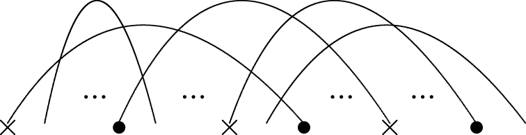
A typical element of the kernel of  $\unicode[STIX]{x1D705}$ is shown in Figure 6.
Elements of  $\text{Ker}(\unicode[STIX]{x1D705})$.

The following statement concerns the range of values of  $d$ for which
 $\text{Ker}(\unicode[STIX]{x1D705})\neq 0$.
Corollary 5.2. With notation as in Theorem 5.1, the kernel of  $\unicode[STIX]{x1D705}$ is zero if
 $2d<(m+1)(2n+1)$. Further,
 $\text{Ker}(\unicode[STIX]{x1D705})\neq 0$ for
 $d\geqslant (m+1)(2n+1)$.
Proof. The first assertion is immediate from Theorem 5.1. The second follows from the fact that
 $$\begin{eqnarray}I(m,n)=\mathbb{U}^{(m+1)(2n+1)}(D\circ (I(m,n)\otimes 1^{\otimes (m+1)(2n+1)})),\end{eqnarray}$$
where  $D:2(m+1)(2n+1)\rightarrow 0$ is the diagram with arcs
 $(i,2(m+1)(2n+1)-i+1)$,
 $i=1,\ldots ,(m+1)(2n+1)$ and
 $\mathbb{U}$ is the map described in the first paragraph of Section 5.2. The argument of
 $\mathbb{U}^{(m+1)(2n+1)}$ on the right side is therefore a nonzero element of
 $\text{Ker}(\unicode[STIX]{x1D705})$.◻
Note that as the discussion of the classical orthogonal and symplectic cases below shows, Corollary 5.2 is not optimal. Here is a nonclassical example.
Example 5.3. We take  $m=1=n$; thus, we are in the case of
 $\text{OSp}(1|2)$. In this case, the smallest value of
 $d$ for which
 $\text{Ker}(\unicode[STIX]{x1D705})$ could be nonzero is
 $d=3$ (
 $2d=(m+1)(2n+1)=2\times 3=6$). However, a straightforward calculation shows that in this case (i.e.,
 $d=3$), we have
 $D_{0}I(1,2)=0$ in
 $B_{6}^{0}$. Thus, here
 $\text{Ker}(\unicode[STIX]{x1D705})=0$ when
 $2d=(m+1)(2n+1)$. In fact, in this case, one sees that
 $\text{Ker}(\unicode[STIX]{x1D705})=0$ if and only if
 $d\leqslant 3$. For this, one must verify that
 $\text{Ker}(\unicode[STIX]{x1D705})\neq 0$ when
 $d=4$, that is, that
 $D_{0}I(1,2)\neq 0$ in
 $B_{8}^{0}$.
Remark 5.4. The available evidence seems to point to the statement that the smallest value of  $d$ for which
 $\text{Ker}(\unicode[STIX]{x1D705})\neq 0$ is
 $d=(m+1)(n+1)$ (i.e.,
 $2d=(m+1)(2n+1)+m+1$). This result has now been proved by Zhang in [Reference Zhang29, Theorem 5.11].
Note also that in [Reference Ehrig and Stroppel7], it is proved that  $\unicode[STIX]{x1D705}$ is injective for some small values of
 $d$.
5.2 Interpretation in the first formulation
Theorem 5.1 provides the SFT for  $\text{OSp}(V)$ in its second formulation; that is, it describes the linear structure of
 $\text{Hom}_{\mathbb{C}}(V^{\otimes 2d},\mathbb{C})^{\text{OSp}(V)}$. It may be useful to point out that it may be reinterpreted in terms of the Brauer algebra action
 $\unicode[STIX]{x1D702}_{r}:{\mathcal{B}}_{r}(m-2n)\longrightarrow \text{End}_{\text{OSp}(V)}(V^{\otimes r})$ (see [Reference Lehrer and Zhang19, Corollary 5.7]). For this, we note that in the Brauer category [Reference Lehrer and Zhang19], for nonnegative integers
 $p,q$ with
 $p>0$, there is an isomorphism
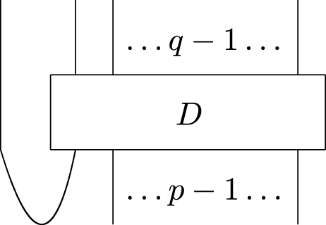
 $\mathbb{U}:{\mathcal{B}}_{p}^{q}\overset{{\sim}}{\longrightarrow }{\mathcal{B}}_{p-1}^{q+1}$. It is denoted by
 $\mathbb{U}_{p-1}^{1}$ in [Reference Lehrer and Zhang18, Corollary 2.8] and is depicted in Figure 7.
 $\mathbb{U}(D)$ for
 $D\in {\mathcal{B}}_{p}^{q}$.

One therefore has an isomorphism  $\mathbb{U}^{d}:{\mathcal{B}}_{2d}^{0}\longrightarrow {\mathcal{B}}_{d}^{d}$, and this leads to the following extension of the diagram (4.2).

The top map  $\unicode[STIX]{x1D702}:{\mathcal{B}}_{d}(m-2n)\rightarrow \text{End}_{\text{OSp}(V)}(V^{\otimes d})$ is precisely the map discussed in the paper [Reference Lehrer and Zhang18]. Theorem 5.1 has the following evident consequence.
Corollary 5.5. The kernel of the surjective algebra homomorphism  $\unicode[STIX]{x1D702}:{\mathcal{B}}_{d}(m-2n):={\mathcal{B}}_{d}^{d}\rightarrow \text{End}_{G}(V^{\otimes d})$ is
 $\mathbb{U}^{d}(D_{0}I(m,n))$.
Remark 5.6. In [Reference Lehrer and Zhang17] and [Reference Lehrer and Zhang18], we showed that in the classical cases when  $m=0$ or when
 $n=0$, the kernel is actually generated by a single idempotent in the associative algebra
 ${\mathcal{B}}_{d}(m-2n)$, but we do not have a similar result in the general case (cf. [Reference Zhang29]).
6 Application to the classical groups
In this final section, we shall show how our main theorem provides a new proof of the SFT in the classical cases of the orthogonal and symplectic groups over  $\mathbb{C}$ (see, e.g., [Reference Goodman and Wallach9, Reference Procesi21]). We therefore take
 $V$ as above and apply Theorem 5.1 in those respective cases.
6.1 The orthogonal case: $G=O(m,\mathbb{C})$

Here, we take  $V=V_{\bar{0}}$ to be purely even and the form
 $B(-,-)$ to be symmetric. To apply our result, observe that the ideal
 $I(m,n)=I(m,0)$ of
 $\mathbb{C}\text{Sym}_{2d}$ is spanned (over
 $\mathbb{C}$) by elements of the form
 $\unicode[STIX]{x1D70B}\unicode[STIX]{x1D6FC}^{-}(m+1)\unicode[STIX]{x1D70B}^{\prime }$, where
 $\unicode[STIX]{x1D70B},\unicode[STIX]{x1D70B}^{\prime }\in \text{Sym}_{2d}$ and for
 $\ell$ such that
 $1\leqslant \ell \leqslant 2d$,
 $\unicode[STIX]{x1D6FC}^{-}(\ell )=\sum _{\unicode[STIX]{x1D70E}\in \text{Sym}_{\ell }}\unicode[STIX]{x1D700}(\unicode[STIX]{x1D70E})\unicode[STIX]{x1D70E}$, where
 $\unicode[STIX]{x1D700}$ is the alternating character of
 $\text{Sym}_{2d}$ and
 $\text{Sym}_{\ell }\subseteq \text{Sym}_{2d}$ is the subgroup which permutes the first
 $\ell$ symbols.
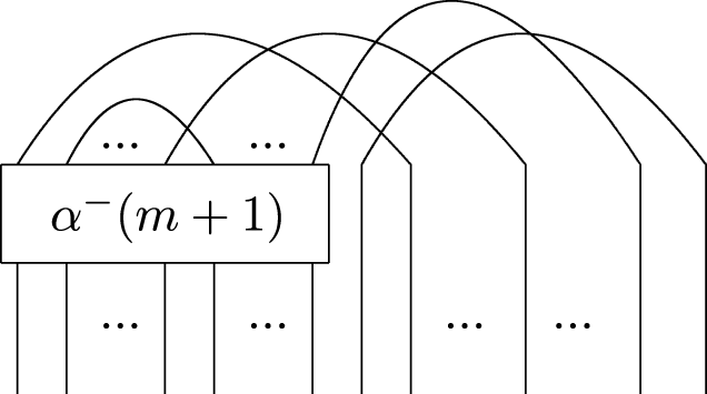
Theorem 5.1 asserts that  $\text{Ker}\left(\unicode[STIX]{x1D705}:{\mathcal{B}}_{2d}^{0}(\mathbb{C})\longrightarrow \text{Hom}_{\mathbb{C}}(V^{\otimes 2d},\mathbb{C})^{\text{OSp}(V)}\right)$ is spanned by the elements
 $D_{0}\unicode[STIX]{x1D70B}\unicode[STIX]{x1D6FC}^{-}(m+1)\unicode[STIX]{x1D70B}^{\prime }$. The next lemma shows that if
 $d$ is small, the kernel is zero.
Lemma 6.1. If  $d\leqslant m$, then each element
 $D_{0}\unicode[STIX]{x1D70B}\unicode[STIX]{x1D6FC}^{-}(m+1)\unicode[STIX]{x1D70B}^{\prime }$ of
 ${\mathcal{B}}_{2d}^{0}$ is zero.
Proof. Let  $\unicode[STIX]{x1D70B}\in \text{Sym}_{2d}$ and consider the diagram
 $D=D_{0}\unicode[STIX]{x1D70B}$. If
 $d\leqslant m$, then
 $d<m+1$, and it follows that at least one arc of
 $D$ has both ends in
 $\{1,2,\ldots ,m+1\}$ (if each arc with an end in
 $\{1,2,\ldots ,m+1\}$ had an end outside
 $\{1,2,\ldots ,m+1\}$, we would have
 $2d\geqslant 2(m+1)$). Suppose this arc is from
 $i$ to
 $j$, where
 $1\leqslant i<j\leqslant m+1$, and write
 $(ij)$ for the transposition in
 $\text{Sym}_{2d}$ which interchanges
 $i$ and
 $j$.
Then by the rules for multiplying Brauer diagrams, we have  $D(ij)=D$, whence
 $D_{0}\unicode[STIX]{x1D70B}(ij)\unicode[STIX]{x1D6FC}^{-}(m+1)=D_{0}\unicode[STIX]{x1D70B}\unicode[STIX]{x1D6FC}^{-}(m+1)$.
But by the alternating property of  $\unicode[STIX]{x1D6FC}^{-}(m+1)$, we have
 $(ij)\unicode[STIX]{x1D6FC}^{-}(m+1)=-\unicode[STIX]{x1D6FC}^{-}(m+1)$, whence
 $D_{0}\unicode[STIX]{x1D70B}(ij)\unicode[STIX]{x1D6FC}^{-}(m+1)=-D_{0}\unicode[STIX]{x1D70B}\unicode[STIX]{x1D6FC}^{-}(m+1)$. The lemma follows.◻
Figure 8 depicts an example of a linear combination of diagrams which is zero by Lemma 6.1.
Corollary 6.2. If  $d\leqslant m$, then
 $\text{Ker}(\unicode[STIX]{x1D705})=0$, and
 $\unicode[STIX]{x1D705}:{\mathcal{B}}_{2d}^{0}(\mathbb{C})\longrightarrow \text{Hom}_{\mathbb{C}}(V^{\otimes 2d},\mathbb{C})^{\text{O}(V)}$ is an isomorphism.
Our main theorem now has the following interpretation in the present case (cf. [Reference Lehrer and Zhang18, Theorem 3.4]). Recall that diagrams  $D\in {\mathcal{B}}_{2d}^{0}$ are in canonical bijection with partitions of
 $\{1,\ldots ,2d\}$ into pairs.
Theorem 6.3. Let  $V=V_{\bar{0}}=\mathbb{C}^{m}$ and
 $G=O(m,\mathbb{C})$. If
 $d\leqslant m$, then
 $\text{Ker}(\unicode[STIX]{x1D705})=0$. Assume that
 $d\geqslant m+1$.
Define a set of linear relations among the  $\unicode[STIX]{x1D705}_{D}$ as follows. Let
 $S,S^{\prime }$ be two disjoint subsets of
 $\{1,\ldots ,2d\}$ as depicted in Figure 9 such that
 $|S|=|S^{\prime }|=m+1$, and for
 $\unicode[STIX]{x1D70E}\in \text{Sym}(\{S\})$, let
 $D(\unicode[STIX]{x1D70B},\unicode[STIX]{x1D70B}^{\prime };\unicode[STIX]{x1D70E})$ be the diagram in
 ${\mathcal{B}}_{2d}^{0}$ which pairs
 $\unicode[STIX]{x1D70E}(s_{i})$ with
 $s_{i}^{\prime }$, where the
 $s_{i}\in S,s_{i}^{\prime }\in S^{\prime }$ are written in increasing order, and the points in
 $\{1,\ldots ,2d\}\setminus (S\cup S^{\prime })$ are paired as they are in each diagram occurring in
 $D_{0}\unicode[STIX]{x1D70B}\unicode[STIX]{x1D6FC}^{-}(m+1)\unicode[STIX]{x1D70B}^{\prime }$.
Zero element in  ${\mathcal{B}}_{2d}^{0}$.

Then for each  $\unicode[STIX]{x1D70B},\unicode[STIX]{x1D70B}^{\prime }\in \text{Sym}_{2d}$,
 $$\begin{eqnarray}\displaystyle \mathop{\sum }_{\unicode[STIX]{x1D70E}\in \text{Sym}_{m+1}}\unicode[STIX]{x1D700}(\unicode[STIX]{x1D70E})\unicode[STIX]{x1D705}_{D(\unicode[STIX]{x1D70B},\unicode[STIX]{x1D70B}^{\prime },\unicode[STIX]{x1D70E})}=0, & & \displaystyle\end{eqnarray}$$
and all relations among the  $\unicode[STIX]{x1D705}_{D}$ are linear consequences of these relations.
Proof. The first statement is Corollary 6.2.
By Theorem 5.1, all relations among the  $\unicode[STIX]{x1D705}_{D}$ are consequences of the relations
 $\unicode[STIX]{x1D705}(D_{0}\unicode[STIX]{x1D70B}\unicode[STIX]{x1D6FC}^{-}(m+1)\unicode[STIX]{x1D70B}^{\prime })=0$, for
 $\unicode[STIX]{x1D70B},\unicode[STIX]{x1D70B}^{\prime }\in \text{Sym}_{2d}$.
Now the argument of the proof of Lemma 6.1 shows that if two of the points in the set  $S:=\{\unicode[STIX]{x1D70B}^{-1}(1),\unicode[STIX]{x1D70B}^{-1}(2),\ldots ,\unicode[STIX]{x1D70B}^{-1}(m+1)\}$ are paired by
 $D_{0}$ then
 $D_{0}\unicode[STIX]{x1D70B}\unicode[STIX]{x1D6FC}^{-}(m+1)\unicode[STIX]{x1D70B}^{\prime }=0$ in
 ${\mathcal{B}}_{2d}^{0}$, and so to obtain a nonzero element of the kernel, we may assume that no two points in
 $S$ are paired by
 $D_{0}$ and, hence, that the set
 $S^{\prime }$ of points which are paired by
 $D_{0}$ with a point of
 $S$ is disjoint from
 $S$.
In this case, the relation  $\unicode[STIX]{x1D705}(D_{0}\unicode[STIX]{x1D70B}\unicode[STIX]{x1D6FC}^{-}(m+1)\unicode[STIX]{x1D70B}^{\prime })=0$ is easily seen to translate into (6.1), and the result is now clear.◻
The set  $S$ consists of
 $\bullet$’s and
 $S^{\prime }$ of
 $\times$’s.

6.2 The symplectic case
In this case, we take  $V=V_{\bar{1}}$. The form
 $B(-,-)$ is then skew, and
 $G=\text{Sp}(2n,\mathbb{C})$. The ideal
 $I(m,n)=I(0,n)$ is, in this case, spanned (over
 $\mathbb{C}$) by elements of the form
 $\unicode[STIX]{x1D70B}\unicode[STIX]{x1D6FC}^{+}(2n+1)\unicode[STIX]{x1D70B}^{\prime }$, where
 $\unicode[STIX]{x1D70B},\unicode[STIX]{x1D70B}^{\prime }\in \text{Sym}_{2d}$ and for each integer
 $\ell$ with
 $1\leqslant \ell \leqslant 2d$,
 $\unicode[STIX]{x1D6FC}^{+}(\ell )=\sum _{\unicode[STIX]{x1D70E}\in \text{Sym}_{\ell }}\unicode[STIX]{x1D70E}$, where as above,
 $\text{Sym}_{\ell }\subseteq \text{Sym}_{2d}$ is the subgroup which permutes the first
 $\ell$ symbols.
In this case, the analogue of Lemma 6.1 is the trivial observation that there are no nonzero elements of the kernel unless  $2d\geqslant 2n+1$, that is,
 $d\geqslant n+1$.
Taking into account the fact that for a symplectic form  $(v,v)=0$ for all
 $v\in V$, we obtain the following form of the main theorem for the symplectic case.
Theorem 6.4. Let  $V=V_{\bar{1}}=\mathbb{C}^{2n}$, and
 $G=\text{Sp}(2n,\mathbb{C})$. If
 $d\leqslant n$, then
 $\text{Ker}(\unicode[STIX]{x1D705})=0$. Assume that
 $d\geqslant n+1$.
Define a set of linear relations among the  $\unicode[STIX]{x1D705}_{D}$ as follows. Let
 $S$ be a subset of
 $\{1,\ldots ,2d\}$ such that
 $|S|=2n+1$. For any diagram
 $D\in {\mathcal{B}}_{2d}^{0}$ and
 $\unicode[STIX]{x1D70E}\in \text{Sym}(\{S\})$, let
 $D(S,\unicode[STIX]{x1D70E})$ be the diagram
 $D(S,\unicode[STIX]{x1D70E})=D\unicode[STIX]{x1D70E}$, where
 $\unicode[STIX]{x1D70E}$ is regarded as an element of
 $\text{Sym}_{2d}\subset {\mathcal{B}}_{2d}^{2d}$ which fixes the points outside
 $S$.
Then
 $$\begin{eqnarray}\displaystyle \mathop{\sum }_{\unicode[STIX]{x1D70E}\in \text{Sym}(\{S\})}\unicode[STIX]{x1D705}_{D(S,\unicode[STIX]{x1D70E})}=0, & & \displaystyle\end{eqnarray}$$
and all relations among the  $\unicode[STIX]{x1D705}_{D}$ are linear consequences of these relations.
This is clear from Theorem 5.1.
Acknowledgments
The authors are grateful to the referee, whose detailed suggestions have significantly enhanced this paper.
Appendix A. Superpolarization
Proposition A.1. Let  $M_{\mathbb{C}}$ be a
 $\mathbb{Z}/2\mathbb{Z}$-graded complex vector space with
 $\text{sdim }(M_{\mathbb{C}})=(k|\ell )$, let
 $A$ be a supercommutative super
 $\mathbb{C}$-algebra, and let
 $M=M_{\mathbb{C}}\otimes _{\mathbb{C}}A$,
 $\mathbb{Z}/2\mathbb{Z}$-graded in the usual way. Let
 $B\subseteq M_{\bar{0}}$ be a subset satisfying the conditions
(i)
$AB=M$; that is, $B$ generates $M$ as $A$-module.(ii) For any two distinct elements
$b,c\in B$, there are infinitely many complex numbers $\unicode[STIX]{x1D706}$ such that $b+\unicode[STIX]{x1D706}c\in B$.


Let  $T^{r}(M)=M\otimes _{A}M\otimes _{A}\cdots \otimes _{A}M$ (
 $r$ factors), and let
 $S^{r}(M)$ be the supersymmetric part of
 $T^{r}(M)$ (cf. [Reference Lehrer and Zhang19, Section 3]).
Then for each integer  $r\geqslant 0$, the space
 $\left(S^{r}(M)\right)_{\bar{0}}$ is the
 $A_{\bar{0}}$-span of the elements
 $\{b\otimes b\otimes \cdots \otimes b\mid b\in B\}$.
Proof. This will be by induction on  $r$, the case
 $r=1$ being trivial, since by the condition (i),
 $A_{\bar{0}}B=M_{\bar{0}}$ so that
 $M_{\bar{0}}$ is the
 $A_{\bar{0}}$-span of
 $B$ (and
 $M_{\bar{1}}$ is the
 $A_{\bar{1}}$-span of
 $B$).
Now it follows from [Reference Lehrer and Zhang19, Lemma 3.7] that  $S^{r}(M)=\unicode[STIX]{x1D6FC}^{+}(r)T^{r}(M)$, where
 $\unicode[STIX]{x1D6FC}^{+}(r)=\sum _{\unicode[STIX]{x1D70E}\in \text{Sym}_{r}}\unicode[STIX]{x1D70E}$, with
 $\text{Sym}_{r}$ acting on
 $T^{r}(M)$ in the usual way through
 $\unicode[STIX]{x1D71B}_{r}$ (see (2.2)). Denote by
 $\unicode[STIX]{x1D6F4}(r)$ the
 $A_{\bar{0}}$-span of
 $\{b\otimes b\otimes \cdots \otimes b\mid b\in B\}$. Then by the last remark, it suffices to show that for any element
 $m_{1}\otimes m_{2}\otimes \cdots \otimes m_{r}\in T^{r}(M)_{\bar{0}}$, we have
 $$\begin{eqnarray}\displaystyle \unicode[STIX]{x1D6FC}^{+}(r)(m_{1}\otimes m_{2}\otimes \cdots \otimes m_{r})\in \unicode[STIX]{x1D6F4}(r). & & \displaystyle\end{eqnarray}$$
We shall prove (A1) by induction on  $r$. Assume (A1) for a smaller number of factors; we consider separately two cases.
Case 1: at least one of the factors  $m_{i}$ lies in
 $M_{\bar{0}}$. In this case, since for any element
 $\unicode[STIX]{x1D70E}\in \text{Sym}_{r}$ we have
 $\unicode[STIX]{x1D6FC}^{+}(r)\unicode[STIX]{x1D70E}=\unicode[STIX]{x1D6FC}^{+}(r)$, we may clearly assume that
 $m_{r}\in M_{\bar{0}}$. Then
 $m_{1}\otimes m_{2}\otimes \cdots \otimes m_{r-1}\in T^{r-1}(M)_{\bar{0}}$, and by induction, we have
 $\unicode[STIX]{x1D6FC}^{+}(r-1)(m_{1}\otimes m_{2}\otimes \cdots \otimes m_{r-1})\in \unicode[STIX]{x1D6F4}(r-1)$.
But from the coset decomposition of  $\text{Sym}_{r}$ with respect to
 $\text{Sym}_{r-1}$, we have
 $$\begin{eqnarray}\unicode[STIX]{x1D6FC}^{+}(r)=\left(1+\mathop{\sum }_{i=1}^{r-1}(i,r)\right)\unicode[STIX]{x1D6FC}^{+}(r-1),\end{eqnarray}$$
where  $(i,j)$ denotes the transposition of
 $i$ and
 $j$ in
 $\text{Sym}_{r}$ and
 $\text{Sym}_{r-1}$ is the subgroup of
 $\text{Sym}_{r}$ which permutes
 $\{1,\ldots ,r-1\}$. The last two observations imply that
 $\unicode[STIX]{x1D6FC}^{+}(r)(m_{1}\otimes m_{2}\otimes \cdots \otimes m_{r})$ is a
 $A_{\bar{0}}$-linear combination of elements of the form
 $$\begin{eqnarray}\displaystyle \left(1+\mathop{\sum }_{i=1}^{r-1}(i,r)\right)(b\otimes b\otimes \cdots \otimes b\otimes c), & & \displaystyle\end{eqnarray}$$
where  $b,c\in B$.
Now denote by  $s_{i,j}(b,c)$ the sum of all tensors of the form
 $\cdots \otimes b\otimes \cdots \otimes c\otimes \cdots \in T^{r}(M)$, where all factors are either
 $b$ or
 $c$, and there are
 $i$ factors equal to
 $b$ and
 $j$ factors equal to
 $c$. Then the element in (A2) is
 $s_{1,r-1}(b,c)$, and it will suffice to show that if
 $b,c\in B$, then
 $s_{i,j}(b,c)\in \unicode[STIX]{x1D6F4}(r)$ for all
 $i,j$ such that
 $i+j=r$. To see this last point, suppose
 $\unicode[STIX]{x1D706}\in \mathbb{C}$ is such that
 $b+\unicode[STIX]{x1D706}c\in B$. Then
 $\unicode[STIX]{x1D6F4}(r)\ni (b+\unicode[STIX]{x1D706}c)\otimes (b+\unicode[STIX]{x1D706}c)\otimes \cdots \otimes (b+\unicode[STIX]{x1D706}c)=\sum _{j=0}^{r}\unicode[STIX]{x1D706}^{j}s_{i,j}(b,c)$. By taking
 $r+1$ distinct values
 $\unicode[STIX]{x1D706}$ for which this relation holds, we obtain, by the invertibility of the van der Monde matrix, an equation for each element
 $s_{i,j}(b,c)$ as a
 $\mathbb{C}$-linear combination of the elements
 $(b+\unicode[STIX]{x1D706}c)\otimes (b+\unicode[STIX]{x1D706}c)\otimes \cdots \otimes (b+\unicode[STIX]{x1D706}c)\in \unicode[STIX]{x1D6F4}(r)$. Thus,
 $s_{r-1,1}(b,c)\in \unicode[STIX]{x1D6F4}(r)$, and the proof in Case 1 is complete.
Case 2: each factor  $m_{i}\in M_{\bar{1}}$. In this case, we must have
 $r$ even. Since
 $\unicode[STIX]{x1D6FC}^{+}(r)$ is linear in each variable
 $m_{i}$ and since
 $M_{\bar{1}}=A_{\bar{1}}B$, we may assume that for
 $i=1,2,\ldots ,r$, we have
 $m_{i}=\unicode[STIX]{x1D706}_{i}b_{i}$, where
 $\unicode[STIX]{x1D706}_{i}\in A_{\bar{1}}$ and
 $b_{i}\in B$. Then
 $$\begin{eqnarray}\displaystyle \unicode[STIX]{x1D6FC}^{+}(r)(\unicode[STIX]{x1D706}_{1}b_{1}\otimes \cdots \unicode[STIX]{x1D706}_{r}b_{r}) & = & \displaystyle \mathop{\sum }_{\unicode[STIX]{x1D70E}\in \text{Sym}_{r}}\unicode[STIX]{x1D70E}(\unicode[STIX]{x1D706}_{1}b_{1}\otimes \cdots \unicode[STIX]{x1D706}_{r}b_{r})\nonumber\\ \displaystyle & = & \displaystyle \mathop{\sum }_{\unicode[STIX]{x1D70E}\in \text{Sym}_{r}}\unicode[STIX]{x1D700}(\unicode[STIX]{x1D70E})\unicode[STIX]{x1D706}_{\unicode[STIX]{x1D70E}(1)}\unicode[STIX]{x1D706}_{\unicode[STIX]{x1D70E}(2)}\cdots \unicode[STIX]{x1D706}_{\unicode[STIX]{x1D70E}(r)}b_{\unicode[STIX]{x1D70E}(1)}\otimes \cdots \otimes b_{\unicode[STIX]{x1D70E}(r)}\nonumber\\ \displaystyle & = & \displaystyle \mathop{\sum }_{\unicode[STIX]{x1D70E}\in \text{Sym}_{r}}\unicode[STIX]{x1D700}(\unicode[STIX]{x1D70E})^{2}\unicode[STIX]{x1D706}_{1}\unicode[STIX]{x1D706}_{2}\cdots \unicode[STIX]{x1D706}_{r}b_{\unicode[STIX]{x1D70E}(1)}\otimes \cdots \otimes b_{\unicode[STIX]{x1D70E}(r)}\nonumber\\ \displaystyle & = & \displaystyle \unicode[STIX]{x1D706}_{1}\unicode[STIX]{x1D706}_{2}\cdots \unicode[STIX]{x1D706}_{r}\unicode[STIX]{x1D6FC}^{+}(r)(b_{1}\otimes \cdots \otimes b_{r}),\nonumber\end{eqnarray}$$
where  $\unicode[STIX]{x1D700}$ is the alternating character of
 $\text{Sym}_{r}$. But since
 $r$ is even,
 $\unicode[STIX]{x1D706}_{1}\cdots \unicode[STIX]{x1D706}_{r}\in A_{\bar{0}}$; finally, observe that by Case 1,
 $\unicode[STIX]{x1D6FC}^{+}(r)(b_{1}\otimes \cdots \otimes b_{r})\in \unicode[STIX]{x1D6F4}(r)$, and the proof is complete.◻
Corollary A.2. Let  $F\in S^{d}(M^{\ast })$ be a function of degree
 $d$ on the affine superspace
 $M$. Then there exists a function
 $\widetilde{F}\in {\mathcal{H}}om(M^{d},\mathbb{G}_{a})$ such that
 $F(m)=\widetilde{F}(m,\ldots ,m)$.
Proof. Take  $B=M(A)_{\bar{0}}$ in Proposition A.1.◻