1. Introduction
Shear coaxial jets, in which a circular jet flows inside an annular jet, are canonical flows found in many applications, for example liquid rocket engines. Despite the simplicity of the geometry, the flows exhibit very complex dynamical behaviour and non-trivial interactions with the dynamics of their surroundings (Hopfinger Reference Hopfinger and Frisch1998; Hong et al. Reference Hong, Fusetti, De Rosa and Oschwald2006), one important interaction being with coherent acoustic waves. They are important, for instance, in combustion chambers experiencing combustion-induced acoustic instabilities (Miesse Reference Miesse1955; Wicker & Eaton Reference Wicker and Eaton1994; Villermaux, Rehab & Hopfinger Reference Villermaux, Rehab and Hopfinger1998; Davis & Chehroudi Reference Davis and Chehroudi2006, Reference Davis and Chehroudi2007; Leyva et al. Reference Leyva, Rodriguez, Chehroudi and Talley2007; Teshome Reference Teshome2012). If the acoustic–jet interaction is such that pressure fluctuations become phase coherent with heat-release fluctuations, the acoustics can amplify temperature gradients and cause damage to the combusting system. Thus, it is important to gain an understanding of how different geometries and flow conditions affect the nature of the coupling between acoustic waves and coaxial jets.
Teshome (Reference Teshome2012) studied the simplified case of acoustic waves interacting with non-reacting shear coaxial jets. He performed modal decomposition of high-frequency high-resolution shadowgraph imaging. Because applications usually have complex geometries, it is inefficient to perform such decompositions using predetermined basis functions. It is more appropriate to use techniques such as proper orthogonal decomposition (POD) (Lumley Reference Lumley1967; Sirovich Reference Sirovich1987a ,Reference Sirovich b ,Reference Sirovich c ; Berkooz et al. Reference Berkooz, Holmes and Lumley1993), in which the basis functions are derived as part of the analysis. This approach was used by Teshome (Reference Teshome2012); however, only the nature of the primary POD modes in the flows was reported.
In the present study, we extend the analysis of Teshome’s data using an alternative decomposition based on Koopman eigenfunctions (Mezic & Banaszuk Reference Mezic and Banaszuk2004; Rowley et al. Reference Rowley, Mezic, Bagheri, Schlatter and Henningson2009; Mezic Reference Mezic, Davis and Moin2013; Motheau et al. Reference Motheau, Mery, Nicoud and Poinsot2013). Koopman decomposition (Mezic & Banaszuk Reference Mezic and Banaszuk2004; Rowley et al. Reference Rowley, Mezic, Bagheri, Schlatter and Henningson2009; Budišić, Mohr & Mezić Reference Budišić, Mohr and Mezić2012; Mezic Reference Mezic, Davis and Moin2013) is a natural approach to search for collective oscillatory behaviour and is based on the Koopman operator theory (Rowley et al. Reference Rowley, Mezic, Bagheri, Schlatter and Henningson2009; Schmid Reference Schmid2010; Mezic Reference Mezic, Davis and Moin2013), which generalizes eigendecomposition to nonlinear systems. Koopman modes are a generalization of normal modes (Mezic Reference Mezic, Davis and Moin2013), and each mode represents a global collective motion within a flow. Importantly, spectral properties of the flow will be contained in the spectrum of the Koopman operator (Rowley et al. Reference Rowley, Mezic, Bagheri, Schlatter and Henningson2009; Mezic Reference Mezic, Davis and Moin2013). A fast algorithm proposed by Schmid (Reference Schmid2010) and referred to as dynamic-mode decomposition (DMD) can be used for computing approximately (a subset of) the Koopman spectrum from the time series of snapshots of the flow.
Each Koopman mode is associated with a complex eigenvalue whose real and imaginary parts represent the growth rate and frequency of the mode respectively. These eigenvalues can be used to address a critical issue in the analysis of nonlinear flows, namely how to differentiate robust features of the flow from noise and other non-robust characteristics. As we contend (Roy et al. Reference Roy, Hua, Barnhill, Gunaratne and Gord2015), comparison of Koopman spectra from nominally identical experiments can be the basis of this differentiation. The starting point is a search for reproducible Koopman modes, i.e. those that persist in different experiments. The differentiation is based on the following conjecture: robust characteristics of the flow can be associated with reproducible Koopman modes. Only robust features are expected to be useful in applications such as flow control.
Injector flows are introduced in § 2, and Koopman mode analysis and the relevant computational techniques are summarized in § 3. The results of the modal decomposition of injector flows for a series of control parameters are presented in § 4. Section 5 contains a discussion of the implications of our results.
2. Injector flows
The experiments in the non-reactive shear coaxial study were conducted in the Cryogenic Supercritical Flow Facility (EC-4) at the Air Force Research Laboratory located at Edwards Air Force Base, CA. The fluid used in these studies was
 $\text{N}_{2}$
at ambient conditions tapped from a high-pressure supply line. Liquid
 $\text{N}_{2}$
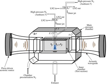
was used for temperature control (Teshome Reference Teshome2012). The pressure within the chamber could be as high as 36 atm. A schematic of the experimental facility is shown in figure 1.
Injector flows were observed with shadowgraph imaging using diffuse backscattering and recorded using Phantom v7.1 and v710 high-speed cameras (Teshome Reference Teshome2012). High-density regions appeared dark. The flow was analysed through a modal decomposition implemented through Koopman mode analysis, described below.
Schematic of the chamber and peripheral lines. The light long arrows point to constituents of the device and the heavy short arrows give the flow directions of gasses. Courtesy of Teshome (Reference Teshome2012).

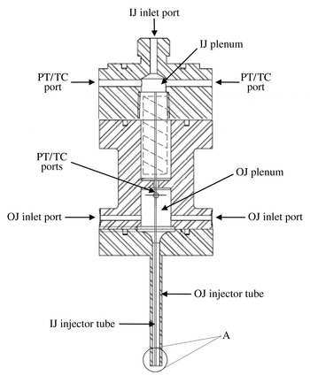
The shear coaxial injector consisted of concentric straight tubes, where the inner jet flowed through the centre tube and the outer jet flowed through the annulus. A schematic of a sectional view of the entire injector assembly is shown in figure 2.
Schematic of the shear coaxial injector assembly (for expanded view of A, see figure 3) (from Teshome Reference Teshome2012).

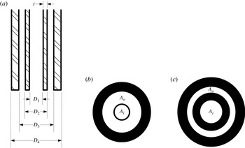
Schematic of the shear coaxial injector exit (from Teshome Reference Teshome2012): (a) expanded view of A in figure 2; (b) LAR-thin; (c) SAR-thick.

The inner jet was introduced through the top inlet hole of the assembly and entered a small plenum, which served as a settling chamber for the flow. The outer jet was introduced into a settling chamber through two ports located on the side of the assembly. Two parameters were varied for the two types of injectors constructed from 316 stainless steel: (1) the ratio of the inner-jet tube thickness to the diameter of the inner-jet tube and (2) the ratio of the outer-jet to inner-jet cross-sectional areas. Figure 3 is a schematic of the dimensions of the injector exit. The first injector with the large area ratio (LAR) and thin inner-tube post is labelled ‘LAR-thin’, while the second injector with the small area ratio (SAR) and thick post is labelled ‘SAR-thick’. The results reported here are for the LAR-thin configuration; flows in the other injector tube set-up are similar but contain significantly higher levels of noise. For the same reason, we focus on subcritical-chamber-pressure experiments. The dimensions of the injector cross-section for the LAR-thin configuration were
 $D_{1}=0.70$
mm,
 $D_{2}=0.89$
mm,
 $D_{3}=2.44$
mm and
 $D_{4}=3.94$
mm.
The physical parameters of the coaxial jet flow were based on the injector exit flow properties. They are characterized by
 $J$
, the outer-to-inner-jet momentum flux ratio,
 ${\it\rho}_{o}U_{o}^{2}/{\it\rho}_{i}U_{i}^{2}$
, where
 ${\it\rho}$
and
 $U$
are the density and velocity of the flow respectively. For ‘LAR-thin-subcritial’ experiments, the available values of
 $J$
are 0.1, 0.5, 2.1, 5.2, 11, 14 and 20.
The experimental set-up for injector flows in the absence of additional perturbations (referred to as baseline flows) was rotationally invariant about the axis of the flow. We also analysed flows that were subjected to transverse acoustic perturbations imposed using a waveguide attached to each side of a rectangular test section, as shown in figure 1. These perturbations break the rotational symmetry of the experimental configuration. Two types of acoustic driving were performed in the experiments: (1) those where the injector was placed at a pressure antinode (PAN) and (2) those where it was placed at a pressure node (PN). We focus on injector flows subjected to PAN driving; they contain lower levels of noise.
Each image was recorded on a grid of
 $192\times 302$
with a resolution of
 $22~{\rm\mu}\text{m}$
; thus the image dimensions are
 $4.2~\text{mm}\times 6.6~\text{mm}$
. The image capture began close to the initiation of the injector flow and transients could be observed through the Koopman mode analysis, as seen below. The transients were especially long for smaller values of
 $J$
.
3. Koopman modes and dynamic-mode decompositions
3.1. Modal decomposition
Proper orthogonal decomposition (Lumley Reference Lumley1967; Sirovich Reference Sirovich1987a ,Reference Sirovich b ,Reference Sirovich c ) has been used to analyse patterns within injector flows (Teshome Reference Teshome2012; Tirunagari et al. Reference Tirunagari, Hulkkonene, Vuorinen, Kaario and Larmi2012a ,Reference Tirunagari, Vuorinen, Kaario and Larmi b ). The analyses provide the structure of proper orthogonal modes and the relative contributions to the flow from each mode. Typically, modes with larger contributions are associated with the regular constituents of the underlying flow and those with lower contributions are assumed to be noise and other irregular facets of the flow. However, there has not been a verification of this flow differentiation. Previous DMDs of sprays (Tirunagari et al. Reference Tirunagari, Vuorinen, Kaario and Larmi2012b ) have also not addressed the issue. The analysis reported here is motivated by an approach introduced in Roy et al. (Reference Roy, Hua, Barnhill, Gunaratne and Gord2015) and outlined below which differentiates robust and non-robust constituents of a flow using Koopman mode analysis (Rowley et al. Reference Rowley, Mezic, Bagheri, Schlatter and Henningson2009; Schmid Reference Schmid2010; Mezic Reference Mezic, Davis and Moin2013). As we observe from figures 15 and 24 below, robust and non-robust constituents of injector flows cannot be differentiated using their contributions to the flow alone.
Koopman mode analysis of spatio-temporal fluid density fields is included for completeness and follows Lumley (Reference Lumley1967), Sirovich (Reference Sirovich1987a
,Reference Sirovich
b
,Reference Sirovich
c
), Rowley et al. (Reference Rowley, Mezic, Bagheri, Schlatter and Henningson2009), Schmid (Reference Schmid2010) and Mezic (Reference Mezic, Davis and Moin2013). Suppose that the state of a dynamical system is
 $\boldsymbol{z}$
and that its dynamics is given by
 $$\begin{eqnarray}\dot{\boldsymbol{z}}=\mathscr{F}(\boldsymbol{z}),\end{eqnarray}$$
with constraints and restrictions such as an appropriate set of boundary conditions. The dynamics evolves from the initial state
 $\boldsymbol{z}_{0}$
of the system to
 $\boldsymbol{z}_{t}\equiv \unicode[STIX]{x1D64E}^{t}(\boldsymbol{z}_{0})$
at time
 $t$
. In the case of fluid dynamics of injector flows,
 $\mathscr{F}$
consists of the Navier–Stokes equations with, perhaps, no-slip boundary conditions. Although this is the most compact representation of the flow, it is difficult to solve the system under realistic conditions, especially for high Reynolds numbers. On the other hand, high-quality empirical data are available on various secondary fields associated with the dynamical system, e.g. the density field of the injector flows. Let us represent one such (observable) secondary field (associated with
 $\boldsymbol{z}$
) by
 $u[\boldsymbol{z}](\boldsymbol{x})$
, where
 $\boldsymbol{x}$
represents the grid points on which the observations are made. As the state of the system evolves from
 $\boldsymbol{z}_{0}$
at time
 $t=0$
to
 $\boldsymbol{z}_{t}$
at time
 $t$
, the secondary field evolves from
 $u[\boldsymbol{z}_{0}](\boldsymbol{x})$
to
 $u[\boldsymbol{z}_{t}](\boldsymbol{x})$
. When the context is clear, one can simplify the notation by writing
 $u(\boldsymbol{x},t)$
for
 $u[\boldsymbol{z}_{t}](\boldsymbol{x})$
.
Koopman analysis (Mezic & Banaszuk Reference Mezic and Banaszuk2004; Rowley et al.
Reference Rowley, Mezic, Bagheri, Schlatter and Henningson2009; Budišić et al.
Reference Budišić, Mohr and Mezić2012; Mezic Reference Mezic, Davis and Moin2013) of the system is conducted on the ‘observable’
 $\boldsymbol{u}[\boldsymbol{z}](\boldsymbol{x},t)$
. An initial function
 $\boldsymbol{u}[\boldsymbol{z}_{0}](\boldsymbol{x},t=0)$
evolves to a function
 $\boldsymbol{u}[\boldsymbol{z}_{t}](\boldsymbol{x},t)$
at time
 $t$
. The transformation between the functions is given by the Koopman (or composition) operator, which is defined as
 $$\begin{eqnarray}U^{t}\boldsymbol{ : }\boldsymbol{u}[\boldsymbol{z}_{0}](\boldsymbol{x},t=0)\rightarrow \boldsymbol{u}[\boldsymbol{z}_{t}](\boldsymbol{x},t).\end{eqnarray}$$
It should be noted that even when
 $\unicode[STIX]{x1D64E}^{t}$
is finite-dimensional and nonlinear, the Koopman operator
 $U^{t}$
is infinite-dimensional and linear (Rowley et al.
Reference Rowley, Mezic, Bagheri, Schlatter and Henningson2009; Mezic Reference Mezic, Davis and Moin2013). Since both
 $\unicode[STIX]{x1D64E}^{t}$
and
 $U^{t}$
describe the same flow, one expects common features in the descriptions. For example, if the injector flow were uniform in time,
 $\boldsymbol{z}_{0}$
would be a fixed point of
 $\unicode[STIX]{x1D64E}^{t}$
and
 $\boldsymbol{u}[\boldsymbol{z}_{0}](\boldsymbol{x},t=0)$
would be a fixed point of
 $U^{t}$
. In periodic flows, the periodicity will be reflected in the spectra of
 $\boldsymbol{z}_{t}$
as well as in the spectra of
 $\boldsymbol{u}[\boldsymbol{z}_{t}](\boldsymbol{x},t)$
. In fact, it is known that spectral properties of
 $\unicode[STIX]{x1D64E}^{t}$
are contained in the eigenspectrum of
 $U^{t}$
. Eigenvalues of
 $U^{t}$
form the Koopman spectrum, and the corresponding eigenfunctions are referred to as Koopman eigenfunctions. Coefficients in the projection of
 $\boldsymbol{u}[\boldsymbol{z}_{t}](\boldsymbol{x},t)$
to the Koopman eigenfunctions form the Koopman modes of the state (Rowley et al.
Reference Rowley, Mezic, Bagheri, Schlatter and Henningson2009). As the system evolves under
 $\unicode[STIX]{x1D64E}^{t}$
, the
 $k$
th Koopman mode evolves as
 $\text{e}^{{\it\mu}_{k}t}$
, where
 ${\it\mu}_{k}$
is the associated eigenvalue. Thus, the Koopman formalism is a generalization of normal form analysis and is a natural approach to searching for collective cyclic behaviour in spatio-temporal data.
Dynamic-mode decomposition (Bagheri et al.
Reference Bagheri, Schlatter, Schmid and Henningson2009; Schmid Reference Schmid2009, Reference Schmid2010) is an efficient algorithm for computing approximations for the eigenvalues and eigenvectors of
 $U^{t}$
from empirical snapshots collected at uniform time intervals
 ${\it\delta}t$
. Since
 $U^{{\it\delta}t}$
is independent of the state
 $u(\boldsymbol{x},t)$
, one can approximate the transformation of the field during the time interval
 $[t,t+{\it\delta}t]$
as
 $$\begin{eqnarray}u(\boldsymbol{x},t+{\it\delta}t)\approx \unicode[STIX]{x1D63C}u(\boldsymbol{x},t),\end{eqnarray}$$
where
 $\unicode[STIX]{x1D63C}\equiv \unicode[STIX]{x1D63C}({\it\delta}t)$
is a matrix of size
 $HW\times HW$
in the case of a field of two spatial dimensions presented on a grid of size
 $H\times W$
. If one denotes by
 $u_{k}$
the field corresponding to the snapshot taken at time
 $t=k{\it\delta}t$
, (3.3) can be rewritten as
 $u_{k+1}\approx \unicode[STIX]{x1D63C}u_{k}$
. Thus,
 $$\begin{eqnarray}\mathbb{U}_{1}\equiv [u_{1},u_{2},\ldots ,u_{n}]\approx \unicode[STIX]{x1D63C}[u_{0},u_{1},u_{2},\ldots ,u_{n-1}]\equiv \unicode[STIX]{x1D63C}\mathbb{U}_{0}.\end{eqnarray}$$
With sufficiently large
 $n$
, singular-value decomposition of
 $\mathbb{U}_{0}=\unicode[STIX]{x1D651}\unicode[STIX]{x1D64E}\unicode[STIX]{x1D652}^{\text{T}}$
can be used to compute the spectrum of
 $\unicode[STIX]{x1D63C}$
(or equivalently of
 $\unicode[STIX]{x1D651}^{\text{T}}\unicode[STIX]{x1D63C}\unicode[STIX]{x1D651}$
) by noting that
 $\unicode[STIX]{x1D651}^{\text{T}}\unicode[STIX]{x1D63C}\unicode[STIX]{x1D651}=\unicode[STIX]{x1D651}^{\text{T}}\mathbb{U}_{1}\unicode[STIX]{x1D652}\unicode[STIX]{x1D64E}^{-1}$
(Schmid Reference Schmid2009). Eigenvectors of
 $\unicode[STIX]{x1D63C}$
are referred to as dynamic modes of the spatio-temporal dynamics (Bagheri et al.
Reference Bagheri, Schlatter, Schmid and Henningson2009; Schmid Reference Schmid2009, Reference Schmid2010). Dynamic-mode decomposition provides an approximation to a subset of the Koopman spectrum
 ${\it\Lambda}_{n}$
, and the corresponding eigenfunctions
 ${\it\Phi}_{n}(\boldsymbol{x})$
approximate Koopman modes.
It should be noted that since
 $\unicode[STIX]{x1D63C}$
is not symmetric, the eigenvalues
 ${\it\Lambda}_{n}$
and the eigenfunctions
 ${\it\Phi}_{n}(\boldsymbol{x})$
are, in general, complex-valued. Furthermore, the eigenfunctions are not orthonormal. Eigenvalues of the Hermitian conjugate
 $\unicode[STIX]{x1D63C}^{\dagger }$
of
 $\unicode[STIX]{x1D63C}$
are
 ${\it\Lambda}_{n}^{\ast }t$
. The corresponding eigenfunctions
 $\tilde{{\it\Phi}}_{n}(\boldsymbol{x})$
are orthogonal to the
 ${\it\Phi}_{n}(\boldsymbol{x})$
– specifically, with an appropriate normalization
 $\int \text{d}\boldsymbol{x}\,\tilde{{\it\Phi}}_{m}(\boldsymbol{x}){\it\Phi}_{n}(\boldsymbol{x})={\it\delta}_{mn}$
.
The spatio-temporal flow field
 $u(\boldsymbol{x},t)$
can be expanded as
 $$\begin{eqnarray}u(\boldsymbol{x},t)=\sum a_{k}(t){\it\Phi}_{k}(\boldsymbol{x}),\end{eqnarray}$$
where the sum is performed over the DMD modes. Variations in
 $u(\boldsymbol{x},t)$
can be quantified using
 $V\equiv \mathbb{E}[(u(\boldsymbol{x},t))^{2}]$
, where the expectation is over the grid points and snapshots. By the orthonormality introduced above,
 $a_{k}(t)=\int \text{d}\boldsymbol{x}\,\tilde{{\it\Phi}}_{k}(\boldsymbol{x})u(\boldsymbol{x},t)$
. If necessary, the field can also be expanded in the basis
 $\{\tilde{{\it\Phi}}(\boldsymbol{x})\}$
as
 $u(\boldsymbol{x},t)=\sum \tilde{a}_{k}(t)\tilde{{\it\Phi}}_{k}(\boldsymbol{x})$
. Now the variations in the spatio-temporal dynamics reduce to
 $V=\sum a_{k}\tilde{a}_{k}$
, and one can interpret the quantity
 $L_{k}=a_{k}\tilde{a}_{k}$
as the contribution (or ‘energy’) from the
 $k$
th mode. It should be noted, however, that because DMD modes are not orthogonal,
 $L_{k}$
is not strictly positive; hence, in defining
 ${\it\beta}_{n}=\sum _{k=0}^{n-1}L_{k}/\sum _{k=0}^{HW-1}L_{k}$
, where larger values of
 ${\it\beta}_{n}$
correspond to better approximations of the data, one must sum absolute values. It should be noted, however, that with this definition,
 ${\it\beta}_{n}$
may exceed 1 in some rare cases.
Prior to computing dynamic modes, the density of each frame is rescaled by removing the mean and setting the standard deviation to 1. Unlike mean subtraction (Chen, Tu & Rowley Reference Chen, Tu and Rowley2012), this rescaling does not change the DMD eigenvalues or dynamic modes. The intensity of the dynamic modes (i.e. the fluctuations) can be compared with the mean density.
3.2. Robust modes
The (nonlinear) Navier–Stokes equations, especially in the presence of many distinct modes, can amplify noise and other irregular facets of the injector flow (Cross & Hohenberg Reference Cross and Hohenberg1993). Consequently, features of a flow may differ among multiple realizations of an experiment or a simulation. Thus, the ability to extract robust characteristics from an injector flow is critically important. We use the following conjecture for the selection: configuration-independent (or robust) features of spatio-temporal dynamics can be captured through dynamic modes that are reproduced in multiple experiments. We also assume that different subgroupings of the full set of snapshots can be used for this purpose. In contrast, dynamic modes representing noise and non-robust flow constituents depend on the specific experimental realization. The corresponding differentiation in POD based methods relies on irregular features having lower energies than the regular flow facets. The results of the injector flow analysis, outlined in the next section, indicate that this differentiation may not be valid (Roy et al. Reference Roy, Hua, Barnhill, Gunaratne and Gord2015). It should also be noted that in constructing reduced-order models or in developing techniques to control the flow, one must focus on the robust features of the flow. Non-robust features cannot be used for this purpose; however, their statistical features or dynamical invariants may be necessary to complete the flow characterization.
In the experiment, injector flows were recorded at 25 kHz; thus, imaginary values of the Koopman spectrum lay in the range
 $(-2.5{\rm\pi}\times 10^{4},2.5{\rm\pi}\times 10^{4})$
. As discussed earlier, Koopman eigenvalues are either real or appear in complex conjugate pairs. To search for robust modes, we subgrouped the snapshots from each experiment into even-numbered and odd-numbered frames and implemented dynamic-mode computations for these subgroups as well. (Had the data not included transients, it would have been possible to include results from the first and second halves of snapshots as well.) We then searched for (nearly) identical Koopman eigenvalues among the different groups and investigated whether the corresponding Koopman modes were close. Specifically, reproducible dynamic modes of the flow were defined using the following criteria.
-
(1) The imaginary parts of the eigenvalues from multiple groups should be sufficiently close; specifically,
(3.6)where $$\begin{eqnarray}\displaystyle \max _{g}(|\text{Im}({\it\Lambda}_{i})-\text{Im}({\it\Lambda}_{j}^{(\mathit{g})})|)\leqslant {\it\delta}_{I}, & & \displaystyle\end{eqnarray}$$
$g$
represents different subgroupings and
${\it\delta}_{I}$
is a cutoff.
-
(2) The real parts of an eigenvalue identified from the first condition should not vary significantly among the subgroups; specifically,
(3.7)for a cutoff
$$\begin{eqnarray}\displaystyle \max _{g}(|\text{Re}({\it\Lambda}_{i})-\text{Re}({\it\Lambda}_{j}^{(\text{g})})|)\leqslant {\it\delta}_{R}, & & \displaystyle\end{eqnarray}$$
${\it\delta}_{R}$
. Typically, the real parts of the eigenvalues exhibit larger variation; thus, the cutoff
${\it\delta}_{R}$
is larger than
${\it\delta}_{I}$
. For the work reported here we select
${\it\delta}_{R}\approx 1.5{\it\delta}_{I}$
.
-
(3) Eigenmodes from the different groupings that satisfy the earlier conditions should be close. Specifically, if
${\it\Phi}_{i}(\boldsymbol{x})$
and
${\it\Phi}_{j}^{(\mathit{g})}(\boldsymbol{x})$
are normalized eigenfunctions associated with proximate eigenvalues, then (3.8)for a cutoff
$$\begin{eqnarray}\max _{g}\{\min _{{\it\theta}}|\!\exp (\text{i}{\it\theta}){\it\Phi}_{i}(\boldsymbol{x})-{\it\Phi}_{j}^{(\mathit{g})}(\boldsymbol{x})|\}\leqslant {\it\Delta},\end{eqnarray}$$
${\it\Delta}$
. Here, we have noted that eigenfunctions computed from different experimental realizations may differ in phase.


At this point, we do not have a unique and unambiguous set of cutoff values
 ${\it\delta}_{I}$
,
 ${\it\delta}_{R}$
and
 ${\it\Delta}$
for injector flows; in fact, they may depend on the level of experimental and observational noise. Since the left-hand side of (3.8) is known to
 $\in (0,2)$
,
 ${\it\Delta}$
is selected first. For the results reported here
 ${\it\Delta}$
was chosen to be near 0.6. Its suitability is validated by visual inspection of modes from the different groups of snapshots. Next,
 ${\it\delta}_{I}$
and
 ${\it\delta}_{R}$
are simultaneously increased from 0 and the number of modes
 $N_{m}$
satisfying the three criteria is recorded. We find that
 $N_{m}$
increases initially as
 ${\it\delta}_{I}$
and
 ${\it\delta}_{R}$
are increased, and subsequently reaches a plateau. Modes in the plateau are assumed to be robust.
3.3. Reconstruction of flow constituents
Dynamic modes are associated with unique eigenvalues
 ${\it\Lambda}_{n}$
, the growth rate and the frequency of the
 $n$
th mode. One can use this observation to address an important issue: a constituent of the injector flow may not be captured by a single dynamic mode; rather, several such modes may be required to reconstruct a typical constituent (Roy et al.
Reference Roy, Hua, Barnhill, Gunaratne and Gord2015). Analysis of simulated and experimental data suggests approaches for identifying multiple modes that may be associated with a single flow constituent. Specifically, their eigenvalues are found to lie on a smooth curve in the complex plane (Bagheri et al.
Reference Bagheri, Schlatter, Schmid and Henningson2009; Schmid Reference Schmid2009, Reference Schmid2010). An alternative scheme is as follows. We recall that the primary dynamic mode (i.e. that with the highest energy) has a single frequency
 $-2{\rm\pi}$
times the imaginary part of the corresponding
 ${\it\Lambda}$
. One may expect dynamic modes with harmonics of this frequency to be associated with the same flow constituent.
Once dynamic modes associated with a flow constituent are identified, the constituent and its evolution can be reconstructed using
 $$\begin{eqnarray}u_{const.}(\boldsymbol{x},t)=\sum a_{i}(t){\it\Phi}_{i}(\boldsymbol{x})+\text{c.c.},\end{eqnarray}$$
where ‘c.c.’ denotes complex conjugation, and the summation is over the modes associated with the constituent.
4. Results
4.1. A classification of robust dynamic modes
Analyses of injector flows for
 $J$
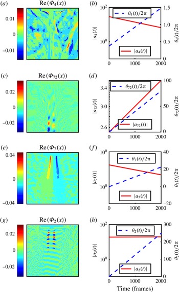
values of 0.1, 0.5, 2.1, 5.2, 11.0, 14.0 and 20.0 show that robust dynamic modes fall into several distinct classes based on their locations, symmetries and dynamics. We outline the classification before presenting the results from the Koopman mode analysis.
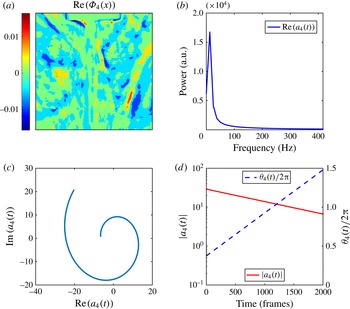
(1) Background modes are spatially disordered, and their primary features lie outside the injector flow. They are transient and decay for all values of
 $J$
. The robust mode 4 of the baseline flow at
 $J=0.1$
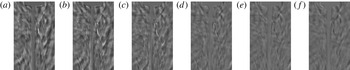
, shown in figure 4, is an example of a background mode. As observed here, the spatial structure of a background mode is disordered. Although these modes are robust within subgroupings of the snapshots in a single experiment, we suspect that their spatial structures differ between experiments.
Background modes (a) are spatially disordered and located outside the injector flow. (b) Their coefficients
 $a(t)$
exhibit low-frequency dynamics. The amplitudes of the modes decay exponentially, as can be observed from the dynamics on the complex plane (c) or from
 $|a(t)|$
(d). The phase of
 $a(t)$
, representing downstream motion of the mode, progresses uniformly, as observed in (d). The remaining figures will be presented in the same format.

(2) Injector modes have a well-defined spatial structure within the injector flow and exhibit high-frequency dynamics. Their coefficients
 $a(t)$
have sharp spectra. For a given subgrouping, their amplitudes exhibit either slow decay or slow growth; as can be seen from figure 16(b), the real part of their eigenvalue is statistically consistent with zero growth. Robust mode 72 of the baseline flow at
 $J=0.1$
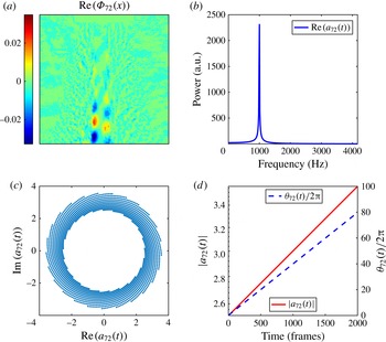
, shown in figure 5, is an example of an injector mode. The projection shown in figure 5(a) supports the assertion that the mode contains successive high- and low-density annular regions, and that the planes of these annuli are, in general, not normal to the symmetry axis. (Injector modes that are symmetric about the axis are also found.) The dynamics of the flow in the complex plane, shown in figure 5(c), lies on an outward moving spiral.
Injector modes (a) are located primarily within the injector flow, and (b) their coefficients
 $a(t)$
exhibit sharp spectra. As observed in (c,d), the amplitude of the mode for the selected subgrouping exhibits slow growth, while the phase progresses uniformly. It should be noted that (c) shows a single trajectory; the illusion of multiple trajectories is caused by the stroboscopic sampling.

(3) Rotating modes are observed for values of
 $J$
larger than 5.2. The reconstruction of the dynamics for one such mode (robust mode 7 for
 $J=11$
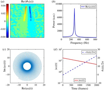
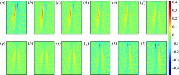
) reveals that the densities of points on either side exhibit antiphase oscillatory behaviour, as observed in figure 8. Since the injector and the flow at the inlet are axially symmetric, this observation indicates that the underlying mode is an azimuthally modulated rotating mode generated via spontaneous symmetry breaking.
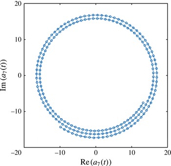
The stroboscopic depiction creates a visual illusion in figure 6(c). The dynamics follows an inward moving spiral and the angular position of the orbit nearly returns to its original value following 93 time steps. Consequently, the set of discrete points on the orbit appears to consist of 93 radial lines. However, joining successive points during a small time interval, as shown in figure 7, reiterates that the orbit is a single inward moving spiral.
Projections of rotating modes (a) are asymmetric, and (b) their coefficients
 $a(t)$
have sharp spectra. As observed in (c,d), they exhibit uniform angular progression. Once again, (c) shows a single trajectory; the illusion of multiple (apparently radial) trajectories is caused by the stroboscopic sampling. Their magnitudes
 $|a(t)|$
exhibit a slow decay. We propose that the underlying three-dimensional flow is an azimuthally modulated rotating mode.

The dynamics of
 $a_{7}(t)$
in the complex plane follows an inward moving spiral. The corresponding motion for growing modes is on outward moving spirals.

Similarly, the orbit shown in figure 5(c) lies on an outward moving spiral. That the motion is outward is confirmed by the (slow) growth of
 $|a_{72}(t)|$
in figure 5(d). Following 24 iterations, the angular and radial positions of the orbit have returned to slightly higher values than in their initial state. Consequently, the stroboscopic image appears to consist of 24 equally spaced arcs.
Reconstruction of the dynamics associated with the rotating mode, presented in figure 8, shows a periodic flipping (left to right) of the high-/low-density regions in the viewing plane. It is uncorrelated to any of the injector modes, as can be established using phase dynamics. Experimental noise and irregularities in the flow cause fluctuations in the coefficients of the dynamic modes. Interestingly, angular changes of the phase-space orbit are highly robust, and the irregularities are restricted to the radial component (Roy et al.
Reference Roy, Hua, Barnhill, Gunaratne and Gord2015). The phase of the coefficient
 $a_{k}(t)$
of a dynamic mode
 ${\it\Phi}_{k}(\boldsymbol{x})$
is defined as
 $$\begin{eqnarray}{\it\theta}_{k}(t)=\tan ^{-1}[\text{Im}(a_{k}(t))/\text{Re}(a_{k}(t))].\end{eqnarray}$$
The relationship between the phases of two dynamic modes can be illustrated using Lissajous figures, such as figure 9, which relate phases of a pair of modes through their sine functions (Roy et al.
Reference Roy, Hua, Barnhill, Gunaratne and Gord2015). Specifically, when the ratio of angular velocities for two phases
 ${\it\theta}_{i}$
and
 ${\it\theta}_{j}$
is a (low-order) rational number, pairs of points
 $\{\sin {\it\theta}_{i}(t),\sin {\it\theta}_{j}(t)\}$
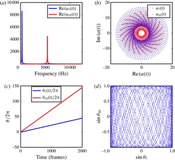
lie on a curve; otherwise, the points fill the space. As an example, figure 9 compares the phase dynamics of the rotating mode with one of the injector modes. Their frequencies (figure 9
a) and phase dynamics (figure 9
c) are not related, and the motion in the Lissajous figure (figure 9
d) is space filling. Thus, it is inferred that the modes are uncorrelated.
Several snapshots of reconstruction of mode 7 for
 $J=11$
, illustrating the antiphase oscillations of the projection: (a) 26.44 ms, (b) 26.48 ms, (c) 26.52 ms, (d) 26.56 ms, (e) 26.60 ms, (f) 26.64 ms, (g) 26.68 ms, (h) 26.72 ms, (i) 26.76 ms, (j) 26.80 ms, (k) 26.84 ms, (l) 26.88 ms.

Comparison of the dynamics of the rotating mode
 ${\it\Phi}_{7}(\boldsymbol{x})$
and an injector mode
 ${\it\Phi}_{10}(\boldsymbol{x})$
for injector flow at
 $J=11$
. Their frequencies (a), complex-plane dynamics (b) and phase dynamics (c) are different. (As in figure 5, (b) shows two trajectories for
 $a_{7}(t)$
(points) and
 $a_{10}(t)$
(solid); the illusion of multiple trajectories is caused by the stroboscopic sampling.) (d) The orbit in the Lissajous figure appears to be a space filling curve. Here,
 ${\it\lambda}_{7}=-16.49+1786.03\text{i}$
, and
 ${\it\lambda}_{10}=-23.96+34127.42\text{i}$
.

(4) Linear response modes are located primarily in the neighbourhood of the injector flow and have an eigenvalue whose imaginary part is the ratio of the acoustic driving frequency and
 $2{\rm\pi}$
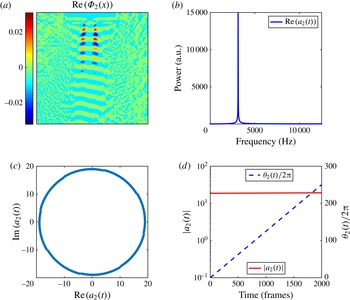
. Figure 10 contains an example of such a mode.
Robust mode 2 for
 $J=0.1$
of the acoustically driven flow is a linear response mode. The imaginary part of its eigenvalue equals the ratio of the driving frequency and
 $2{\rm\pi}$
.

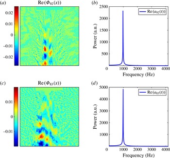
(5) Persistent modes are those observed in PAN driven injector flows that have a structure and period similar to those of corresponding baseline injector modes. For example, as seen from figure 11, mode 83 of the PAN driven flow at
 $J=0.1$
has a structure and dynamics qualitatively similar to mode 92 of the baseline flow. However, the amplitude of the latter is nearly unchanged in time while that of the former is found to decay.
Robust mode 83 of the PAN driven flow, shown in (c), has a structure similar to the robust baseline mode 92 shown in (a). Their spectra, shown in (d) and (b) respectively, are similar as well.

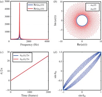
The correlation between persistent modes can be illustrated using their phase dynamics. The frequencies of the time coefficients of the modes (figure 12 a) and their phase dynamics (figure 12 c) are identical. The orbit in the Lissajous figure (figure 12 d) is nearly a closed curve (its width is presumably due to irregularities and experimental noise). Thus, it is inferred that persistent modes are correlated.
The discussion is concluded with a recapitulation (figure 13) of the classes of robust modes identified in injector flows.
The eigenvalues of the two modes compared here are
 ${\it\lambda}=0.05+6155.52\text{i}$
and
 ${\it\lambda}=13.95+6177.75\text{i}$
. Comparison of the dynamics of
 ${\it\Phi}_{92}(t)$
for the baseline flow and
 ${\it\Phi}_{83}(t)$
for the PAN driven flow. The (a) spectra and (c) angular progressions of the dynamics of the two modes are identical. (b) The magnitude
 $|a_{92}(t)|$
of the baseline flow is nearly unchanged (the inner solid line) in time while
 $|a_{83}(t)|$
for the PAN driven flow decays in time (the inward spiralling points). The Lissajous figure, shown in (d), is nearly a closed curve, thus reiterating the correlation between the persistent modes.

The four classes of robust modes found in injector flows and the dynamics of their coefficients: (a,b) a background mode, (c,d) an injector mode, (e,f) a rotating mode and (g,h) a linear response mode.

4.2. Injector flows for low
$J$
(
$J\leqslant 2.1$
)


The major features of the robust modes for injector flows for
 $J\leqslant 2.1$
are similar, and their characteristics will be illustrated using the results for
 $J=0.1$
.
4.2.1. Baseline injector flows for
$\mathit{J}=0.1$

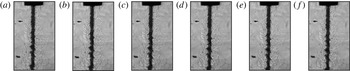
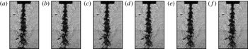
Figure 14 shows a series of images of the baseline flow at
 $J=0.1$
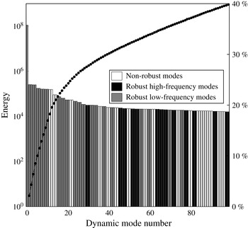
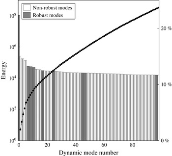
. The injector can be seen at the centre near the top of each image. Figure 15 shows the energies of the 100 DMD modes of the injector flow at
 $J=0.1$
, with energies as defined in § 3.1. It can be observed, as we have already alluded to, that robust and non-robust modes cannot be partitioned using their energies (associated with DMD). The ability to differentiate robust modes from non-robust modes is one of the more significant advantages of DMD. It can be noticed also that the energy of the ‘mean’ mode
 ${\it\Phi}_{0}(\boldsymbol{x})$
is two orders of magnitude larger than the rest. Consequently, the variations of the spatio-temporal velocity field associated with the remaining modes are at least an order of magnitude smaller than those associated with
 ${\it\Phi}_{0}(\boldsymbol{x})$
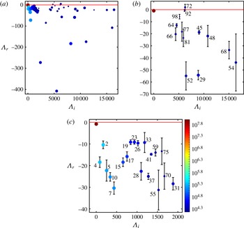
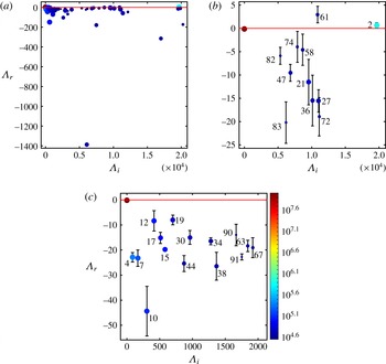
, as can be deduced from the definition of energy (§ 3.1). Figure 16(a) shows the corresponding DMD spectra for modes with non-negative imaginary parts.
Several snapshots of the baseline injector flow at
 $J=0.1$
: (a) 3.96 ms, (b) 4.08 ms, (c) 4.20 ms, (d) 4.32 ms, (e) 4.44 ms and (f) 4.56 ms.

Energies of the 100 DMD modes with the highest energies for the full set of snapshots. Non-reproducible modes of the flow are shown in white. Reproducible modes are partitioned into high-frequency and low-frequency modes, shown in black and grey respectively.

Reproducible modes of the flow are defined using cutoff values
 ${\it\delta}_{I}=36$
,
 ${\it\delta}_{R}=54$
and
 ${\it\Delta}=0.58$
. The modes are partitioned into two groups according to their frequency (imaginary parts of the eigenvalues) and the location of the eigenfunctions. The low-frequency robust modes (
 $\text{Im}({\it\Lambda})\leqslant 2000$
), shown in figure 16(c), are background modes. They are transient; i.e. their amplitudes decay exponentially, as observed in figure 4. The imaginary parts of almost all of the background modes are observed to be (nearly) integer multiples of
 $\text{Im}({\it\Lambda}_{4})$
, suggesting that they are harmonics of
 ${\it\Phi}_{4}(\boldsymbol{x})$
. Together, they will form a single flow constituent. Figure 17 shows several snapshots of the reconstructed spatio-temporal dynamics.
The DMD spectrum of
 $J=0.1$
baseline flow. (a) The 100 modes with the highest energies and positive imaginary parts. The high-frequency (
 $\text{Im}({\it\Lambda}_{i})>2000$
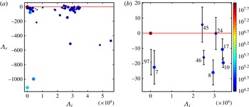
) robust modes, shown in (b), are located near the injector flow. The error bars are standard deviations for a set of eigenvalue real parts from different subgroupings that were identified as representing the same eigenmode. Modes 64, 66, 77, 92, 72, 52, 45, 48, 98, 81 and 68 are asymmetric (e.g. figure 20); modes 29 and 54 are symmetric about the axis. (c) Low-frequency (
 $\text{Im}({\it\Lambda}_{i})\leqslant 2000$
) robust modes that represent the background flow. The colour of the points represents the energies of the modes, according to the colour bar.

Several snapshots of the reconstructed background flow, which lies outside the injector flow and fails to exhibit a well-defined spatial structure: (a) 4 ms, (b) 6 ms, (c) 8 ms, (d) 10 ms, (e) 12 ms and (f) 14 ms.

The high-frequency (
 $\text{Im}({\it\Lambda}_{i})>2000$
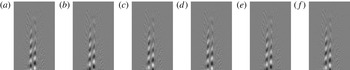
) robust modes, shown in figure 16(b), are located near the injector flow. The dynamic modes associated with each group along with their energies are illustrated in figure 15. The contrast between the background flow and the injector flow (robust mode 48) becomes apparent on comparing the reconstructed flows shown in figures 17 and 18.
Several snapshots of the reconstructed flow for the robust asymmetric mode 48: (a) 4 ms, (b) 4.2 ms, (c) 4.4 ms, (d) 4.6 ms, (e) 4.8 ms and (f) 5 ms. The mode is seen to flow downstream.

For
 $J=0.1$
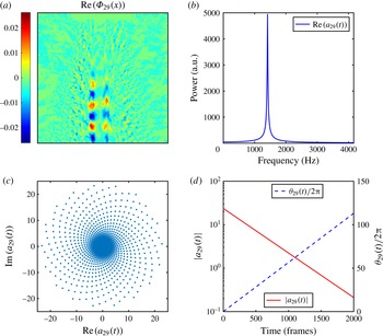
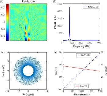
, the robust injector modes, whose spectra are shown in figure 16(b), decay exponentially and are observed to flow downstream. Symmetric and asymmetric injector modes are found, examples of which are given in figures 19 and 20. Since the amplitudes of the modes shown decay in time, the plot of the real versus imaginary parts follows an inward spiralling path.
Robust symmetric mode
 ${\it\Phi}_{29}$
.

Robust asymmetric mode
 ${\it\Phi}_{64}$
.

4.2.2. Acoustically driven injector flows for
$J=0.1$

Figure 21 shows a series of images of the acoustically driven flow at
 $J=0.1$
when the injector is placed at a PAN of the acoustic driving. The flow has considerably more structure than the corresponding baseline flow. The DMD spectrum and robust modes are shown in figure 22. Robust modes were selected using the criteria
 ${\it\delta}_{I}=23$
,
 ${\it\delta}_{R}=15$
and
 ${\it\Delta}=0.4$
. The modes in figure 22(c) capture the spatio-temporal dynamics of the background flow, while those in figure 22(b) represent the injector flow, with some of them having analogues in the baseline flow, as exemplified by the modes shown in figure 11.
Several snapshots of the acoustically driven flow at
 $J=0.1$
when the injector is placed at a PAN of the acoustic driving: (a) 3.96 ms, (b) 4.0 ms, (c) 4.04 ms, (d) 4.08 ms, (e) 4.12 ms and (f) 4.16 ms.

The DMD spectrum for the flow at
 $J=0.1$
when the injector is placed at a PAN of the acoustic driving. (a) The first 100 modes with positive imaginary parts. (b) High-frequency (
 $\text{Im}({\it\Lambda}_{i})>2000$
) robust modes with mode number
 $i$
labelled. The error bars are identical to those defined in figure 16. Mode 2 is the linear response to the driving. (c) The low-frequency robust modes (
 $\text{Im}({\it\Lambda}_{i})\leqslant 2000$
) represent the background flow.

A new robust dynamic mode (mode 2) whose frequency is that of the acoustic driving is found. The imaginary part of
 ${\it\Lambda}_{2}$
is the PAN driving frequency divided by
 $2{\rm\pi}$
, suggesting that it is the linear response of the flow field to the acoustic perturbation. The real part of the eigenvalue is nearly zero, indicating, as seen in figure 10, that
 $a_{2}(t)$
maintains its magnitude in time. The wavelength of the linear response mode is similar to the modulation in the flow seen in figure 21, and the large energy associated with the mode (seen in figure 22) is related to the large amplitude of the modulation.
It can be noticed that the real part of mode 61 is positive, indicating that it grows for the duration of the experiment. We suspect that it saturates at later times; the expectation needs to be verified in longer experimental runs.
4.3. Injector flows for large
$J$
(
$J\geqslant 5.2$
)


The injector flows for
 $J\geqslant 5.2$
present additional robust modes, which are illustrated through the results analysis of the flow for
 $J=11$
.
4.3.1. Baseline injector flows for
$J=11$

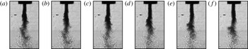
Figure 23 shows several snapshots of the injector flow at
 $J=11$
. It can be noticed that the high-density injector flows diffuse into the ambient fluid earlier at this high
 $J$
. Figure 24 shows the 100 dynamic modes of the flow with the highest energies. As in the case of
 $J=0.1$
, the energy of the mean mode
 ${\it\Phi}_{0}(\boldsymbol{x})$
is more than two orders of magnitude higher than the energies of the remaining modes. It can be observed that there are only a very few robust modes at
 $J=11$
. This is consistent with the presence of large variations in the flow, as illustrated in figure 23.
Several snapshots of the baseline injector flow at
 $J=11$
: (a) 3.96 ms, (b) 4.0 ms, (c) 4.04 ms, (d) 4.08 ms, (e) 4.12 ms and (f) 4.16 ms.

The energies of the 100 DMD modes with the highest energies for the full data set of the injector flow for
 $J=11$
. Non-reproducible modes of the flow are shown in white.

Figure 25(a) shows the DMD spectrum for the flow and figure 25(b) that for the robust modes; as before, the error bars are standard deviations of the set of eigenvalue real parts derived from distinct subgroupings of snapshots selected to represent the same dynamic mode. No robust low-frequency background modes are present in this flow. Furthermore, all injector modes in this flow are asymmetric. As mentioned in § 4.1, when
 $J$
goes beyond 5.2, a rotating mode emerges in the baseline flow. The projection of this mode and the reconstructed dynamics were shown in figures 6 and 8. In addition, the rotating mode is not correlated with any of the injector modes, as illustrated in figure 9.
The DMD spectrum of
 $J=11$
baseline flow. (a) The 100 modes with the highest energies and positive imaginary parts and (b) robust modes. Mode 7 is the new rotating mode, while modes 45, 46, 8, 24, 17 and 10 are asymmetric injector modes.

4.3.2. Acoustically driven injector flows for
$J=11$

Qualitatively, the acoustically driven flow at
 $J=11$
is similar to the corresponding baseline flow. As in the case of low
 $J$
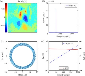
, robust modes of the baseline flow persist when the injector is placed at a PAN of acoustic driving. The driving also initiates a linear response mode, as shown in figure 26. As seen from figure 26(d), the amplitude of
 $a_{1}(t)$
decays slowly for the selected subgrouping; the dynamics of the real versus imaginary parts of
 $a_{1}(t)$
follows an inward spiralling curve.
Linear response mode (mode 1) for PAN driving of the flow at
 $J=11$
. The imaginary part of its eigenvalue is identical to the driving frequency divided by
 $2{\rm\pi}$
.

5. Conclusions
Despite their apparent simplicity, shear coaxial jets can exhibit highly complex dynamical behaviour. Since theoretical analysis of realistic injector flows is difficult, an alternative approach to unravel the complexity is needed. Here, we proposed the use of modal decompositions of high-resolution high-frequency experimental data to perform this task. Teshome (Reference Teshome2012) and Tirunagari et al. (Reference Tirunagari, Hulkkonene, Vuorinen, Kaario and Larmi2012a ,Reference Tirunagari, Vuorinen, Kaario and Larmi b ) implemented modal decompositions using POD. These studies only reported the most significant modes in the flows.
Strongly driven injector flows appear to be highly disordered and contain significant levels of non-reproducible constituents. One disadvantage of POD is the absence of techniques to differentiate these non-reproducible constituents from the robust dynamical features of the flow. In this paper, we used Koopman mode analysis, a natural approach to search for oscillatory modes (Mezic & Banaszuk Reference Mezic and Banaszuk2004; Rowley et al. Reference Rowley, Mezic, Bagheri, Schlatter and Henningson2009; Budišić et al. Reference Budišić, Mohr and Mezić2012; Mezic Reference Mezic, Davis and Moin2013), to decompose injector flows. The difficulty was that even non-cyclic and stochastic constituents of a finite data set may be interpreted as a sum of periodic dynamics. However, the deconvolution of these irregular dynamical facets is non-robust, i.e. they depend on the specific data set. Thus, we proposed an approach for differentiating robust and non-robust features in the flow that is based on identifying the former with reproducible Koopman modes, i.e. those that persist in distinct subgroupings of the data (Roy et al. Reference Roy, Hua, Barnhill, Gunaratne and Gord2015). It was thus possible to study all relevant modes of the flow. It is important to note that only these robust features are expected to be useful in applications such as flow control.
The studies reported here were conducted on injector flows of
 $\text{N}_{2}$
under high pressure into an ambient
 $\text{N}_{2}$
background. The flows were observed with shadowgraph imaging using diffuse backscattering. The high-density injector flows could be observed as darker regions of the visual field. Koopman mode analysis of the density field in baseline flows (those not subjected to additional perturbations) and acoustically excited flows revealed several classes of robust dynamic modes. The modulations of the density field imposed by each of these modes were at least an order of magnitude smaller than the spatial variations in the time-averaged flow.
Several distinct groups of robust dynamic modes characterized by their spatial locations and dynamics were identified in the baseline flows. The first group contained a set of low-frequency excitations located outside the primary injector flow that exhibited rapid decay, as can be observed in figure 4 and the Koopman spectrum in figure 16(c). Reconstruction of the flow associated with background modes (figure 17) showed that this flow constituent has no well-defined structure. Although background modes are common between different subgroupings of snapshots in a single experiment, it is expected that they will differ among experiments. Background modes are not found for larger values of the control parameter
 $J$
, presumably because they have decayed to insignificant levels during the experiment.
The second group of modes are referred to as injector modes because of their location near the primary injector flow. Unlike background modes, they have a well-defined structure, an example of which is shown in figure 5; they are high-frequency modes, propagate along the flow (see figure 18) and decay at a significantly slower rate. The wavelength of injector modes is comparable to the modulations of the flow, seen in figure 14, and is likely to be the origin of the latter. The spectrum of injector modes and their error estimates, shown in figure 16(b), suggest that some of these may persist beyond the initial transients. This suggestion needs to be validated in longer experimental runs. The broad features of injector modes remain unchanged under acoustic perturbation (figure 22) and for higher values of
 $J$
(figure 25). While injector modes for small
 $J$
can be either symmetric (figure 19) or asymmetric (figure 20) in the viewing plane, those for large values of
 $J$
are antisymmetric. It is possible that the high-/low-density regions in these modes are spirals. They are the only modes reported by Teshome (Reference Teshome2012).
Acoustic driving generates additional small-wavelength modulations of the injector flow, as can be seen in figure 21. These appear to be caused by a new robust mode, which we referred to as a linear response mode; the imaginary part of its eigenvalue is identical to the driving frequency (divided by
 $2{\rm\pi}$
). Their dynamics exhibits a very sharp spectrum, and their magnitude is (nearly) uniform in time, as seen from figures 10 and 26. For the acoustic driving studied, the spatial periodicity of the linear response mode is smaller than that of injector modes, resulting in the smaller wavelength modulations observed in figure 21. As seen from figure 22, the linear response mode has a large energy, which is correlated with the increased amplitude of modulations of the flow. Linear response modes are found for PAN driven flows at all values of
 $J$
.
A class of robust dynamic modes of the baseline flow retain their structure and dynamical features under acoustic perturbation. A pair of such modes is shown in figure 11, and the comparison of dynamics of a baseline mode and the corresponding PAN driven persistent mode is shown in figure 12. These modes, referred to as persistent modes, were found for all values of
 $J$
studied.
The most interesting class of modes was termed rotating modes, as shown in figure 6, and only observed for
 $J>5.2$
. The projection of their density fields exhibits antiphase oscillatory behaviour. The reconstruction of the spatio-temporal dynamics, illustrated using several snapshots in figure 8, highlights a periodic flipping of the high-/low-density regions. Since the injector and the inlet flow are axisymmetric and the viewing plane has no special stature, the flipping observed in the viewing plane can only be described as a projection of an azimuthally modulated rotating mode, generated via a spontaneous symmetry breaking (Cross & Hohenberg Reference Cross and Hohenberg1993) similar to the rotating modes in uniform flame fronts (Palacios et al.
Reference Palacios, Gunaratne, Gorman and Robbins1997). The modes persist under acoustic perturbation, although in this case the system is not axisymmetric, and the symmetry breaking may not be spontaneous.
The roles played by robust modes at different values of
 $J$
, the outer-to-inner-jet momentum ratio, can be quantified by figures 15 and 24. Injector flows for small values of
 $J$
(when the outer-jet momentum is relatively large) contain only a few non-robust modes, while those for large values of
 $J$
consist mostly of non-robust modes. The implication is that large-
 $J$
flows are more irregular, an observation consistent with figures 14 and 23. The energy distributions also reaffirm that it may not be possible to differentiate robust and non-robust flow constituents using their energies alone.
The modal decompositions of injector flows presented here highlight the need for additional investigations. One issue is to identify robust Koopman modes that persist beyond the initial transient stage, i.e. those relevant for long-term flows. For example, our analysis of injector flows suggests that while the background modes are transient, many of the injector modes will persist. The task of differentiating the two groups can be implemented in one of two ways. The first is to conduct and analyse longer experimental runs where transients have decayed. An alternative computational approach is to conduct a sparsity-promoting DMD introduced recently (Jovanovic, Schimid & Nichols Reference Jovanovib́, Schmid and Nichols2014). Sparsity-promoting DMD performs the extraction of dynamic modes associated with persistent flows, even when transients have larger energy.
The formation of rotating modes for
 $J\geqslant 5.2$
is another extremely interesting observation and requires further investigations. It would be especially important to validate the mode with supplementary measurements, study its onset in detail, and analyse flows appearing in injectors with other geometries and under different classes of acoustic perturbations. Finally, it will be beneficial to determine whether additional classes of dynamic modes are present in the corresponding combustion flows.
Acknowledgement
Funding for this research was provided by the Air Force Research Laboratory under contract nos. FA8650-13-C-2440 and FA9300-13-M-1503. The paper has been cleared for public release by the Air Force Research Laboratory (no. 88ABW-2015-3171).