1. Introduction
Gravity currents and other shallow flows through porous media play a central role in a range of geophysical and industrial problems, ranging from the seepage of contaminated plumes or the spread of fresh water lenses above saline aquifers to the displacement of one fluid by another in oil reservoirs to enhance recovery (Bear Reference Bear1988; Phillips Reference Phillips2009). The fluid mechanics of such flows are often explored under the assumption that the porous matrix does not deform due to fluid flow. However, when flow-induced pressure gradients are high, or when the solid matrix is relatively soft, as in some biological problems (e.g. Mow, Holmes & Lai Reference Mow, Holmes and Lai1984), the deformation of the matrix can be significant. Our goal in the current paper is to formulate a model of poro-elastic flow in a shallow layer, where elastic deformation of the porous matrix is coupled to the flow of fluid through it. We apply the model to study the dynamics of axisymmetric poro-elastic gravity currents.
Specific motivation for this problem comes from observations of surface displacements at the
 $\text{CO}_{2}$
storage sites at In Salah in the Algerian desert (Ringrose et al.
Reference Ringrose, Mathieson, Wright, Selama, Hansen, Bissell, Saoula and Midgley2013). Geological sequestration has been widely proposed as a means of countering atmospheric emissions of
 $\text{CO}_{2}$
through the injection of supercritical
 $\text{CO}_{2}$
into (typically) water-saturated porous rock (e.g. Zhang Reference Zhang2013; Huppert & Neufeld Reference Huppert and Neufeld2014). Being less dense than the ambient water, injected
 $\text{CO}_{2}$
rises and spreads as a gravity current below the impermeable overburden of the porous reservoir (Boait et al.
Reference Boait, White, Bickle, Chadwick, Neufeld and Huppert2012). At In Salah, approximately 4 million tonnes of
 $\text{CO}_{2}$
were sequestered between 2004 and 2011 into a sandstone layer, roughly 20 m thick and located approximately 2 km underground (Ringrose et al.
Reference Ringrose, Atbi, Mason, Espinassous, Myhrer, Iding, Mathieson and Wright2009, Reference Ringrose, Mathieson, Wright, Selama, Hansen, Bissell, Saoula and Midgley2013). Around the sites of injection, vertical surface displacements of the order of centimetres have been detected by interferometric synthetic aperture radar (InSAR) measurements (Onuma & Ohkawa Reference Onuma and Ohkawa2009; Rucci, Vasco & Novali Reference Rucci, Vasco and Novali2013). These observations highlight how the injection and subsequent spread of
 $\text{CO}_{2}$
has deformed the porous sandstone layer, much as fluid pumping in other hydrological contexts generates subsidence or uplift (e.g. Bear & Corapcioglu Reference Bear and Corapcioglu1981a
,Reference Bear and Corapcioglu
b
). The InSAR measurements have been proposed as a monitor of the progress of the
 $\text{CO}_{2}$
current (Ringrose et al.
Reference Ringrose, Atbi, Mason, Espinassous, Myhrer, Iding, Mathieson and Wright2009), even though the detailed relation between the uplift at the surface and the location of the underlying current has not yet been fully understood.
The large horizontal and thin vertical extent that is typical of sequestration sites is well suited to the conventional shallow-layer modelling of gravity currents (e.g. Huppert & Woods Reference Huppert and Woods1995; Lyle et al.
Reference Lyle, Huppert, Hallworth, Bickle and Chadwick2005; Nordbotten & Celia Reference Nordbotten and Celia2006). Despite this, most existing studies in geological engineering use standard geomechanical models coupled with reservoir-type simulations (Rutqvist, Vasco & Myer Reference Rutqvist, Vasco and Myer2010; Bissell et al.
Reference Bissell, Vasco, Atbi, Hamdani, Okwelegbe and Goldwater2011; Rutqvist Reference Rutqvist2012). These studies have provided predictions for uplift and rates of spread that have been compared with the observations from In Salah, highlighting how local topography and fractures have helped to guide the flow of
 $\text{CO}_{2}$
. They do not, however, focus on the detailed fluid mechanics of spreading poro-elastic currents, nor extract the dependence on the physical parameters of the problem, which are the goals of the current paper.
In this paper we formulate a poro-elastic model for axisymmetric flow in a shallow layer that combines Biot’s theory (e.g. Detournay & Cheng Reference Detournay and Cheng1993; Coussy Reference Coussy2004) with shallow-layer scalings following standard gravity-current theory (e.g. Huppert & Woods Reference Huppert and Woods1995). Our methodology is similar to that adopted for other subsidence and pumping problems in hydrology (e.g. Gibson, Schiffman & Pu Reference Gibson, Schiffman and Pu1970; Bear & Corapcioglu Reference Bear and Corapcioglu1981a ,Reference Bear and Corapcioglu b ,Reference Bear and Corapcioglu c ) and industrial filtration (Barry, Mercer & Zoppou Reference Barry, Mercer and Zoppou1997). In a biological context, a similar poro-elastic framework has been used to describe cell dynamics (Charras, Mitchison & Mahadevan Reference Charras, Mitchison and Mahadevan2009; Moeendarbary et al. Reference Moeendarbary, Valon, Fritzsche, Harris, Moulding, Thrasher, Stride, Mahadevan and Charras2013) and tissue swelling or oedemas (Simon et al. Reference Simon, Liable, Pflaster, Yuan and Krag1996). Indeed, flow-induced deformation of shallow poro-elastic layers is central to a number of biological problems, with the indentation of tissue layers such as cartilage playing a key role in, for example, the lubrication of joints (see Mak, Lai & Mow Reference Mak, Lai and Mow1987; Mow et al. Reference Mow, Gibbs, Lai, Zhu and Athanasiou1989; Jensen et al. Reference Jensen, Glucksberg, Sachs and Grotberg1994; Sachs et al. Reference Sachs, Glucksberg, Jensen and Grotberg1994; Barry & Holmes Reference Barry and Holmes2001).
Our current formulation generalizes previous models in two notable ways: first, we allow for two fluids of different density, one displacing the other as it spreads under gravity (we assume that the medium is fully saturated). Second, we assume that the poro-elastic layer lies between a rigid base and a flexible overburden, both of which are impermeable, and that the poro-elastic material cannot slide freely at either surface. Poro-elastic deformations are therefore significantly constrained by the shallow geometry. Both features provide the conceptual framework for application to uplift in
 $\text{CO}_{2}$
sequestration.
We complement our theoretical model with a series of idealized laboratory experiments. Previous experimentalstudies using deformable media havepredominantly been concerned with one-dimensional compression tests, using materials such as artificial sponges (Parker, Mehta & Caro Reference Parker, Mehta and Caro1987; Lanir, Sauob & Maretsky Reference Lanir, Sauob and Maretsky1990), synthetic fibres (Barabadi et al. Reference Barabadi, Nathan, Jen and Wu2009) and biological tissue (Eisenberg & Grodzinsky Reference Eisenberg and Grodzinsky1987). In more recent experiments, MacMinn, Dufresne & Wettlaufer (Reference MacMinn, Dufresne and Wettlaufer2015) used a mono-layer of small spherical polyacrylamide hydrogel particles to study flow-induced deformation of an idealized two-dimensional poro-elastic medium. Such hydrogels are convenient materials for poro-elastic experiments, being relatively inexpensive and straightforward to prepare and visualize. We used similar hydrogel particles, fully saturated in water, to provide a rough experimental analogue of the theoretical model.
The paper is laid out as follows. In § 2, we formulate the poro-elastic shallow-layer framework to construct our model. The model takes the form of coupled evolution equations for the height of the injected fluid current and the uplift of the flexible overburden owing to deformation of the medium. In § 3, we discuss numerical results of the model with a constant flux of injection. In § 4, we present an asymptotic analysis of the model and deduce scaling relationships for the spread of the injected current and of the uplift. In § 5, we present the results of the laboratory experiments. The main conclusions and implications of this work are summarized in § 6.
2. Theoretical modelling
2.1. Governing equations
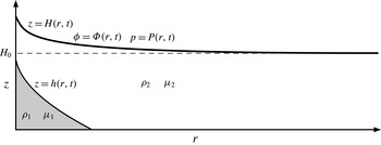
We consider flow through a deformable porous medium in an axisymmetric geometry described by cylindrical polar coordinates
 $(r,z)$
(figure 1). The porous layer sits on top of a rigid, impermeable, flat base located at
 $z=0$
and extends up to a height
 $z=H(r,t)$
, where it is overlain by a heavy flexible sheet. The layer initially has uniform depth
 $H=H_{0}$
. The solid matrix has constant density
 ${\it\rho}_{s}$
, and the medium is initially fully saturated with ambient fluid of density
 ${\it\rho}_{2}\leqslant {\it\rho}_{s}$
and viscosity
 ${\it\mu}_{2}$
. Another fluid of density
 ${\it\rho}_{1}$
and viscosity
 ${\it\mu}_{1}$
is injected into the medium and spreads under gravity. Following standard gravity-current theory (Huppert & Woods Reference Huppert and Woods1995), we take
 ${\it\rho}_{1}\geqslant {\it\rho}_{2}$
, so that the injected fluid spreads along the bottom of the porous layer; the spreading of a lighter fluid injection along the top of the medium can be modelled in an analogous fashion. The interface between the two fluids is denoted by
 $z=h(r,t)$
. The amount of fluid within a representative volume element of the material is given by the porosity
 ${\it\phi}(r,z,t)$
, which varies in both space and time. The pore-averaged velocity of the fluid and solid phases are
 $\boldsymbol{u}_{\boldsymbol{f}}=(u_{f},w_{f})$
and
 $\boldsymbol{u}_{\boldsymbol{s}}=(u_{s},w_{s})$
, respectively. Both phases are assumed to be incompressible, such that their densities are constant.
A schematic showing the depth
 $h(r,t)$
of the injected fluid and the uplift
 $H(r,t)$
of the overburden, associated with an injected flux
 $Q$
at
 $r=0$
. The porosity and fluid pressure at
 $z=H$
are given by
 ${\it\phi}={\it\Phi}(r,t)$
and
 $p=P(r,t)$
, respectively. Before any fluid is injected,
 $H=H_{0}$
,
 ${\it\Phi}={\it\Phi}_{0}$
and
 $P=\mathscr{P}$
, where
 $\mathscr{P}$
is the overburden pressure.

The governing equations for flow and deformation in a poro-elastic medium are continuity for the liquid and the solid phases, Darcy’s law and a global momentum balance:
 $$\begin{eqnarray}\frac{\partial {\it\phi}}{\partial t}+\boldsymbol{{\rm\nabla}}\boldsymbol{\cdot }({\it\phi}\boldsymbol{u}_{\boldsymbol{f}})=0,\quad \frac{\partial }{\partial t}(1-{\it\phi})+\boldsymbol{{\rm\nabla}}\boldsymbol{\cdot }[(1-{\it\phi})\boldsymbol{u}_{\boldsymbol{s}}]=0,\end{eqnarray}$$
 $$\begin{eqnarray}\displaystyle & \displaystyle {\it\phi}(\boldsymbol{u}_{\boldsymbol{f}}-\boldsymbol{u}_{\boldsymbol{s}})=-\frac{k}{{\it\mu}_{i}}(\boldsymbol{{\rm\nabla}}p+{\it\rho}_{i}g\boldsymbol{e}_{z}), & \displaystyle\end{eqnarray}$$
 $$\begin{eqnarray}\displaystyle & \displaystyle \boldsymbol{{\rm\nabla}}\boldsymbol{\cdot }[(1-{\it\phi}){\bf\sigma}-{\it\phi}p\unicode[STIX]{x1D644}]=[{\it\rho}_{i}{\it\phi}+{\it\rho}_{s}(1-{\it\phi})]g\boldsymbol{e}_{z}, & \displaystyle\end{eqnarray}$$
 $k({\it\phi})$
is the permeability of the medium,
 $p$
is the pore pressure,
 $g$
is the gravitational acceleration,
 ${\bf\sigma}$
is the phase-averaged solid stress tensor,
 $\unicode[STIX]{x1D644}$
is the identity tensor and
 $\boldsymbol{e}_{z}$
is the unit vector in the
 $z$
direction. The subscript
 $i$
refers to the injected (
 $i=1$
) or ambient (
 $i=2$
) fluid.
The equations are closed by a constitutive law for the solid stress. More commonly, as suggested by Terzaghi’s principle in soil mechanics (e.g. Wang Reference Wang2000), the closure is a constitutive law for the ‘effective’ stress tensor
 ${\bf\sigma}_{\boldsymbol{e}}$
of the medium, which is the difference between the total volume-averaged stress and the pore pressure,
 ${\bf\sigma}_{\boldsymbol{e}}=({\bf\sigma}+p\unicode[STIX]{x1D644})(1-{\it\phi})$
. The momentum balance (2.3) can be re-written in terms of
 ${\bf\sigma}_{\boldsymbol{e}}$
as
 $$\begin{eqnarray}\boldsymbol{{\rm\nabla}}\boldsymbol{\cdot }({\bf\sigma}_{\boldsymbol{e}}-p\unicode[STIX]{x1D644})=[{\it\rho}_{i}{\it\phi}+{\it\rho}_{s}(1-{\it\phi})]g\boldsymbol{e}_{z}.\end{eqnarray}$$
In general, an elastic constitutive law for
 ${\bf\sigma}_{\boldsymbol{e}}$
takes the form
 $$\begin{eqnarray}{\bf\sigma}_{\boldsymbol{e}}={\bf\sigma}_{\boldsymbol{e}}(\boldsymbol{{\rm\nabla}}{\bf\xi}),\end{eqnarray}$$
where
 ${\bf\xi}=({\it\xi},{\it\zeta})$
is the deformation of the medium away from a reference state with constant porosity
 ${\it\Phi}_{0}$
. The deformation, which we describe in terms of Eulerian variables, is related to the solid velocity
 $\boldsymbol{u}_{\boldsymbol{s}}$
via the convective derivative
 $$\begin{eqnarray}\boldsymbol{u}_{\boldsymbol{s}}=\left(\frac{\partial }{\partial t}+\boldsymbol{u}_{\boldsymbol{s}}\boldsymbol{\cdot }\boldsymbol{{\rm\nabla}}\right){\bf\xi}.\end{eqnarray}$$
In this paper, following standard formulations of Biot’s theory (e.g. Detournay & Cheng Reference Detournay and Cheng1993), we adopt a linear elastic constitutive law (i.e. Hooke’s law) for the effective stress (2.5),
 $$\begin{eqnarray}{\bf\sigma}_{\boldsymbol{e}}=\left(K-{\textstyle \frac{2}{3}}G\right)(\boldsymbol{{\rm\nabla}}\boldsymbol{\cdot }{\bf\xi})\unicode[STIX]{x1D644}+G[(\boldsymbol{{\rm\nabla}}{\bf\xi})+(\boldsymbol{{\rm\nabla}}{\bf\xi})^{\text{T}}],\end{eqnarray}$$
where
 $K$
and
 $G$
are the bulk and shear moduli, which are assumed to be constant. Note that these moduli are properties of the porous medium, rather than of the pure solid alone. In fact, in the shallow-layer limit introduced in § 2.2, (2.7) simplifies significantly and could be replaced by a more general nonlinear constitutive law without undue extra complication.
2.2. Dimensionless shallow-layer scalings
We suppose that the vertical extent
 $H_{0}$
of the porous layer is much less than the characteristic radial length scale
 $L$
of the flow, so that
 $H_{0}\ll L$
. Scaling analysis of the continuity equation for the fluid phase (2.1a
) indicates that
 $w_{f}\ll u_{f}$
. However, we cannot make the same deduction for the solid velocity in (2.1b
): under the assumption that the solid cannot freely slip on the boundaries, there must be a frictional balance between normal and shear stress there, which indicates that
 ${\it\xi}\sim {\it\zeta}$
and thus
 $u_{s}\sim w_{s}$
. The relative magnitude of the fluid and solid velocities can be determined by (2.1), which indicates that
 $w_{s}\sim w_{f}$
, and so
 $u_{s}\ll u_{f}$
.
We introduce the following dimensionless quantities:
 $$\begin{eqnarray}r^{\ast }=\frac{r}{L},\quad (z^{\ast },{\it\xi}^{\ast },{\it\zeta}^{\ast })=\frac{1}{H_{0}}(z,{\it\xi},{\it\zeta}),\quad {\it\rho}_{i}^{\ast }=\frac{{\it\rho}_{i}}{{\it\rho}_{s}},\quad p^{\ast }=\frac{p}{{\it\rho}_{s}gH_{0}},\quad k^{\ast }=\frac{k}{k_{0}},\end{eqnarray}$$
 $$\begin{eqnarray}u_{f}^{\ast }=\frac{u_{f}}{U},\quad (w_{f}^{\ast },u_{s}^{\ast },w_{s}^{\ast })=\frac{L}{UH_{0}}(w_{f},u_{s},w_{s}),\quad t^{\ast }=\frac{Ut}{L},\end{eqnarray}$$
where
 $U={\it\rho}_{s}gk_{0}H_{0}/{\it\mu}_{1}L$
and
 $k_{0}=k({\it\Phi}_{0})$
is a characteristic permeability scale. For notational convenience, we also define the scaled dimensionless density differences and the viscosity, or mobility, ratio,
 $$\begin{eqnarray}\widehat{{\it\rho}}_{1}=(1-{\it\Phi}_{0})\frac{{\it\rho}_{s}-{\it\rho}_{1}}{{\it\rho}_{s}},\quad \widehat{{\it\rho}}_{2}=(1-{\it\Phi}_{0})\frac{{\it\rho}_{s}-{\it\rho}_{2}}{{\it\rho}_{s}},\end{eqnarray}$$
 $$\begin{eqnarray}{\rm\Delta}{\it\rho}=\frac{{\it\rho}_{1}-{\it\rho}_{2}}{{\it\rho}_{s}}=\widehat{{\it\rho}}_{2}-\widehat{{\it\rho}}_{1},\quad M=\frac{{\it\mu}_{1}}{{\it\mu}_{2}}.\end{eqnarray}$$
For the arrangement depicted in figure 1,
 $0\leqslant \widehat{{\it\rho}}_{1}\leqslant \widehat{{\it\rho}}_{2}\leqslant 1$
and
 ${\rm\Delta}{\it\rho}\geqslant 0$
. At this stage, the radial length scale
 $L$
is not prescribed by the dynamics, and in the absence of an external radial scale in the boundary conditions it remains undetermined. In such a situation, we expect that the equations permit a similarity solution, as we in fact find to be the case and discuss in § 3.
In the shallow-layer framework, we retain only the leading-order terms in
 $H_{0}/L$
. The dimensionless shallow-layer continuity equations are given from (2.1) by
 $$\begin{eqnarray}\frac{\partial {\it\phi}}{\partial t^{\ast }}=-\frac{1}{r^{\ast }}\frac{\partial }{\partial r^{\ast }}(r^{\ast }{\it\phi}u_{f}^{\ast })-\frac{\partial }{\partial z^{\ast }}({\it\phi}w_{f}^{\ast })=\frac{\partial }{\partial z^{\ast }}[(1-{\it\phi})w_{s}^{\ast }].\end{eqnarray}$$
From (2.2) and the shallow-layer scalings, the pore pressure is hydrostatic and the fluid velocity is given by the horizontal component of Darcy’s law,
 $$\begin{eqnarray}\frac{\partial p^{\ast }}{\partial z^{\ast }}=-{\it\rho}_{i}^{\ast },\quad {\it\phi}u_{f}^{\ast }=\left\{\begin{array}{@{}ll@{}}-k^{\ast }\hspace{2.22198pt}\partial p^{\ast }/\partial r^{\ast }\quad & \text{for }0<z^{\ast }<h^{\ast },\\ -Mk^{\ast }\hspace{2.22198pt}\partial p^{\ast }/\partial r^{\ast }\quad & \text{for }h^{\ast }<z^{\ast }<H^{\ast }.\end{array}\right.\end{eqnarray}$$
The vertical momentum balance in (2.4), together with the linearly elastic rheology (2.7), reduces to an ordinary differential equation for the vertical displacement
 ${\it\zeta}^{\ast }$
, given by
 $$\begin{eqnarray}E\frac{\partial ^{2}{\it\zeta}^{\ast }}{\partial z^{\ast 2}}-\frac{\partial p^{\ast }}{\partial z^{\ast }}=[{\it\rho}_{i}^{\ast }{\it\phi}+(1-{\it\phi})],\end{eqnarray}$$
where
 $$\begin{eqnarray}E=\frac{K+4G/3}{{\it\rho}_{s}gH_{0}}\end{eqnarray}$$
is a dimensionless elastic modulus or stiffness of the medium.
In the shallow framework, the closure relationship (2.6) becomes one-dimensional and gives an explicit equation for the solid velocity:
 $w_{s}^{\ast }=\partial {\it\zeta}^{\ast }/\partial t^{\ast }/(1-\partial {\it\zeta}^{\ast }/\partial z^{\ast })$
. Substitution of this expression into the equation of continuity of the solid phase (2.12b
) gives, after rearranging,
 $$\begin{eqnarray}\left(\frac{\partial }{\partial t^{\ast }}+w_{s}^{\ast }\frac{\partial }{\partial z^{\ast }}\right)\left(\frac{1-\partial {\it\zeta}^{\ast }/\partial z^{\ast }}{1-{\it\phi}}\right)=0,\end{eqnarray}$$
or, after integration,
 $$\begin{eqnarray}\frac{\partial {\it\zeta}^{\ast }}{\partial z^{\ast }}=\frac{{\it\phi}-{\it\Phi}_{0}}{1-{\it\Phi}_{0}}\end{eqnarray}$$
given that
 ${\it\Phi}_{0}$
is the constant porosity of the reference state. Equations (2.13a
), (2.14) and (2.17) can be combined to eliminate
 ${\it\zeta}^{\ast }$
and
 $p^{\ast }$
:
 $$\begin{eqnarray}\frac{\partial {\it\phi}}{\partial z^{\ast }}=\frac{\widehat{{\it\rho}}_{i}(1-{\it\phi})}{E}.\end{eqnarray}$$
The horizontal deformation
 ${\it\xi}^{\ast }$
does not appear in the equations given above, which is a result of the linear elastic constitutive law (2.7). For a more general nonlinear constitutive law, the leading-order elastic stress might also feature the strain component
 $\partial {\it\xi}/\partial z$
, which could be recovered from the leading-order horizontal stress balance in (2.4).
2.3. Boundary and initial conditions
For the remainder of the paper, we drop the starred notation that identifies the dimensionless variables.
2.3.1. Surface and interface conditions
The boundary conditions on the impermeable and immobile base of the medium are
 $$\begin{eqnarray}w_{f}=w_{s}={\it\zeta}=0\quad \text{at }z=0,\end{eqnarray}$$
while the interface
 $z=h(r,t)$
between the two fluids satisfies the kinematic condition
 $$\begin{eqnarray}\frac{\partial h}{\partial t}+u_{f}|_{z=h}\frac{\partial h}{\partial r}=w_{f}|_{z=h}.\end{eqnarray}$$
At the upper surface of the medium, we assume that both the solid and the fluid phases remain in contact with the overburden at all times. In the shallow-layer limit, the corresponding kinematic conditions are
 $$\begin{eqnarray}\frac{\partial H}{\partial t}+u_{f}|_{z=H}\frac{\partial H}{\partial r}=w_{f}|_{z=H}\quad \text{and}\quad \frac{\partial H}{\partial t}=w_{s}|_{z=H}.\end{eqnarray}$$
A balance of normal stress at the upper surface of the medium also gives
 $$\begin{eqnarray}-p+\boldsymbol{e}_{\boldsymbol{z}}\boldsymbol{\cdot }{\bf\sigma}_{\boldsymbol{e}}\boldsymbol{\cdot }\boldsymbol{e}_{\boldsymbol{z}}=-\mathscr{P}\quad \text{at }z=H,\end{eqnarray}$$
where
 $\mathscr{P}$
is the dimensionless normal stress imposed by the overburden. Given the constitutive equation (2.7) and the shallow-layer scalings, we have
 $\boldsymbol{e}_{\boldsymbol{z}}\boldsymbol{\cdot }{\bf\sigma}_{\boldsymbol{e}}\boldsymbol{\cdot }\boldsymbol{e}_{\boldsymbol{z}}=E\partial {\it\zeta}/\partial z$
, and so, from (2.17), the normal-stress balance reduces to
 $$\begin{eqnarray}p-\mathscr{P}=E\frac{{\it\phi}-{\it\Phi}_{0}}{1-{\it\Phi}_{0}}\quad \text{at }z=H.\end{eqnarray}$$
The stress
 $\mathscr{P}$
in general contains contributions from the bending and tension of the overburden, as well as from gravity. Here, we neglect the elastic response of the overburden and take
 $\mathscr{P}$
to be a constant, given by the weight of the overburden per unit area.
2.3.2. Injection and far-field conditions
Fluid is injected into the medium as a point source at the origin with a flux
 $Q(t)$
, while no ambient fluid is removed. Thus,
 $$\begin{eqnarray}\lim _{r\rightarrow 0}\int _{0}^{h}r{\it\phi}u_{f}\,\text{d}z=\frac{Q}{2{\rm\pi}},\quad \lim _{r\rightarrow 0}\int _{h}^{H}r{\it\phi}u_{f}\,\text{d}z=0,\end{eqnarray}$$
where we note that the dimensional flux is
 $QH_{0}LU=Q{\it\rho}_{s}gk_{0}H_{0}^{2}/{\it\mu}_{1}$
.
For the analysis of the model, we assume that the domain extends infinitely in the radial direction with
 $$\begin{eqnarray}h\rightarrow 0,\quad H\rightarrow 1,\quad \text{as }r\rightarrow \infty .\end{eqnarray}$$
For laboratory experiments and numerical computations the extent of the domain must be finite. In these cases, we consider an impermeable boundary where
 $\partial H/\partial r=\partial h/\partial r=0$
at
 $r=r_{edge}\gg 1$
. We will be primarily interested in times before significant pressure signals from the injection have reached the edge of the domain, and so this far-field boundary condition plays little role in the dynamics.
2.3.3. Initial conditions
The medium has initial depth
 $H(r,t=0)=1$
, and is fully saturated with ambient fluid such that
 $h(r,t=0)=0$
. The initial porosity profile
 ${\it\phi}(r,z,t=0)={\it\phi}_{0}(z)$
can be calculated from the integral of (2.18), and is given by
 $$\begin{eqnarray}{\it\phi}_{0}=1-(1-{\it\Phi}_{0})\text{e}^{(1-z)\widehat{{\it\rho}}_{2}/E},\end{eqnarray}$$
where we have fixed the reference state
 ${\it\phi}(t=0,z=1)={\it\Phi}_{0}$
to coincide with the initial condition at the surface. Note that if the stiffness
 $E$
is sufficiently small, (2.26) unphysically predicts that the porosity falls below zero at a finite depth within the layer. In a physical setting, it is likely that the assumption of linear elasticity would break down well before this limit is reached. In practice, we will only consider parameter settings in which the porosity is everywhere significantly larger than zero, and so we ignore the possibility of vanishing porosity.
2.4. The dimensionless model
By integrating (2.13a ), we find that the hydrostatic pore pressure is
 $$\begin{eqnarray}p(r,z,t)=\left\{\begin{array}{@{}ll@{}}P+{\it\rho}_{2}(H-h)+{\it\rho}_{1}(h-z)\quad & \text{for }0<z<h,\\ P+{\it\rho}_{2}(H-z)\quad & \text{for }h<z<H,\end{array}\right.\end{eqnarray}$$
where
 $P(r,t)$
is the (unknown) surface pore pressure. The porosity distribution is given by integrating (2.18), which yields
 $$\begin{eqnarray}{\it\phi}(r,z,t)=\left\{\begin{array}{@{}ll@{}}1-(1-{\it\Phi})\text{e}^{(H-h)\widehat{{\it\rho}}_{2}/E+(h-z)\widehat{{\it\rho}}_{1}/E}\quad & \text{for }0<z<h,\\ 1-(1-{\it\Phi})\text{e}^{(H-z)\widehat{{\it\rho}}_{2}/E}\quad & \text{for }h<z<H,\end{array}\right.\end{eqnarray}$$
where
 ${\it\Phi}(r,t)$
is the porosity at
 $z=H$
. The pressure
 $P$
and porosity
 ${\it\Phi}$
are linked by the continuity of normal stress at
 $z=H$
(2.23), which gives
 $$\begin{eqnarray}P-\mathscr{P}=E\frac{{\it\Phi}-{\it\Phi}_{0}}{1-{\it\Phi}_{0}}.\end{eqnarray}$$
The porosity
 ${\it\Phi}$
at the upper surface is also related to the heights
 $h$
and
 $H$
via the kinematic condition (2.21), which can be combined with the vertical integral of the continuity equations (2.12) to give a conservation law for the solid phase in any vertical slice,
 $$\begin{eqnarray}\frac{\partial }{\partial t}\left[\int _{0}^{H}(1-{\it\phi})\,\text{d}z\right]=0,\quad \text{or}\quad \int _{0}^{H}(1-{\it\phi})\,\text{d}z=\int _{0}^{1}(1-{\it\phi}_{0})\,\text{d}z.\end{eqnarray}$$
Using (2.26) and (2.28), we then find the following expression for the surface porosity
 ${\it\Phi}[h(r,t),H(r,t)]$
:
 $$\begin{eqnarray}\frac{1-{\it\Phi}}{(1-{\it\Phi}_{0})[\text{e}^{\widehat{{\it\rho}}_{2}/E}-1]}=\left\{\text{e}^{(H-h)\widehat{{\it\rho}}_{2}/E}-1+\frac{\widehat{{\it\rho}}_{2}}{\widehat{{\it\rho}}_{1}}[\text{e}^{h\widehat{{\it\rho}}_{1}/E}-1]\text{e}^{(H-h)\widehat{{\it\rho}}_{2}/E}\right\}^{-1}.\end{eqnarray}$$
The two kinematic conditions (2.20) and (2.21) and the continuity equations (2.12) can be combined to give the evolution equations
 $$\begin{eqnarray}\frac{\partial }{\partial t}\int _{0}^{h}{\it\phi}\,\text{d}z+\frac{1}{r}\frac{\partial }{\partial r}rJ_{1}=0,\quad \frac{\partial H}{\partial t}+\frac{1}{r}\frac{\partial }{\partial r}r(J_{1}+J_{2})=0,\end{eqnarray}$$
where the fluxes of injected and ambient fluid are
 $$\begin{eqnarray}\displaystyle & \displaystyle J_{1}=\int _{0}^{h}{\it\phi}u_{f}\,\text{d}z=-\int _{0}^{h}k\frac{\partial p}{\partial r}\,\text{d}z=-h\mathscr{K}_{1}\left(\frac{\partial P}{\partial r}+{\it\rho}_{2}\frac{\partial H}{\partial r}+{\rm\Delta}{\it\rho}\frac{\partial h}{\partial r}\right), & \displaystyle\end{eqnarray}$$
 $$\begin{eqnarray}\displaystyle & \displaystyle J_{2}=\int _{h}^{H}{\it\phi}u_{f}\,\text{d}z=-M\int _{h}^{H}k\frac{\partial p}{\partial r}\,\text{d}z=-M(H-h)\mathscr{K}_{2}\left(\frac{\partial P}{\partial r}+{\it\rho}_{2}\frac{\partial H}{\partial r}\right), & \displaystyle\end{eqnarray}$$
 $\mathscr{K}_{1}=h^{-1}\int _{0}^{h}k\,\text{d}z$
and
 $\mathscr{K}_{2}=(H-h)^{-1}\int _{h}^{H}k\,\text{d}z$
. The fluxes of injected and ambient fluid at the origin are
 $$\begin{eqnarray}\lim _{r\rightarrow 0}(rJ_{1})=\frac{Q}{2{\rm\pi}},\quad \lim _{r\rightarrow 0}(rJ_{2})=0.\end{eqnarray}$$
The gradient of the surface pressure
 $P$
in (2.33) can be calculated by differentiation of the stress-balance condition (2.29), which eliminates
 $\mathscr{P}$
from the model owing to the neglect of bending and tension in the overburden.
2.5. Brief summary of the model
The evolution of the upper surface at
 $z=H$
and the interface at
 $z=h$
between injected and ambient fluid are given by (2.32) and (2.33). In fact, the derivation of these equations applies for any general three-dimensional shallow geometry, in which case the coupled evolution equations can be summarized as
 $$\begin{eqnarray}\displaystyle & \displaystyle \frac{\partial H}{\partial t}-\boldsymbol{{\rm\nabla}}\boldsymbol{\cdot }\left\{[h\mathscr{K}_{1}+M(H-h)\mathscr{K}_{2}]\left(\frac{E}{1-{\it\Phi}_{0}}\boldsymbol{{\rm\nabla}}{\it\Phi}+{\it\rho}_{2}\boldsymbol{{\rm\nabla}}H\right)+h\mathscr{K}_{1}{\rm\Delta}{\it\rho}\boldsymbol{{\rm\nabla}}h\right\}=0, & \displaystyle \nonumber\\ \displaystyle & & \displaystyle\end{eqnarray}$$
 $$\begin{eqnarray}\displaystyle & \displaystyle \frac{\partial }{\partial t}\int _{0}^{h}{\it\phi}\,\text{d}z-\boldsymbol{{\rm\nabla}}\boldsymbol{\cdot }\left\{h\mathscr{K}_{1}\left(\frac{E}{1-{\it\Phi}_{0}}\boldsymbol{{\rm\nabla}}{\it\Phi}+{\it\rho}_{2}\boldsymbol{{\rm\nabla}}H+{\rm\Delta}{\it\rho}\boldsymbol{{\rm\nabla}}h\right)\right\}=0, & \displaystyle\end{eqnarray}$$
 $\boldsymbol{{\rm\nabla}}$
indicates the gradient operator in the plane normal to the direction of gravity, and the vertical integral of
 ${\it\phi}$
and the gradients of the surface porosity
 ${\it\Phi}$
can be calculated from (2.28) and (2.31), respectively.
The dimensionless parameters in (2.35) are the elastic modulus
 $E$
, the viscosity ratio
 $M={\it\mu}_{1}/{\it\mu}_{2}$
, the scaled fluid densities
 ${\it\rho}_{1}$
and
 ${\it\rho}_{2}$
(or
 $\widehat{{\it\rho}}_{1}=(1-{\it\Phi}_{0})(1-{\it\rho}_{1})$
and
 $\widehat{{\it\rho}}_{2}=(1-{\it\Phi}_{0})(1-{\it\rho}_{2})$
), and the initial porosity at the upper surface
 ${\it\Phi}_{0}$
. The averages
 $\mathscr{K}_{1}$
and
 $\mathscr{K}_{2}$
are determined by specifying the permeability function
 $k({\it\phi})$
.
Equations (2.35) provide a general formulation to describe shallow flow in a poro-elastic layer which cannot freely slip at its surfaces. They could be generalized to include, for example, a nonlinear constitutive law or a non-flat lower surface, or they can be reposed in the limit of no gravity (see (4.15)). For the remainder of this paper, we consider axisymmetric flow with a fixed constant flux
 $Q$
of injection (in appendix A, we also consider the closely related problem of constant-pressure injections). We further focus on the geophysical context, for which the dimensionless stiffness
 $E$
is relatively large. This transpires because the elastic moduli for rocks are typically appreciably larger than the lithostatic pressure difference across the layer. Rough parameter values from the sandstone formation at In Salah (Rutqvist et al.
Reference Rutqvist, Vasco and Myer2010), for example, suggest that
 $E\approx 1.3\times 10^{4}$
. In the asymptotic limit
 $E\rightarrow \infty$
, the model reduces to the usual gravity-current equations in a rigid porous medium, as we will demonstrate in § 4.
From (2.28), flow-induced vertical variation in
 ${\it\phi}$
through the medium is relatively small when
 $E$
is large. Thus, although a permeability function
 $k({\it\phi})$
is easily incorporated in the model via the vertical averages
 $\mathscr{K}_{1}$
and
 $\mathscr{K}_{2}$
in (2.33) and (2.35), the functional form of
 $k({\it\phi})$
has no significant effect on the dynamics. For the remainder of the paper we therefore make the simplifying assumption that
 $k$
is constant, and set
 $k=\mathscr{K}_{1}=\mathscr{K}_{2}=1$
.
3. Results
We solved the coupled evolution equations (2.35) numerically in an axisymmetric domain of radial extent
 $r_{edge}\gg 1$
, using a semi-implicit second-order finite-difference scheme, with constant-flux conditions in (2.34) and the initial conditions
 $H=1$
,
 $h=0$
, and
 ${\it\phi}={\it\phi}_{0}$
given by (2.26). For this problem, one can show from a local analysis of the governing PDEs that the front of the injected fluid travels with a finite speed and spatial gradient (as for a classical gravity current in a non-deformable medium) while the uplift and its spatial gradient remain continuous there. As such, no special treatment was required in the numerical scheme to describe this moving front.
In the case of an unbounded domain, the system of equations and boundary conditions (2.34) and (2.35) with a constant flux of injection contains no natural radial length scale and so permits a self-similar solution in terms of the variable
 ${\it\eta}\equiv r/t^{1/2}$
. In § 3.1, we show that solutions converge to this self-similar form, and subsequently demonstrate the dependence of the similarity solutions on the different parameters of the model. Unless otherwise stated, we use default parameter settings of
 $E=16$
,
 $Q=0.1$
,
 ${\it\rho}_{2}=0.5$
,
 ${\it\rho}_{1}=0.7$
and
 ${\it\Phi}_{0}=0.3$
.
3.1. Convergence to self-similar form
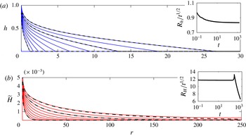
Figure 2 shows snapshots of the height
 $h$
of the interface and of the surface displacement
 $\widetilde{H}=H-1$
. Comparison of these snapshots reveals that
 $h$
and
 $H$
have quite different profiles. In particular, the uplift of the medium spreads far ahead of the location of the injected fluid. As remarked above, the injected current has a sharp front at
 $r=R_{h}(t)$
, where
 $h\rightarrow 0$
with finite slope, with no discernible signature in the profile of the upper surface at that point. By contrast, the upper surface smoothly levels off with no clear nose; that is, it does not have compact support. Indeed, we will show in § 4.1 that the uplift propagates in a linear diffusive manner ahead of the injected current. To measure the radial extent of the uplift,
 $R_{H}(t)$
, we are therefore forced to adopt a nominal threshold amplitude; in figure 2 this is chosen to be
 $10^{-5}$
, so that
 $H(R_{H},t)=10^{-5}$
.
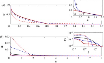
Snapshots from numerical simulations with the default parameter settings given at the start of § 3, with
 $r_{edge}=250$
, at times
 $t=0,2,4,8,16,32,64,128,256,512$
and 1024 (solid), together with the equivalent similarity solutions evaluated at
 $t=2$
,
 $t=256$
and
 $t=1024$
(dashed). (a) The height
 $h(r,t)$
of the injected current and (b) the uplift
 $\widetilde{H}(r,t)=H(r,t)-1$
. Note the different horizontal scales. The insets show the radial extents
 $R_{h}$
and
 $R_{H}$
of the injected current and the uplift, respectively, defined as
 $h(R_{h},t)=0$
and
 $\widetilde{H}(R_{H},t)=10^{-5}$
.

Figure 2 also demonstrates that solutions evolve to self-similar form, with both
 $h(r,t)$
and
 $\widetilde{H}(r,t)$
converging to specific functions of the similarity variable
 ${\it\eta}\equiv r/t^{1/2}$
. The insets in figure 2 show in more detail how the front of the injection spreads self-similarly after a short transient, whereas the (thresholded) radial extent of the uplift adopts the self-similar form immediately, but deviates from this scaling once
 $R_{H}(t)$
reaches the far edge of the domain. Inevitably, this collision leads to a slight deviation from the self-similar form for the profiles of
 $\widetilde{H}$
in the vicinity of the edge of the domain at later times (see comparison of dashed and solid lines in figure 2
b). However, the self-similar form of
 $h(r,t)$
and
 $\widetilde{H}(r,t)$
is still maintained over the bulk of the domain.
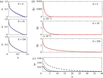
Similarity solutions with
 $M=1$
for different values of the elastic modulus
 $E$
as marked, in terms of the similarity variable
 ${\it\eta}\equiv r/t^{1/2}$
. (a) The height
 $z=h$
of the injected current (solid) with the similarity solution for
 $E\rightarrow \infty$
(dashed; see § 4.2). (b) The uplift
 $\widetilde{H}=H-1$
. (c) The increase in the surface pore pressure
 $\widetilde{P}=P-\mathscr{P}$
, for
 $E=4$
(solid),
 $E=16$
(dotted) and
 $E=256$
(dashed). Note the different scales in the different horizontal scales between (a) and (b), and the different vertical scales in (b).

3.2. Similarity solutions with
 $M=1$

The similarity solutions can be obtained directly by rewriting the governing PDEs (2.35) as a fourth-order system of ODEs, using the transformations
 $\partial /\partial r\rightarrow \partial /\partial {\it\eta}$
and
 $\partial /\partial t\rightarrow (-{\it\eta}/2)\partial /\partial {\it\eta}$
. Alternatively, provided they have converged to self-similar form, similarity solutions can be extracted directly from suitable snapshots of solutions of the PDEs. Here we predominantly use the latter approach, but have verified that it gives the same answer as the former.
Figure 3 shows solutions of the interface height
 $h$
, the uplift
 $\widetilde{H}=H-1$
, and the increase in the pore pressure at the upper surface,
 $\widetilde{P}=P-\mathscr{P}$
, for different values of the elastic modulus
 $E$
. The figure confirms the previous observation that the uplift spreads ahead of the position of the injected fluid, but also shows that
 $h$
and
 $H$
have a quite different dependence on
 $E$
. In particular, while
 $h$
is largely unaffected by changes in
 $E$
(figure 3
a), the radial spread of the uplift increases and its magnitude decreases as the medium becomes stiffer (figure 3
b). Profiles of the surface overpressure
 $\widetilde{P}$
, which is a potentially important variable when considering the possibility of fractures or failures in the medium, mirror those of the uplift (figure 3
c), except near the point in injection where the pressure profiles are rounded off. Unlike the uplift, the magnitude of
 $\widetilde{P}$
increases with the stiffness of the medium.
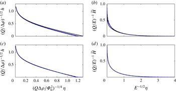
Figure 4 shows solutions of
 $h$
and
 $\widetilde{H}$
for a selection of different parameter values. The results collapse onto roughly the same profiles when the similarity variable
 ${\it\eta}\equiv r/t^{1/2}$
and
 $h$
are scaled by
 $$\begin{eqnarray}{\it\eta}\sim \left(\frac{Q{\rm\Delta}{\it\rho}}{{\it\Phi}_{0}^{2}}\right)^{1/4},\quad h\sim \left(\frac{Q}{{\rm\Delta}{\it\rho}}\right)^{1/2},\end{eqnarray}$$
(figure 4
a,c) and when
 ${\it\eta}$
and
 $\widetilde{H}$
are scaled by
 $$\begin{eqnarray}{\it\eta}\sim E^{1/2},\quad \widetilde{H}\sim \frac{Q}{E},\end{eqnarray}$$
(figure 4 b,d). A theoretical basis for these scalings will be discussed in § 4.
Similarity solutions of (a,c) the scaled interface height and (b,d) the scaled uplift against the scaled similarity variable. (a,b) Comparison for different values of the elastic modulus
 $E$
:
 $E=4$
(black solid),
 $E=16$
(blue solid),
 $E=256$
(black dashed),
 $E=1024$
(blue dashed). (c,d) Comparison for
 $E=256$
and different values of the other parameters:
 $Q=0.1$
,
 ${\it\rho}_{1}=0.7$
,
 ${\it\Phi}_{0}=0.3$
(black solid),
 $Q=0.025$
(blue solid),
 ${\it\rho}_{1}=0.9$
(black dashed),
 ${\it\Phi}_{0}=0.1$
(blue dashed). All unquoted parameters are given by the default values at the start of § 3. The only appreciable deviation from the scalings is for
 $E=4$
in (a,b).

3.3. Similarity solutions with viscosity ratio
$M\neq 1$

There are a number of differences to the dynamics discussed above when
 $M={\it\mu}_{1}/{\it\mu}_{2}\neq 1$
. Figure 5 shows that, for
 $M<1$
(ambient fluid is more viscous than injected fluid), both the height of the injected current and the height of the uplift differ significantly from when
 $M=1$
. The injected current extends further but the height is lower, as has been observed in non-deformable porous layers (Nordbotten & Celia Reference Nordbotten and Celia2006; Pegler, Huppert & Neufeld Reference Pegler, Huppert and Neufeld2014), while the magnitude of the uplift increases. The uplift also becomes more localized to the position of the injected fluid rather than spreading ahead of the current. For
 $M>1$
(figure 5) (ambient fluid is less viscous than injected fluid), the height of the injected current is almost indistinguishable from when
 $M=1$
, although the uplift is enhanced and is more localized when
 $M$
is increased (figure 5
b; inset). The different behaviour of the system for
 $M\neq 1$
is rationalized by the asymptotic analysis of the model in the following section. We find that the behaviour for
 $M>1$
can be explained within the framework of an analysis for general
 $M$
(§§ 4.1 and 4.2), but a quite distinct set of scalings for both the uplift and the current emerge in the limit
 $M\ll E^{-1/2}$
, as discussed in § 4.3. As for a non-deformable medium (see Pegler et al.
Reference Pegler, Huppert and Neufeld2014), this axisymmetric, shallow-layer formulation does not predict Saffman–Taylor fingering for any values of
 $M$
.
Similarity solutions for different values of the viscosity ratio
 $M={\it\mu}_{1}/{\it\mu}_{2}$
:
 $M=0.01$
(red dashed),
 $M=0.1$
(blue dashed),
 $M=1$
(black solid),
 $M=10$
(blue solid) and
 $M=100$
(red solid). (a) The height
 $h$
, with (inset) a comparison for
 $M=0.01$
with the asymptotic results of § 4.3, showing
 $h$
(blue),
 $(H-1)/{\it\Phi}_{0}$
(red) and the solution (black dashed) of the relevant asymptotic evolution equation (4.19b
). (b) The uplift
 $\widetilde{H}$
, with (inset) the same data on logarithmic axes. Note that, in (a), the profiles for
 $M\geqslant 1$
are very similar and the separate lines are difficult to distinguish.

4. Asymptotic limits of the model for large elastic modulus
$E\gg 1$

The numerical solutions indicate that both the uplift and the injected current converge to the same self-similar form in terms of
 ${\it\eta}\equiv r/t^{1/2}$
. However, both the form of the profiles of
 $h$
and
 $H$
and their dependence on the different parameters of the model are quite different. In particular, the uplift propagates far ahead of the injected current, which appears to be almost independent of
 $E$
for
 $E>O(10)$
. In this section we rationalize the different features of the injected current and the uplift by means of an asymptotic analysis of the model for
 $E\gg 1$
. We find that the uplift has a radial scale
 ${\sim}E^{1/2}$
and obeys a linear diffusion equation ahead of the injected fluid (§ 4.1), which itself has an
 $O(1)$
radial extent and a form that reduces to the standard solution for a gravity current in a non-deformable medium (§ 4.2). Interestingly, the separation of radial scales between uplift and injected fluid breaks down if the injected fluid is much less viscous than the ambient fluid, such that
 $M\ll E^{-1/2}\ll 1$
; a new set of scalings emerge in this limit, and both
 $h$
and
 $H$
have a radial scale
 ${\sim}E^{1/4}$
(§ 4.3).
4.1. The uplift
Ahead of the injected current,
 $h=0$
and the hydrostatic pressure and porosity profiles, given from (2.27) and (2.28), are
 $$\begin{eqnarray}p=P+{\it\rho}_{2}(H-z),\end{eqnarray}$$
 $$\begin{eqnarray}{\it\phi}=1-(1-{\it\Phi})\text{e}^{(H-z)\widehat{{\it\rho}}_{2}/E};\quad {\it\Phi}=1-(1-{\it\Phi}_{0})\frac{\text{e}^{\widehat{{\it\rho}}_{2}/E}-1}{\text{e}^{H\widehat{{\it\rho}}_{2}/E}-1},\end{eqnarray}$$
respectively. The evolution equation for the uplift
 $H$
, given from (2.32), is
 $$\begin{eqnarray}\frac{\partial H}{\partial t}=\frac{M}{r}\frac{\partial }{\partial r}\left\{rH\left[{\it\rho}_{2}+\frac{\widehat{{\it\rho}}_{2}(1-{\it\Phi}_{0})[\text{e}^{\widehat{{\it\rho}}_{2}/E}-1]}{[\text{e}^{H\widehat{{\it\rho}}_{2}/E}-1]^{2}}\text{e}^{H\widehat{{\it\rho}}_{2}/E}\right]\frac{\partial H}{\partial r}\right\}.\end{eqnarray}$$
Note that (4.3) is also recovered throughout the domain in the case when the injected fluid is identical to the ambient fluid (
 ${\it\rho}_{1}={\it\rho}_{2}$
and
 ${\it\mu}_{1}={\it\mu}_{2}$
).
For
 $E\gg 1$
, (4.3) reduces to
 $$\begin{eqnarray}\frac{\partial H}{\partial t}=\frac{1}{r}\frac{\partial }{\partial r}\left[\frac{MEr}{H}\frac{\partial H}{\partial r}\right]=\frac{1}{\widetilde{r}}\frac{\partial }{\partial \widetilde{r}}\left[\frac{\widetilde{r}}{H}\frac{\partial H}{\partial \widetilde{r}}\right],\end{eqnarray}$$
in terms of a rescaled radial coordinate
 $\widetilde{r}=r/(ME)^{1/2}$
. This rescaling quantifies the observed scale separation in the numerical solutions: the uplift extends a distance
 ${\sim}(ME)^{1/2}$
ahead of the injected current. On the relatively long radial scale
 $\widetilde{r}$
, the injection appears as a point source of ambient fluid with flux
 $$\begin{eqnarray}\lim _{\widetilde{r}\rightarrow 0}\left[ME\frac{\widetilde{r}}{H}\frac{\partial H}{\partial \widetilde{r}}\right]=-\frac{Q}{2{\rm\pi}}.\end{eqnarray}$$
The source therefore drives a weak uplift
 $H=1+\widetilde{H}$
, with
 $\widetilde{H}=O(Q/(ME))\ll 1$
satisfying the linear diffusion equation
 $$\begin{eqnarray}\frac{\partial \widetilde{H}}{\partial t}=\frac{1}{\widetilde{r}}\frac{\partial }{\partial \widetilde{r}}\left(\widetilde{r}\frac{\partial \widetilde{H}}{\partial \widetilde{r}}\right),\end{eqnarray}$$
from (4.4), which rationalizes the diffusive character of the numerical solutions. Moreover, the self-similar form of the far-field uplift is given from (4.5) and (4.6) by
 $$\begin{eqnarray}H-1=\frac{Q}{ME}\,f\left(\frac{{\it\eta}}{\sqrt{ME}}\right),\end{eqnarray}$$
where
 $f(x)$
satisfies the ODE
 $(xf^{\prime })^{\prime }+x^{2}f^{\prime }/2=0$
. The predictions in (4.7) confirm the observed scalings shown in figure 4 and reported in (3.2), and generalize them for
 $M\neq 1$
and
 $M\gg E^{-1/2}$
(see § 4.3). The separation of length scales between the injected current and the uplift implies that the latter is insensitive to the detailed dynamics of the injected fluid in this limit. Note that the scaling in (4.7b
) is just the classical poro-elastic diffusion scale; see e.g. Coussy (Reference Coussy2004).
4.2. The injected current
For
 $E\gg 1$
and
 $h>0$
, the porosity becomes
 $$\begin{eqnarray}{\it\phi}={\it\Phi}=1-\frac{1-{\it\Phi}_{0}}{H},\end{eqnarray}$$
to leading order, from (2.28) and (2.31), such that
 ${\it\phi}$
is independent of depth. Hence
 $$\begin{eqnarray}\frac{\partial {\it\Phi}}{\partial H}=\frac{1-{\it\Phi}_{0}}{H^{2}},\quad \frac{\partial {\it\Phi}}{\partial h}=-\frac{h(1-{\it\Phi}_{0})^{2}{\rm\Delta}{\it\rho}}{EH^{2}},\end{eqnarray}$$
which can be used to evaluate
 $\partial P/\partial r$
and thus the leading-order fluxes
 $J_{1}$
and
 $J_{2}$
in (2.33):
 $$\begin{eqnarray}\displaystyle & \displaystyle J_{1}=-\frac{E\,h}{H^{2}}\frac{\partial H}{\partial r}-{\rm\Delta}{\it\rho}\left[h-\frac{(1-{\it\Phi}_{0})h^{2}}{H^{2}}\right]\frac{\partial h}{\partial r}, & \displaystyle\end{eqnarray}$$
 $$\begin{eqnarray}\displaystyle & \displaystyle J_{2}=-\frac{E\,M(H-h)}{H^{2}}\frac{\partial H}{\partial r}+\frac{M{\rm\Delta}{\it\rho}(1-{\it\Phi}_{0})h(H-h)}{H^{2}}\frac{\partial h}{\partial r}. & \displaystyle\end{eqnarray}$$
 $J_{1}$
and
 $J_{2}$
must be
 $O(1)$
, which implies that
 $\partial H/\partial r=O(E^{-1})$
in (4.10). Hence, as above,
 $H=1+\widetilde{H}$
with
 $\widetilde{H}=O(E^{-1})\ll 1$
, and so
 $$\begin{eqnarray}\frac{\partial H}{\partial t}=-\frac{1}{r}\frac{\partial }{\partial r}r(J_{1}+J_{2})=O(E^{-1})\ll 1,\end{eqnarray}$$
which indicates that the total flux
 $r(J_{1}+J_{2})$
is a constant to leading order, given by
 $Q/2{\rm\pi}$
. The slope of the uplift becomes
 $$\begin{eqnarray}E\frac{\partial \widetilde{H}}{\partial r}=-{\rm\Delta}{\it\rho}\left[\frac{1}{[h+(1-h)M]}-(1-{\it\Phi}_{0})\right]h\frac{\partial h}{\partial r}-\frac{Q}{2{\rm\pi}r[h+(1-h)M]},\end{eqnarray}$$
to leading order, from (4.11) and (4.10). The terms involving the uplift can thus be eliminated from (4.10a ), and the evolution equation (2.32a ) reduces to
 $$\begin{eqnarray}{\it\Phi}_{0}\frac{\partial h}{\partial t}=\frac{1}{r}\frac{\partial }{\partial r}\left[\frac{-Qh}{2{\rm\pi}[h+(1-h)M]}+{\rm\Delta}{\it\rho}\frac{rh(1-h)M}{h+(1-h)M}\frac{\partial h}{\partial r}\right]+O(E^{-1}),\end{eqnarray}$$
which is the standard evolution equation for the height of a gravity current with a fixed flux
 $Q$
in a confined, non-deformable, porous medium (see, e.g. Pegler et al.
Reference Pegler, Huppert and Neufeld2014). Provided that the injected current does not fill the layer, (4.13) can be approximated by taking the limit
 $h\ll 1$
to give the equation for a gravity current in an unbounded medium (Lyle et al.
Reference Lyle, Huppert, Hallworth, Bickle and Chadwick2005), which yields similarity scalings of
 $$\begin{eqnarray}h\sim \left(\frac{Q}{{\rm\Delta}{\it\rho}}\right)^{1/2},\quad {\it\eta}\equiv r/t^{1/2}\sim \left(\frac{Q{\rm\Delta}{\it\rho}}{{\it\Phi}_{0}^{2}}\right)^{1/4},\end{eqnarray}$$
for the height and extent of the injected current. These scalings were observed in the full similarity solutions in (3.1) and in figure 4. Interestingly, the scalings appear to hold all the way down to
 $E=4$
, which suggests that the influence of the uplift on the injected current is negligible except in very deformable media (small
 $E$
).
A further interesting feature of the leading-order equations (4.8)–(4.10) is that they correspond to the limit of neglecting gravity (i.e. purely pressure-driven flow), because
 $E\propto 1/g$
(cf. (2.15)). However, in this limit we cannot deduce that
 $H$
is constant to leading order, as in (4.11), since time has also been scaled by
 $1/g$
(see § 2.2). Instead, the time derivatives in the evolution equations must be balanced with terms proportional to
 $E$
in (4.10) to give equations for the evolution of
 $h$
and
 $H$
in the absence of gravity:
 $$\begin{eqnarray}\frac{\partial }{\partial \widetilde{t}}({\it\Phi}h)=\frac{1}{r}\frac{\partial }{\partial r}\left[\frac{rh}{H^{2}}\frac{\partial H}{\partial r}\right];\quad \frac{\partial H}{\partial \widetilde{t}}=\frac{1}{r}\frac{\partial }{\partial r}\left[\frac{r[h+(H-h)M]}{H^{2}}\frac{\partial H}{\partial r}\right],\end{eqnarray}$$
where
 $\widetilde{t}=Et$
and
 ${\it\Phi}=1-(1-{\it\Phi}_{0})/H$
from (4.8). The evolution of both injected fluid and uplift are governed by gradients in the slope of the overburden in this limit.
4.3. Small viscosity ratio
$M\equiv {\it\mu}_{1}/{\it\mu}_{2}\ll 1$

The features of the model for
 $E\gg 1$
discussed above change when the viscosity ratio
 $M$
is sufficiently small, such that the ambient fluid is much more viscous than the injected fluid. This is potentially the case for
 $\text{CO}_{2}$
sequestration, where the injected
 $\text{CO}_{2}$
has a much lower viscosity than the ambient brine; we consider this issue in § 6.
The key to understanding the change in behaviour is first to observe that the flux of ambient fluid,
 $J_{2}$
, is proportional to
 $M$
, and so the evolution equations (2.32) can be combined to give
 $$\begin{eqnarray}\frac{\partial }{\partial t}({\it\Phi}h)=\frac{\partial H}{\partial t}-O(M),\end{eqnarray}$$
since the porosity is still given by (4.8) for
 $E\gg 1$
and so is independent of depth. Equation (4.16) implies
 $$\begin{eqnarray}h=\frac{\widetilde{H}}{{\it\Phi}}+O(M).\end{eqnarray}$$
In other words, the height of the injected current is small, and it undercuts the more viscous ambient fluid which is plugging up the porous layer. Moreover, the uplift becomes coupled directly to the injected fluid current and no longer diffuses ahead.
In view of (4.17), the leading-order fluxes
 $J_{1}$
and
 $J_{2}$
in (4.10) simplify still further and the evolution equations (2.32) reduce to
 $$\begin{eqnarray}\frac{\partial }{\partial t}({\it\Phi}h)=\frac{E}{r}\frac{\partial }{\partial r}\left(\frac{rh}{H^{2}}\frac{\partial \widetilde{H}}{\partial r}\right),\quad \frac{\partial \widetilde{H}}{\partial t}=\frac{E}{r}\frac{\partial }{\partial r}\left[\frac{r[h+(H-h)M]}{H^{2}}\frac{\partial \widetilde{H}}{\partial r}\right].\end{eqnarray}$$
To satisfy both (4.17) and (4.18) simultaneously, we can no longer deduce that
 $\widetilde{H}=O(E^{-1})$
as in § 4.2. Instead, provided
 $M\ll h\ll 1$
(which we establish below), we find that (4.17) and (4.18) reduce to
 $$\begin{eqnarray}h=\frac{H-1}{{\it\Phi}};\quad \frac{\partial h}{\partial t}=\frac{E}{r}\frac{\partial }{\partial r}\left(rh\frac{\partial h}{\partial r}\right),\end{eqnarray}$$
and a change in the scaling of the radial structure of the solution is required. In particular, (4.19) (which has the same form as a standard equation for a gravity current in a porous medium) together with the boundary condition
 $-Q/2{\rm\pi}={\it\Phi}_{0}Erh(\partial h/\partial r)$
as
 $r\rightarrow 0$
, furnish the similarity solution,
 $$\begin{eqnarray}h=\frac{H-1}{{\it\Phi}_{0}}=\left(\frac{Q}{{\it\Phi}_{0}E}\right)^{1/2}f\left(\frac{{\it\eta}}{(QE/{\it\Phi}_{0})^{1/4}}\right),\end{eqnarray}$$
where
 $f(x)$
satisfies the ODE
 $(xff^{\prime })^{\prime }+x^{2}f/2=0$
. Thus, the height of the current and uplift are indeed small:
 $h\sim \widetilde{H}\sim O(E^{-1/2})$
. The condition
 $M\ll h$
demands that
 $M\ll E^{-1/2}\ll 1$
, which identifies the viscosity ratio for which the scalings change. If either
 $M>O(E^{-1/2})$
or
 $h\ll M$
, then (4.18b
) reduces to the linear diffusion equation (4.6) discussed in § 4.1, and the uplift again diffuses ahead of the current.
The scalings in (4.20) can be compared with the previously identified scalings in (4.7) and (4.14). There is a transition from the injected current being driven by buoyancy forces and evolving independently of
 $E$
for
 $M=O(1)$
, scaling as in (4.14), to the current being independent of buoyancy and being controlled by
 $E$
as
 $M\rightarrow 0$
, with scaling (4.20a,b
). The magnitude of the uplift also becomes independent of
 $M$
to leading order. These asymptotic results are consistent with the trends in the numerical results of figure 5; in particular, figure 5(a; inset) shows a relatively good agreement between direct measurement of
 $h$
and the predictions of
 $h$
using either (4.19a
) or solutions to (4.19b
).
5. Laboratory experiments
5.1. Experimental results
To complement the theory, we carried out laboratory experiments using polyacrylamide hydrogel particles. Dry particles swell to roughly 40 times their size on the addition of water, and form soft, elastic, roughly spherical beads of radius
 $0.38\pm 0.08~\text{mm}$
. We filled the base of a cylindrical tank, of radius of 445 mm, to a depth of
 $H_{0}=35~\text{mm}$
with a layer of hydrogel particles to form a deformable porous medium (figure 6
a). Because the particles consist predominantly of water, their density is only very slightly higher than
 $1~\text{g}~\text{cm}^{-3}$
. The saturated bed of particles was overlain by a flexible but impermeable polydimethylsiloxane (PDMS) sheet of thickness 5 mm. The sheet fitted closely inside the tank, such that water did not leak around the edges during an experiment. There was a small hole at the base in the centre of the tank through which water could be injected at a fixed flux (using a peristaltic pump) or allowed to drain. Interstitial air in the medium was removed by first significantly over-saturating the particles to produce a thin slurry, before slowly draining excess water to produce a medium that was fully saturated.
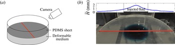
(a) A schematic of the experimental set-up. (b) An image from an experiment in which the injected water was dyed blue to distinguish it from the clear ambient water. The profile above shows the uplift of the upper surface, as measured by the deflection of the line on the PDMS sheet, and demonstrates that the uplift travels ahead of the blue fluid. The flux was
 $Q=100~\text{cm}^{3}~\text{min}^{-1}$
and the image was taken roughly 2 min after the start of injection.

The experiments were intended to provide a relatively simple qualitative comparison with the theoretical model in the limit that the injected and ambient fluid are identical. One-dimensional compression tests suggested that the saturated medium had an elastic modulus of
 $K+4G/3\approx 20{-}30~\text{kPa}$
, in rough agreement with previously quoted values for this material (MacMinn et al.
Reference MacMinn, Dufresne and Wettlaufer2015). The dimensionless stiffness therefore lay in the range
 $70\lesssim E\lesssim 80$
, and so was fairly large, as in the limit considered in our analysis. Despite this, there are a number of complications associated with this experimental set-up which render a systematic comparison with the theoretical model difficult (see § 5.2).
The main variable that was changed between experiments was the injection rate. We also carried out sets of experiments for different depths
 $H_{0}$
of the medium, which are not presented but exhibited qualitatively similar results to those discussed here. During each experiment, we took measurements of the uplift by using a camera to track a line drawn on the surface of the PDMS sheet. The camera was located 770 mm from the centre of sheet at an angle of
 $35^{\circ }$
from the horizontal. Figure 6(b) shows a picture from an experiment in which the injected fluid was dyed blue, together with the measured profile of the uplift of the upper surface. Note that the injected fluid noticeably lags behind the measured uplift.
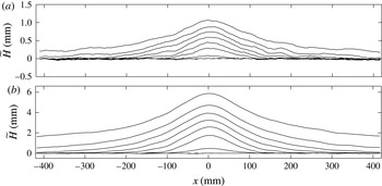
Figure 7 shows measurements of the height of the upper surface over time, for two different injection rates
 $Q$
. The uplift is qualitatively similar to the numerical solutions (see, for example, figure 3
b), except near to the point of injection, where the profiles are smoother. This difference is most likely due to bending stresses in the PDMS sheet, which we estimate to be important on length scales of a few centimetres (see § 5.2). Such stresses eliminate the logarithmic divergence of the uplift
 $\widetilde{H}$
for
 $r\rightarrow 0$
predicted by the model (see appendix A) by rounding off the profile there.
Experimental measurements of the height
 $\widetilde{H}$
of the deviation of the upper surface, in mm, at times
 $t=2,4,8,16,32,64,128$
and 256 s. (a) Injection rate
 $Q=25~\text{cm}^{3}~\text{min}^{-1}$
. (b)
 $Q=200~\text{cm}^{3}~\text{min}^{-1}$
. The coordinate
 $x$
measures the radial distance from the point of injection, such that
 $r=|x|$
.

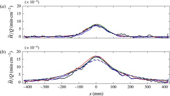
Comparison of figure 7(a,b) suggests that the main difference between the measurements at different injection rates is the magnitude of the uplift, and that the rate at which the uplift propagates radially is largely independent of the flux. This observation is corroborated by snapshots of the uplift for a range of different values of the flux (figure 8), which shows that the profiles collapse onto roughly the same curve when scaled by the injection rate
 $Q$
, in agreement with the theoretical prediction in (4.7a
).
Experimental measurements of the height
 $\widetilde{H}$
of the deviation of the top surface scaled by the injection rate
 $Q$
, at times (a)
 $t=10~\text{s}$
and (b)
 $t=100$
s, for different injection rates
 $Q=25~\text{cm}^{3}~\text{min}^{-1}$
(black solid),
 $Q=50~\text{cm}^{3}~\text{min}^{-1}$
(blue solid),
 $Q=100~\text{cm}^{3}~\text{min}^{-1}$
(red solid),
 $Q=200~\text{cm}^{3}~\text{min}^{-1}$
(green solid),
 $Q=300~\text{cm}^{3}~\text{min}^{-1}$
(black dashed) and
 $Q=400~\text{cm}^{3}~\text{min}^{-1}$
(blue dashed). The coordinate
 $x$
measures the radial distance from the point of injection, such that
 $r=|x|$
. The noise in the profiles with the lowest injection rates reflects the sub-pixel resolution of the processed images (achieved using a Gaussian fit to the intensity of the tracked line), which was roughly
 $50~{\rm\mu}\text{m}$
.

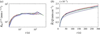
Given that the uplift scales with the injection rate, we identify the radial extent of the uplift by choosing a threshold in
 $\widetilde{H}/Q$
. More specifically, we define
 $$\begin{eqnarray}R_{H}=\min \{r:\,\widetilde{H}<2Q\times 10^{-3}\}.\end{eqnarray}$$
Measurements of
 $R_{H}$
from the experiments (figure 9) agree qualitatively with the predicted scalings in (4.7), with the radial spread being largely independent of the injection rate
 $Q$
and scaling with
 $t^{1/2}$
until
 $R_{H}$
reaches the edge of the tank. The spread also slightly accelerates close to the boundary of the tank, as observed in the numerical solutions in a finite domain (figure 2
b inset). Contrary to theory, the uplift spreads initially (up to
 ${\sim}10~\text{s}$
) more rapidly than
 $t^{1/2}$
and the height above the point of injection increases steadily. The disagreement with theory is again most likely due to bending stresses in the overburden near the origin, at least at early times. At later times, the pressure signal has reached the edge of the domain and the entire overburden is lifting up.
Experimental measurements for different injection rates:
 $Q=25~\text{cm}^{3}~\text{min}^{-1}$
(black solid),
 $Q=50~\text{cm}^{3}~\text{min}^{-1}$
(blue solid),
 $Q=100~\text{cm}^{3}~\text{min}^{-1}$
(red solid),
 $Q=200~\text{cm}^{3}~\text{min}^{-1}$
(green solid),
 $Q=300~\text{cm}^{3}~\text{min}^{-1}$
(black dashed) and
 $Q=400~\text{cm}^{3}~\text{min}^{-1}$
(blue dashed). (a) The radial extent
 $R_{H}$
, defined by (5.1), of the uplift, scaled by
 $t^{1/2}$
. The measurements are approximately independent of
 $Q$
and show a scaling of
 $t^{1/2}$
until
 $R_{H}$
reaches the edge of the tank. (b) The height
 $\widetilde{H}(r=0)$
above the point of injection, scaled by
 $Q$
.

5.2. Limitations of the experiments
The experimental system provides a simple laboratory-scale deformable porous medium, with which we have been able to confirm qualitatively some of the theoretical results. There are some difficulties in using hydrogel particles as an idealized poro-elastic medium, which prevented a more quantitative comparison with the model. In particular, the particles are always coated with a layer of water, and it is not clear whether their aqueous contents continually leak out. In this situation it is very difficult to distinguish the effective solid phase from the fluid, and therefore to measure the initial porosity. We also found that the elastic modulus of the saturated medium varies appreciably with the porosity, which complicates the characterization of the properties of the medium.
One of the notable features of the experimental results is the influence of bending in the overburden around the point of injection. The flexural rigidity
 $B$
of the PDMS sheet was
 $B\approx 0.024~\text{Pa}~\text{m}^{3}$
(given a Young’s modulus of
 ${\approx}1.8~\text{MPa}$
, a thickness of 5 mm and a Poisson ratio of 0.45; see Lister, Peng & Neufeld, Reference Lister, Peng and Neufeld2013). The relative importance of bending in the balance of stresses (2.23) at the upper surface is given by the ratio of the bending pressure
 $B{\rm\nabla}^{4}H$
to the hydrostatic pressure
 ${\it\rho}gH$
. Such a balance gives a rough length scale of
 $r\approx 4~\text{cm}$
over which bending is likely to affect the uplift, which is consistent with the length scale of the rounding of the profiles around the point of injection in figures 7 and 8. A similar analysis can be carried out in a geophysical context: for an overburden rock with Young’s modulus 10 GPa and depth 1 km, bending of the overburden would affect the uplift for roughly 1 km around the injection site.
6. Conclusions
In this paper, we used a two-phase poro-elastic formulation and shallow-layer scalings to describe the injection and gravity-driven spread of fluid in an axisymmetric poro-elastic layer lying on a rigid horizontal substrate and below a flexible overburden. We derived a model coupling the evolution of the height
 $h(r,t)$
of the injected current with the resultant deformation of the medium and corresponding uplift
 $H(r,t)$
of the overburden. In the absence of an external radial length scale, both
 $h$
and
 $H$
are described by self-similar solutions with respect to the similarity variable
 ${\it\eta}\equiv r/t^{1/2}$
. In geophysical settings, the dimensionless modulus or stiffness
 $E$
, which is the ratio of elastic to gravitational stresses, is typically large, and we focused on that limit in this work.
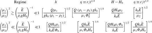
We found that deformation of the medium has, in general, only a very small effect on the dynamics of the injected fluid. In many geological cases, the current evolves as a standard gravity current in a rigid porous medium (see the scalings in table 1), and is largely independent of the stiffness for moderate to large
 $E$
, provided the viscosity of the ambient fluid
 ${\it\mu}_{2}$
is not much larger than that of the injected fluid
 ${\it\mu}_{1}$
(specifically,
 ${\it\mu}_{1}/{\it\mu}_{2}>O(E^{-1/2})$
). The uplift of the medium, on the other hand, varies significantly with the stiffness. There is a separation of radial scales between the uplift and the injected fluid: the uplift spreads in a linear diffusive manner ahead of the injected fluid and is insensitive to the detailed dynamics of the spreading current (see table 1).
A summary of the dimensional scalings of the heights
 $z=h$
and
 $z=H$
and of the corresponding similarity variables
 ${\it\eta}\equiv r/t^{1/2}$
for injection with a constant (dimensional) flux
 $Q$
, where
 $H_{0}$
is the depth of the layer,
 $g$
is the gravitational acceleration,
 ${\it\rho}_{1}$
,
 ${\it\rho}_{2}$
and
 ${\it\rho}_{s}$
are the densities of the injected and ambient fluids and of the solid phase,
 ${\it\mu}_{1}$
and
 ${\it\mu}_{2}$
are the viscosities of the injected and ambient fluids,
 ${\it\Phi}_{0}$
and
 $k_{0}$
are characteristic porosity and permeability scales (all respectively), and
 $\widetilde{E}\equiv K+4G/3$
combines the bulk modulus
 $K$
and shear modulus
 $G$
of the porous medium. Note that the scalings presented for
 $h$
and
 ${\it\eta}$
in the top line are the scalings for a porous gravity current in a deep domain (Lyle et al.
Reference Lyle, Huppert, Hallworth, Bickle and Chadwick2005), which will apply for as long as the injection does not fill up the porous layer; see Pegler et al. (Reference Pegler, Huppert and Neufeld2014). The scaling of
 ${\it\eta}$
for the uplift in the top line is the classical poro-elastic diffusion scale (Coussy Reference Coussy2004).

Owing to this diffusive character, there is no true front to the outgoing signal of the uplift. Instead, its radial spread
 $r_{H}(\mathscr{H})$
must be defined using a prescribed threshold
 $H-H_{0}=\mathscr{H}$
in the elevation change. In fact, because the full diffusion solution of (4.7) has a Gaussian nose, it can be shown that
 $$\begin{eqnarray}r_{H}\sim \left(\frac{k_{0}\widetilde{E}}{{\it\mu}_{2}}\right)^{1/2}\left[\log \left(\frac{Q{\it\mu}_{2}}{\mathscr{H}k_{0}\widetilde{E}}\right)\right]^{1/2}t^{1/2},\end{eqnarray}$$
where the dependence on viscosity
 ${\it\mu}_{2}$
, elastic modulus
 $\widetilde{E}\equiv (K+4G/3)$
, injection rate
 $Q$
and permeability scale
 $k_{0}$
follow from the detailed similarity solution of (4.7). The radial extent
 $r_{H}$
of the uplift is therefore only weakly dependent on the rate of injection
 $Q$
, and is independent of the buoyancy terms, the initial porosity
 ${\it\Phi}_{0}$
, and the viscosity of injected fluid
 ${\it\mu}_{1}$
, all of which affect the evolution of the injected current.
Both the uplift and the height of the injected fluid are functions of the same similarity variable, and the ratio
 $r_{h}/r_{H}$
of the radial spread of injected fluid to that of the uplift is therefore independent of time. Using (6.1) and the scalings in table 1, we estimate
 $$\begin{eqnarray}\frac{r_{h}}{r_{H}}\sim \left[\frac{Q({\it\rho}_{1}-{\it\rho}_{2})g{\it\mu}_{2}^{2}}{k_{0}\widetilde{E}^{2}{\it\Phi}_{0}^{2}{\it\mu}_{1}}\right]^{1/4}\left[\log \left(\frac{Q{\it\mu}_{2}}{\mathscr{H}k_{0}\widetilde{E}}\right)\right]^{-1/2}.\end{eqnarray}$$
If an uplift of
 $\mathscr{H}$
is observed at a radial distance
 $r_{\mathscr{H}}$
, this ratio allows one to determine the predicted extent
 $r_{h}$
of the injected fluid.
In many physical situations, the pore pressure, rather than the flux, is imposed at the point of injection. In the appendix A, we studied injection with a fixed pore pressure, and found that the dynamics of constant-pressure injections evolve to be essentially equivalent to those for constant flux. This conclusion applies for as long as a significant pressure signal has not reached a far boundary of the domain, which is also when our constant-flux solutions deviate from self-similar behaviour.
In contrast to this behaviour, in an idealized non-deformable medium the dynamics associated with injection at a fixed pressure must inevitably depend upon the far-field boundary conditions because of the pressure gradients that are immediately set-up. In a deformable medium the pressure signal spreads diffusively and the nearest boundary at
 $r=r_{edge}$
will have a negligible effect on the dynamics until significant pressure has built up there, which occurs over a time scale of
 $t\sim {\it\mu}_{2}r_{edge}^{2}/k_{0}\widetilde{E}$
. Example parameter values from In Salah (Rutqvist et al.
Reference Rutqvist, Vasco and Myer2010) suggest times of the order of
 $10^{3}$
days if the nearest boundary or obstacle is at
 $r_{edge}=10~\text{km}$
. Until this time, the dynamics will evolve essentially independently of any far-field conditions, such as faults or fractures in the medium.
Interestingly, if the injected fluid is much less viscous than the ambient fluid (so that
 ${\it\mu}_{1}/{\it\mu}_{2}\ll E^{-1/2}$
), then the conclusions discussed above break down. In this case (discussed in § 4.3), the injected fluid undercuts the much more viscous ambient fluid which plugs up the medium. The uplift then becomes localized to the position of the injected current rather than diffusing ahead, and the dependence on the parameters change (see table 1). In the context of
 $\text{CO}_{2}$
sequestration, however, we estimate that
 $E>O(10^{3})$
while
 ${\it\mu}_{1}/{\it\mu}_{2}\approx 1/20$
. Thus, although the viscosity ratio is small, it is unlikely to be smaller than
 $E^{-1/2}$
.
In this work we have focused on relatively large values of the stiffness
 $E$
, since this is the limit appropriate to geophysical contexts. An interesting extension of the model is to consider situations with significant deformation, as in some biological applications. A first step in this direction requires the relaxation of linear poro-elasticity. In such a situation it may also prove necessary to remove the assumption that the fluid and solid phases move together as the overburden lifts up. A pocket of fluid may then float up above the solid matrix to lubricate the overburden, or fluid may drain away underneath as the solid lifts up.
Acknowledgements
D.R.H. is grateful for funding from the PANACEA project and the Killam Foundation. J.A.N. is supported by a Royal Society University Research Fellowship.
Appendix A. Fixed pore pressure at the point of injection
Fluid may be injected at a fixed pore pressure, rather than a fixed flux. In this appendix, we consider injection at a fixed pressure
 $p_{I}$
and show that the flow is qualitatively similar to that with a (related) fixed flux
 $Q$
, until significant uplift has reached a boundary of the domain. As we will show below, infinite pore pressure is required at
 $r=0$
to sustain a non-zero flux, which implies that we must consider a finite fixed pressure
 $p_{I}$
at a small non-zero radius of injection
 $r_{I}$
. In this case, the boundary condition of fixed flux (2.24a
) is replaced by
 $$\begin{eqnarray}p(r=r_{I},z=0)=p_{I},\end{eqnarray}$$
or, equivalently, using the expression for hydrostatic pressure (2.27) and the balance of normal stress at
 $z=H$
(2.29),
 $$\begin{eqnarray}\widetilde{p}_{I}-{\it\rho}_{2}(H-h)-{\it\rho}_{1}h=E\frac{{\it\Phi}-{\it\Phi}_{0}}{1-{\it\Phi}_{0}},\quad \text{at }r=r_{I},\end{eqnarray}$$
where
 $\widetilde{p}_{I}=p_{I}-\mathscr{P}$
is the excess imposed pore pressure above the overburden pressure. Equation (A 2) can be combined with the equation for
 ${\it\Phi}(h,H)$
(2.31) to give an implicit relationship between
 $H$
and
 $h$
at
 $r=r_{I}$
, which can be solved iteratively together with the constraint that there is no flux of ambient fluid at
 $r=r_{I}$
(2.34b
). The corresponding flux
 $Q(t)$
is given by (2.34a
).
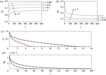
Figure 10 compares results from numerical simulations with fixed flux and fixed pressure at
 $r=r_{I}$
. After an initial transient, simulations with fixed flux have an almost constant pressure
 $\widetilde{p}_{I}$
(figure 10
a), while simulations with fixed pressure have an almost constant flux
 $Q$
(figure 10
b). Figure 10(c,d) emphasizes the correspondence by comparing solutions in which the near-constant flux of the constant-pressure injection was matched by that of an injection with constant flux. In common with most other porous or viscous gravity-current problems, the profiles for fixed flux and non-zero
 $r_{I}$
also give very good agreement with the similarity solution.
Comparison of profiles from simulations with fixed flux
 $Q$
or fixed pressure
 $\widetilde{p}_{I}$
at
 $r=r_{I}$
. (a) The pressure
 $\widetilde{p}_{I}$
at
 $r_{I}$
from simulations with fixed flux
 $Q=0.1$
, for different
 $r_{I}=1$
as marked. (b) The flux
 $Q$
at
 $r_{I}$
from simulations with fixed pressure
 $\widetilde{p}_{I}=0.72$
, for different
 $r_{I}=1$
as marked. (c,d) The height
 $h(r,t)$
of the injected current and the uplift
 $\widetilde{H}(r,t)$
, as marked, at times
 $t=40$
(leftmost group of curves) and
 $t=400$
(rightmost group of curves), with
 $r_{I}=0.1$
, for fixed flux
 $Q=0.1$
(solid) and fixed pressure
 $\widetilde{p}_{I}=0.72$
(short dashed). The simulations with fixed flux agree with the similarity solution (long dashed). The other parameters in these simulations are those given at the start of § 3.

The dynamics of injection with a fixed pressure can be exposed by an analysis of the equations in the limit
 $r_{I}\rightarrow 0$
. Provided that the flux of injected fluid remains non-zero in this limit, we require
 $J_{1}\neq 0$
and
 $J_{2}=0$
from the flux boundary conditions (2.34). These constraints indicate that
 $h\sim H$
as
 $r\rightarrow 0$
; in other words, as
 $r_{I}\rightarrow 0$
the entire layer fills up with injected fluid in some small region close to
 $r=0$
. The shape of
 $h\sim H$
close to
 $r=0$
can be determined from the equation for the flux (2.33a
), which reduces to
 $$\begin{eqnarray}-rh\left({\it\rho}_{1}+\frac{E}{1-{\it\Phi}_{0}}\frac{\partial {\it\Phi}}{\partial h}\right)\frac{\partial h}{\partial r}\rightarrow \frac{Q}{2{\rm\pi}}\quad \text{as }r\rightarrow 0,\end{eqnarray}$$
or
 $$\begin{eqnarray}h\sim H\sim \left[\frac{Q}{{\rm\pi}{\it\rho}_{1}}\log \left(\frac{1}{r}\right)\right]^{1/2}\quad \text{as }r\rightarrow 0.\end{eqnarray}$$
That is, in some exponentially small region near to
 $r=0$
,
 $h\sim H$
diverges. (In the limit
 $h\rightarrow H\rightarrow \infty$
, the gradient of
 ${\it\Phi}$
vanishes and
 ${\it\Phi}\rightarrow 1$
.) The logarithmic divergence of
 $h$
as
 $r\rightarrow 0$
is a generic feature of axisymmetric viscous gravity currents.
The excess pressure
 $\widetilde{p}_{I}$
at
 $r_{I}$
is given by (A 2) which, using (A 4) and
 ${\it\Phi}\rightarrow 1$
, gives
 $$\begin{eqnarray}\widetilde{p}_{I}\sim \left[\frac{{\it\rho}_{1}Q}{{\rm\pi}}\log \left(\frac{1}{r_{I}}\right)\right]^{1/2}+E\quad \text{as }r_{I}\rightarrow 0.\end{eqnarray}$$
In other words, for sufficiently small values of
 $r_{I}$
, the flux and the pressure are directly linked via (A 5), and so flow with a fixed pressure should be the same as flow with the corresponding fixed flux given by (A 5). Equation (A 5) also confirms that the pressure associated with a non-zero flux
 $Q$
diverges as
 $r_{I}\rightarrow 0$
.
The agreement of simulations with fixed flux and fixed pressure in figure 10 is not exact, which does not contradict (A 5) because the radius of injection is not exponentially small in those simulations. For the parameter values of those simulations and
 $h=O(1)$
, (A 4) gives estimates of
 $r_{I}$
of the order of
 $r_{I}\sim \text{e}^{-20}$
, which is many orders of magnitude smaller than can be readily attained numerically.
In a finite domain, we expect a qualitative difference between the dynamics with a fixed-flux and fixed-pressure boundary conditions once significant uplift has reached the far boundary at
 $r=r_{edge}$
. If the pressure were fixed then the flux would decrease significantly, whereas if the flux were fixed then the whole system would became pressurized. The diffusive scalings in (4.7) indicate that this change in the dynamics occurs after a (dimensionless) time scale
 $t\sim r_{edge}^{2}/(ME)$
.