1. Introduction
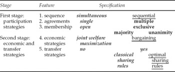
For a long time, the classical approach to study participation in self-enforcing international environmental agreements (IEAs) was based either on the concept of the core (e.g. Chander and Tulkens, Reference Chander and Tulkens1997), belonging to cooperative game theory or on the concept of internal and external stability (e.g. Carraro and Siniscalco, Reference Carraro and Siniscalco1993) belonging to non-cooperative game theory (see Finus, Reference Finus, Folmer and Tietenberg2003, for an overview). Non-cooperative game theory models coalition formation as a two-stage game where players (e.g. countries) decide upon their participation in the first stage and choose their economic strategies (e.g. abatement levels) and possible transfers in the second stage (see table 1). Typically, the game is solved by backward induction.
The structure of coalition formation*

Note: *Standard assumptions are indicated in italics, assumptions considered in this paper are indicated in bold, and assumptions that are proposed for future research are underlined.
In the second stage, the standard assumption is that players belonging to the same coalition choose their economic strategies such as maximizing the aggregate payoff to their coalition (i.e. joint welfare maximization). In the case of heterogeneous players, sharing rules such as Nash bargaining and Shapley value (Botteon and Carraro, Reference Botteon, Carraro and Carraro1997), or the Chander–Tulkens transfer scheme (Barrett, Reference Barrett2001) have been applied. A particular set of assumptions assigns a vector of payoffs to each coalition structure, called valuations. In the first stage, the decision about participation is modeled as a membership game. The standard assumption is a cartel formation game in which players simultaneously announce their decision to remain a singleton or to join the coalition (i.e. cartel). This assumption implies that players can only form a single agreement. The standard definition of stability requires that in equilibrium no player has an incentive to change its announcement. Hence, this concept defines stability in terms of single deviations and implies open membership since players can freely join a coalition.
Recently, there have been advances in non-cooperative coalition theory that are gradually being adopted in the game theoretical analysis of IEAs (e.g. Carraro, Reference Carraro and Siebert2000; Finus and Rundshagen, Reference Finus, Rundshagen and Carraro2003). Until now, these modifications apply exclusively to the first stage of coalition formation (see table 1) and the definition of stable coalitions (not displayed in table 1) as explained for instance in Finus (Reference Finus, Folmer and Tietenberg2003). Those modifications include for instance that stability may be defined not only in terms of single but also multiple deviations (e.g. strong Nash equilibrium or coalition-proof Nash equilibrium). Moreover, the timing of participation decisions may be modeled sequentially, the possibility of multiple coalitions can be considered, as can be various forms of exclusive membership.
In this paper, we focus on the issues of ‘single versus multiple coalitions’ and ‘open versus exclusive membership’. From the theoretical oriented literature, there is some indication that the formation of multiple coalitions and the restriction of membership can enhance the success of self-enforcing IEAs. However, this evidence is based on the assumption of symmetric players and other restrictive assumptions about the payoff functions (e.g. Carraro and Marchiori, Reference Carraro, Marchiori and Carraro2003; Finus and Rundshagen, Reference Finus, Rundshagen and Carraro2003). In this paper, we analyze these issues with an empirical model that comprises benefit and cost estimates for 12 heterogeneous world regions in the context of global warming.Footnote 1 This makes it interesting to analyze whether and how transfers affect coalition formation.
In the following, we describe our model in section 2 and report our results in section 3. In section 4, we place our conclusions in a wider perspective and suggest issues for future research. This includes a discussion of all assumptions listed in table 1 which are not treated in this paper.
2. The model
2.1 First stage of coalition formation
There are several ways to model the notion of single versus multiple coalitions and open versus exclusive membership. We use a notion proposed by Carraro (Reference Carraro and Siebert2000), which emerges as a natural extension of the well-known concept of internal and external stability in the cartel formation game. In the following, we describe this notion informally and provide a formal definition in our working paper (Finus et al., Reference Finus, Sáiz and Hendrix2004).
The notion of single versus multiple coalitions is modeled using two alternative coalition games that both assume that all players {1,. . ., n}, which are world regions in our model and henceforth referred to as regions, simultaneously announce their membership. In the single coalition game, regions have only two membership strategies, called announcements. Announcement σi = 0 implies that the region remains a singleton and announcement σi = 1 implies that the region becomes a member of a non-trivial coalition, provided there is at least one more region that makes the same announcement. In the multiple coalition game, regions have n possible announcements. If a region makes an announcement that no other region makes, this region remains a singleton. Regions that have made the same announcement form a coalition. Consequently, in both games, announcements lead to a coalition structure p = {κ1, κ2, . . ., κM}, which is a partition of players in disjoint sets. In the single coalition game, κ2, . . ., κM are singleton or trivial coalitions, whereas in the multiple coalition game, some or all coalitions κ2, . . ., κM may be non-trivial coalitions.
The notion of open versus exclusive membership is captured by applying different definitions of stability. In the single coalition game, open membership is captured by the (standard) definition of internal and external stability. A coalition structure p = {κ1, {i}, . . ., {k}} that is derived from a set of announcements σ* is stable if no region that announced σi* = 1 has an incentive to change its announcement to σ′i = 0 (internal stability) and if no region that has announced σj* = 0 has an incentive to change its announcement to σ′j = 1 (external stability). In order to capture exclusive membership, we extend the definition of external stability under exclusive membership. In case a region that announced σj* = 0 has an incentive to switch to σj* = 1, we assume that current members of coalition κ1 vote on the accession of this region. We consider two versions: majority and unanimity voting. Majority voting means that accession is only possible if a (strict) majority of current members of coalition κ1 is in favor of accession (i.e. they receive a higher payoff in the enlarged coalition). Under unanimity voting, accession is only possible if all current members of κ1 support the accession of a new member.
In the multiple coalition game, a coalition structure p = {κ1, κ2, . . ., κM} is not only stable if the conditions for internal and external stability are satisfied, but the conditions for intercoalitional stability must also hold. That is, under open membership we also have to ensure that no coalition member has an incentive to join another coalition. Exclusive membership under majority and unanimity voting is captured in a similar way as described for the single coalition game. That is, the definitions of exclusive and intercoalitional stability are modified to account for the fact that if a region has an incentive to join a coalition, current members vote upon its accession.
There are two features that are important to note for the subsequent analysis. Firstly, a coalition structure that is stable under open membership will also be stable under exclusive membership (but not necessarily vice versa) and a coalition structure that is stable under majority voting will also be stable under unanimity voting (but not necessarily vice versa). This is an immediate implication of the definitions of stability. The interesting question is what ‘more stability’ means in terms of global abatement and global welfare. Secondly, on the one hand, the possibility to form multiple coalitions implies more flexibility for regions which might enhance the success of coalition formation. For instance, a region that is not interested in cooperation with the main coalition, as long as this means take it or leave it, may consider forming another coalition with regions that have similar interests. This may mean that this additional coalition implements lower abatement targets but, nevertheless, its members increase abatement above non-cooperative levels. On the other hand, however, more flexibility means also more possibilities to free-ride. For instance, a coalition member that is faced with the option to stay or to quit may decide to remain in the coalition. However, having also the possibility to join another coalition may be an attractive option, jeopardizing stability. Thus, the interesting question is which of the two opposed effects is dominating.
In the context of symmetric players, it has been shown that if coalition formation is not restricted to a single coalition, multiple coalitions will emerge in equilibrium. Moreover, there is some indication that equilibrium coalition structures in the multiple coalition game are superior in terms of global abatement and global welfare than those in the single coalition game. A similar positive impact applies also to exclusive membership (Carraro, Reference Carraro and Siebert2000; Carraro and Marchiori, Reference Carraro, Marchiori and Carraro2003; Finus and Rundshagen, Reference Finus, Rundshagen and Carraro2003). Hence, it remains to be analyzed whether this also holds for heterogeneous players for which we use our empirical model, as sensible analytical results are difficult to obtain.
2.2 The second stage of coalition formation
Basic structure
We assume that the payoff function of region i is given by
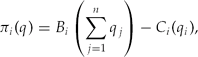
where  represents the benefits from global abatement (which is the sum of individual abatement, q j, ∀ j ∈ I = {1, . . ., n}) and C i(q i) are abatement costs from individual abatement qi, and q is the vector of abatement levels. The strategy space is compact,
 , where e BAUi are business-as-usual emissions in the absence of any abatement. The benefit function is a continuous and concave function and the cost function is a continuous and strictly convex function. Each coalition κl is assumed to choose abatement such as maximizing the sum of payoffs of its individual membersFootnote 2
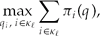
given abatement qj of all players j ∉ κℓ. The simultaneous solution of (2) for all coalitions κℓ in a given coalition structure p = {κ1, κ2, . . ., κM}, yields the (unique) equilibrium abatement vector q*(p). This abatement vector can be interpreted as a Nash equilibrium between coalitions. Within a coalition, the abatement vector is optimal from a cost–benefit perspective of the coalition members. Consequently, the coalition structure where all regions are in one coalition (grand coalition), representing full cooperation, corresponds to the global optimum. By the same token, the coalition structure that comprises only singleton coalitions, representing no cooperation, corresponds to the Nash equilibrium. Any other coalition structure may be seen as partial cooperation.
In the case of no transfers, substituting q*(p) into (1) yields a vector of payoffs π(q*(p)) = (π1(q*(p)),. . ., πN(q*(p))) called valuations, i.e. v(p) = π(q*(p)). In the case of transfers, it is assumed that valuations may be modified through a transfer scheme such that

where t i > 0 means to receive a transfer and t i < 0 means to pay a transfer. In addition, transfers are only paid among coalition members, these transfers balance, i.e.  , and hence
 holds.Footnote 3 We assume transfers of the following form

where pN denotes the coalition structure comprising only singleton coalitions, corresponding to the Nash equilibrium and p ∈ P denotes an arbitrary coalition structure in the set of all coalition structures P. On the right-hand side of the equality, the first two terms set every coalition member back to its non-cooperative payoff that may be regarded as the status quo before coalitions are formed. The third term allocates to each member a portion of the gains from cooperation  , measured as the difference between the aggregate payoff of coalition κl in coalition structure p and the status quo coalition structure pN. Inserting (4) in (3) gives
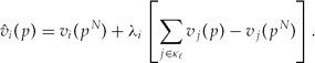
Equation (5) can be interpreted as a Nash bargaining solution with threat points v i(pN) and weights λi, which allocates the collective gain of the coalition κl over no cooperation, which is the term in brackets. In the game theoretical literature, weights are typically interpreted as a reflection of bargaining power (Binmore et al., Reference Binmore, Rubinstein and Wolinsky1986), whereas in the environmental economics literature (Rose and Stevens, Reference Rose and Stevens1998; Rose et al., Reference Rose and Stevens1998) they are typically associated with various notions of equity or fairness as described below. For our analysis, the interpretation of weights is not important as they are exogenous. In our discussion of policy issues, we restrict attention to the dimension of equity and fairness, though it could also be related to bargaining power.
Calibration of the payoff functions
The calibration of payoff function (1) is based on the stability of coalitions (STACO) model. Since the model has been laid out in much detail in Dellink et al. (Reference Dellink2004), and frequently used for instance in Weikard et al. (Reference Weikard, Finus and Altamirano-Cabrera2006), we only briefly describe the main features. The philosophy behind STACO comprises three items.
Firstly, the model should reflect important dynamics of climate models. Therefore, STACO considers a period of 100 years, starting in 2010.
Secondly, in order to make the model interesting for a game theoretical analysis, there should be a sufficient number of different players. Therefore, STACO uses the abatement cost estimates of Ellerman and Decaux (Reference Ellerman and Decaux1998), for 12 world regions. For global and regional benefits from abatement (in the form of reduced damages), it uses estimates of Fankhauser (Reference Fankhauser1995) and Tol (Reference Tol1997).
Thirdly, the model must be simple enough to be tractable for a game theoretical analysis. Though STACO captures a time of 100 years, it determines average abatement levels as if abatement were constant over time. This is a simplification that neglects the equilibrium path of abatement over time. However, this seems to be of minor importance as our analysis computes stable coalition structures based on discounted payoffs, as this is a common practice in the literature (see footnote 1). Important, however, is that the parameters are calibrated such that they are in line with more sophisticated computable general equilibrium (CGE) models on climate change in terms of global emissions after 100 years (e.g. Nordhaus and Boyer, Reference Nordhaus and Boyer2000; Eyckmans and Tulkens, Reference Eyckmans and Tulkens2003). This is illustrated for the benchmark global optimum in section 3. In our background paper, Dellink et al. (Reference Dellink2004), the details of this calibration are explained. Compared to this paper (but also compared to the two papers mentioned above), we use updated information on global benefits from Tol (Reference Tol2005), suggesting much higher benefits. This is reflected in our global benefit parameter b as explained below. The implications of this update for our results in section 3 as well as the limitations of our model and alternative assumptions will be discussed in section 4.
For a given discount rate, which we assume to be 2 per cent, we consider the following discounted payoff function

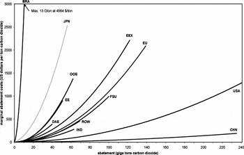
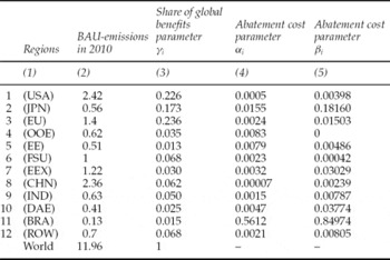
with parameters as listed in the table in the appendix and where abatement qi is the total abatement over 100 years from business-as-usual emissions (BAU emissions). The global benefit parameter b can be interpreted as the discounted global marginal benefit from full cooperation. The value of this parameter was in the original calculations in STACO 37.4 US$ per ton of carbon, in line with older estimates by Tol (Reference Tol1997), but has been updated to 77 US$, reflecting the newest insights by Tol (Reference Tol2005). The regional benefit parameter is γi, representing the shares of the different world regions in global benefits, where  ; αi and βi are regional abatement cost parameters that take on a non-negative value. The regional parameters reflect the differences of 12 world regions: United States of America (USA), Japan (JPN), European Union (EU), other OECD countries (OOE), Eastern European countries (EE), former Soviet Union (FSU), energy exporting countries (EEX), China (CHN), India (IND), dynamic Asian economies (DAE), Brazil (BRA), and ‘rest of the world’ (ROW).Footnote 4 The implications for the different benefit functions can be directly seen from column 3 in the table in the appendix. The large industrialized regions (EU, USA, and JPN) are the main beneficiaries of global abatement, whereas energy-exporting countries (EEX), dynamic Asian economies (DAE), Brazil (BRA), and Eastern European Countries (EE) receive the smallest shares of global benefits. The implications for the different abatement cost functions are more difficult to read from the table in the appendix and are displayed in figure 1.
Marginal abatement cost functions

It is evident that marginal abatement costs vary widely: China, USA, India, and ROW have the flattest curves, whereas Brazil has the steepest, followed by Japan. On average, regions that have low current BAU emissions are costly abaters since further emission reduction is only possible by employing expensive abatement technology. The opposite holds for regions with high current BAU emission levels (see the table in the appendix).
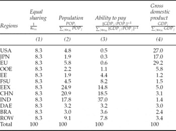
In case of transfers, we consider four different transfer schemes that have played a prominent role in the literature on fair sharing rules in the context of a global climate agreement (Rose et al., Reference Rose1998, Rose and Stevens, Reference Rose and Stevens1998). In our context, these rules relate to the weight λi as explained above. The larger this weight is, the larger is the share that a coalition member receives from the gains of cooperation. The weights implied by the different rules are displayed for the grand coalition in table 2. Therefore, values will be different for other coalitions, though computations are straightforward using the data in table 2.Footnote 5 In the following, we only briefly comment on the four rules and refer the reader to the literature mentioned above for a more comprehensive motivation.
Weights of four transfer schemes*

Notes: *All figures are expressed as a percentage and rounded to the first digit. Base data for computations are taken from Altamirano-Cabrera and Finus (Reference Altamirano-Cabrera and Finus2006). #κm = size of coalition κm, POPi = population in region i, GDPi = gross domestic product in region i.
The transfer scheme ‘equal sharing’ implies in this context that each participant receives the same weight. Given the fact that regions are in many respects very heterogeneous, it is of course debatable whether equal sharing really implies equal and fair treatment.
The transfer scheme ‘population’ acknowledges that all people should benefit equally from cooperation: ‘one man one vote’. Energy exporting countries (EEX), China (CHN), and India (IND) receive high shares since these regions are highly populated. The ‘ability to pay’ rule allocates the gains from cooperation inversely to welfare (measured as GDP) per capita with more or less the same beneficiaries as under the transfer scheme ‘population’.
‘Ability to pay’ links development assistance to environmental policy. Hence, developing countries can make a case that this scheme should be applied as long as welfare is very unevenly distributed, as this is currently the case. Moreover, part of the wealth of industrialized countries has been built on high greenhouse gas emissions in the past, which are responsible for the current stock of carbon. Hence, ecological justice warrants a high share of the global gains from cooperation for developing countries and countries in transition if industrialized countries want these countries joining a climate agreement. This idea is even more powerfully reflected in the scheme ‘population’. From a pure ethical point of view, it appears that this scheme is the most convincing one in favor of developing countries, as it does not have to resort to the argument of development assistance. Moreover, it seems very difficult to argue against the concept of ‘one man one vote’.
The last transfer scheme that we consider is ‘gross domestic product’, which is based on the relative share per region in global GDP. It belongs to the so-called sovereignty rules, because it more or less preserves the current status quo of wealth. Hence, USA, Japan (JPN), and the European Union (EU) receive high shares. The motivation of this transfer scheme is difficult to swallow for developing countries and runs against the idea of linking climate policy to development assistance, as this has been stated by the Framework Convention on Climate Change signed in Rio de Janeiro in 1992. Nevertheless, as we will see, under this scheme transfers (though moderate) flow from industrialized to developing countries and countries in transition.
2.3 Features of the model
In this section, we briefly discuss some features of our model related to payoff function (6) of which the proofs are provided in our working paper (Finus et al., Reference Finus, Sáiz and Hendrix2004).
1. Payoff function (6) implies superadditivity and positive externalities. Superadditivity means that whenever coalitions, say, κℓ and κm merge, so that the coalition structure changes from p to
 , the aggregate payoff to regions in κℓ ∪ κm increases, . Since transfers balance, this is also true for any transfer scheme that we consider in this paper. Positive externalities means that a merger of coalition κℓ and κm raises valuations of outsiders k ∉ {κℓ ∪ κm}, , which also holds in the case of transfers.
2. Superadditivity together with positive externalities implies that global welfare is raised through the merger of coalitions which may be interpreted as increasing the ‘degree of cooperation’. Thus, cooperation raises global welfare and every participant can be better off by using an appropriate transfer scheme.
3. Generally, the advantage of participating in a coalition is that it increases global abatement. This in turn increases benefits from abatement but also increases abatement costs. The relative size of both effects determines whether it pays to join a coalition or to free-ride. Generally, the higher the degree of cooperation, the more attractive it becomes to free-ride due to positive externalities. Therefore, full cooperation and even substantial partial cooperation may be difficult to achieve. This is illustrated in section 3.
 , the aggregate payoff to regions in κℓ ∪ κm increases,
 . Since transfers balance, this is also true for any transfer scheme that we consider in this paper. Positive externalities means that a merger of coalition κℓ and κm raises valuations of outsiders k ∉ {κℓ ∪ κm},
 , which also holds in the case of transfers.
3. Results
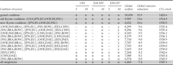
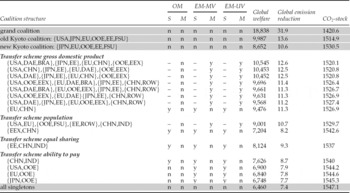
The computations described in section 2 lead to the results shown in table 3 in the case of no transfers and in table 4 for the four different transfer schemes.Footnote 6 Only those coalition structures that are stable are listed, except for the grey rows, which represent important benchmarks. Coalition structures are displayed in a reduced form where only regions that are members of a non-trivial coalition are listed; singleton regions have been omitted. For the no transfer scenario, coalition structures are listed in descending order of global welfare. This also applies to the transfer scenario where structures are listed for each transfer scheme. From the tables the following conclusions can be drawn.
Stable coalition structures in the case of no transfers*

Notes: *Abbreviations of regions as described in subsection 2.2. OM=open membership, EM-MV=exclusive membership majority voting, EM-UV=exclusive membership unanimity voting, S=single coalition game and M=multiple. Global welfare expressed in billion US dollar over 100 years, global emission reduction expressed in percentage from BAU-emissions, assuming BAU-emissions as listed in column 2 in the table in the appendix over 100 years; CO2-stock in giga tons carbon in 2110; y = stable, n = not stable, – = not defined.
Stable coalition structures in the case of transfers*

Note: *Transfer rules as described in section 2.2. For notation, see table 3.
3.1 Gains from cooperation
The possible global gains from cooperation are large in absolute but also in relative terms. Global welfare (defined as the net benefits of climate policies) in the coalition structure ‘grand coalition’ (full cooperation) is three times larger than in the coalition structure ‘all singletons’ (no cooperation). The ‘old Kyoto’ coalition, which comprises all Annex-B regions before the USA withdrew from the Protocol, could close the gap between full and no cooperation by a substantial amount, but is far from being globally optimal. A similar conclusion can be drawn for the ‘new Kyoto’ coalition that misses the USA and therefore yields a lower global welfare than the old Kyoto coalition. However, the old and new Kyoto coalition as well as the grand coalition are not stable, regardless of the treaty design that we consider in this paper. The most successful coalition structure is the first listed in table 4 under the transfer scheme ‘gross domestic product’. This coalition structure emerges if regions can form multiple coalitions and if membership is exclusive. The reason why this institutional setting is conducive to successful cooperation will be taken up below under the heading of ‘transfers’, ‘membership rule’, and ‘multiple coalition structures’.
It is interesting to note that in our model the CO2-stock in the global optimum (1475.1) in 2110, measured in giga tons carbon, translates into a CO2-concentration of 669 ppmv (parts per million volumn). This is in line with for instance Eyckmans and Tulkens (Reference Eyckmans and Tulkens2003), who compute with their CGE-model 644 ppmv in 2100. Our numbers are also in line with the policy scenarios considered in the fourth IPCC report (IPCC, Reference Metz2007) in which targets for climate stabilization range from 350 ppmv to 790 ppmv, translating into an increase of global mean temperature between 2 and 6 degrees celsius.
3.2 Participation
From the number of participants, success of cooperation cannot be inferred. For instance, the coalition structure that comprises only one coalition including the European Union (EU) and China (CHN) (see table 4, last coalition structure listed under the transfer scheme ‘gross domestic product’) implies a larger global welfare than that obtained under many other coalition structures with more coalitions and a higher number of participants as listed under the transfer scheme ‘population’ in table 4, and under no transfers in table 3.
Tables 3 and 4 stress the key role of CHN and USA, as well as India (IND) and ROW for successful cooperation because of their relatively flat marginal abatement cost curve compared to other regions. For instance, in table 3, there are eight multiple coalition structures (displayed in descending order of global welfare) of which the first four include CHN as a coalition member. Also in table 4 under the transfer scheme ‘ability to pay’, three coalitions that do not include CHN as a member yield a lower global welfare than the first listed coalition between CHN and IND. In table 4, all multiple coalition structures under the transfer scheme ‘gross domestic product’, which include the USA, yield a higher global welfare than those listed under no transfers without the USA. However, regions like the EU and JPN are also important as they receive high marginal benefits from cooperation. This calls for high abatement targets (given the assumption of joint welfare maximization; see equation (2)) which is beneficial to all due to positive externalities.
3.3 Transfers
Transfers do make a difference. Many stable coalition structures listed in table 4 generate a higher global welfare, which is particularly true for the transfer scheme ‘gross domestic product’, than those in table 3. The intuition is as follows.
Firstly, the very different structure of both costs and benefits for the regions implies for most coalition structures also a very asymmetric distribution of the gains from cooperation if no transfers are applied. This implies that for some members cooperation would not be profitable (measured against the benchmark no cooperation).Footnote 7 In contrast, all transfer schemes ensure at least profitability.
Secondly, heterogeneity may also cause internal stability to be violated for coalitions with ‘mixed membership’, i.e. coalitions between industrialized and developing countries or countries in transition. On the one hand, it is not attractive for a region with a relatively flat marginal abatement cost curve and low marginal benefits (type 1 regions) to cooperate with other regions because it contributes much to cooperation but benefits only little. Examples include CHN, IND, and ROW. On the other hand, it is not attractive for a region to cooperate with a region that has high marginal benefits and a steep marginal abatement cost curve (type 2 regions) because this implies a high abatement target for the coalition to which type 2 regions contribute only little. Examples include EU and JPN.
Hence, if there are no transfers, coalitions do not comprise of mixed membership (see table 3). Moreover, no stable coalition includes USA. In contrast, if there are transfers, USA is a frequent partner in stable coalitions (see table 4). Moreover, mixed membership is possible, depending on the transfer scheme, including the key players USA, CHN, ROW, EU, and JPN. The scheme ‘gross domestic product’ is clearly superior compared to the other three transfer schemes because it ensures mixed membership. It implies modest transfers from industrialized to other countries. In contrast, the three other transfer schemes imply large transfers. This de facto replaces the asymmetry without transfers with another asymmetry which is more or less reversed, but also not helpful for successful coalition formation.
3.4 Membership rule
The membership rule has a crucial impact on stability and success of cooperation. This is particularly pronounced in the case of no transfers where stable coalition structures only emerge under exclusive membership with unanimity voting (table 3). In the case of transfers, this difference is less pronounced (table 4). Nevertheless, many of the coalition structures with high global welfare are only stable under exclusive membership, though majority voting is sufficient to stabilize these coalition structures.
3.5 Multiple coalition structures
Provided coalition formation is not restricted to a single coalition, coalition structures with multiple coalitions frequently emerge in equilibrium. Multiple coalitions are superior to single coalitions in terms of global welfare. The advantage of multiple coalitions is particularly pronounced in the case of no transfer (table 3) and under the transfer scheme ‘gross domestic product’ (table 4). Only in the case of the transfer schemes ‘equal sharing’ and ‘ability to pay’ (table 4) is there no coalition structure stable when multiple coalitions can be formed. However, some coalition structures are stable if coalition formation is restricted to a single coalition.
4. Summary, conclusions, and extensions
We analyzed coalition formation in the context of global warming. The analysis was based on the stability of coalitions model, STACO, that provides benefit and cost estimates of 12 world regions. We considered several agreement designs: single versus multiple coalitions, open versus exclusive membership with either majority or unanimity voting, and no transfers versus transfers with four different transfer schemes. A wider interpretation of our results allows for the following conclusions.
1. The gains from cooperation as computed by our model are large in absolute and relative terms, which suggests that the lack of cooperation is a serious problem in the context of climate change. The conjecture that a high participation means success is misleading. More important is the inclusion of key players, which in our model are China, USA, India, and ROW due to their flat marginal abatement cost curves, as well as EU and Japan due their high marginal benefits.
2. The effort to get as many countries as possible into one ‘climate boat’ may not be the best strategy in the presence of free-rider incentives. Allowing for separate agreements among regions that have similar interests may foster the success of international agreements. In this light, the position of the USA only to ratify the Kyoto Protocol if developing countries will also join the protocol and take on climate responsibility is open to criticism.Footnote 8 However, their announcement in the aftermaths of their withdrawal that they would pursue their own climate policy cooperating with countries of similar interests may be evaluated positively. At least as an intermediate step, multiple agreements may be useful on the way to a global treaty, as this is often the case with regional trade agreements that lead to more comprehensive agreements at later stages. For the design of post-Kyoto agreements, one possibility would be that developing countries and countries in transition form their own treaty as long as industrialized countries are not prepared to provide enough compensation for these countries to join a single treaty.
3. Certainly, club good agreements (e.g. NATO, European Union, and WTO) may enjoy a higher stability and success than public good agreements, like international environmental agreements, because the benefits from contributions are exclusive to members. However, another reason may be that accession is limited through majority or unanimity voting. Hence, the open membership rule as applied in almost every international environmental treaty should not be taken for granted.
4. Transfers can foster the success of cooperation if actors have asymmetric benefit–cost structures. They can be used to induce participation of regions with cheap abatement options that perceive the benefits from climate policy to be rather low, which is typical for developing countries and countries in transition, together with industrialized countries, which push for high ambitious abatement targets. However, balancing interests between heterogeneous regions is not an easy task. In our setting, it turned out that transfer schemes motivated by some notion of equity are not the most effective for climate policy (measured by the global welfare gain from cooperation). This suggests the importance of also including the stability dimension in the literature on fair sharing, which so far only considered distributional issues.
For future research, we think that three issues (which are underlined in table 1) may be particularly fruitful.
1. Our approach assumed a simultaneous coalition formation process, though in reality signature and ratification of IEAs usually take place sequentially. The sequential move unanimity game of Bloch (Reference Bloch1996) could certainly be a starting point for such an alternative approach, though it seems that conceptual modifications are needed in order to capture what is really going on in negotiations leading to an IEA. Preliminary results from a stylized model with symmetric players in Finus and Rundshagen (Reference Finus and Rundshagen2006) suggest that a sequential process adds another strategic dimension, making successful coalition formation even more difficult due to free-riding.
2. Though the assumption of joint welfare maximization of coalitions (which may be interpreted as a first-best design) is frequently made in the literature, casual empirical evidence suggests that governments do not follow this rule when negotiating abatement targets. Abatement allocation is often not cost-effective and the aggregate level is not optimal from a global point of view (i.e. second-best designs). An alternative approach could model negotiations as a non-cooperative bargaining game over emission reductions, capturing also the political decision process within countries.
Preliminary results that consider a departure from cost-effectiveness and lower coalitional abatement targets in a simple bargaining model suggest that this may well pay from a global point of view (Altamirano-Cabrera et al., Reference Altamirano-Cabrera, Finus and Dellink2008). Second-best designs lead to large stable coalitions that are more successful than small stable coalitions with first-best design. Whether this applies to coalition structures with multiple coalitions remains to be investigated.
3. In line with the literature, we considered several transfer schemes that are related to sharing rules of cooperative game theory. Also in line with the literature, we found that the success depends on the sharing schemes. However, no information is available on other transfer schemes that could yield even more successful stable coalition structures, let alone which transfer scheme would be optimal. By optimal we mean a transfer scheme that stabilizes the coalition structure that generates the largest global welfare among those coalition structures that can be potentially stabilized. For coalition structures with a single coalition, Eyckmans and Finus (Reference Eyckmans and Finus2004) and Weikard (Reference Weikard2005) have independently shown that such a transfer scheme can be constructed, which is illustrated in Carraro et al. (Reference Carraro, Eyckmans and Finus2006). The main problem is to extend this concept to the context of coalition structures with multiple coalitions, which, as we have seen, are often more successful than single coalitions. The main problem is that for multiple coalitions not only internal and external but also intercoalitional stability must be considered where there may be a trade-off between these three dimensions of stability.
Finally, we would like to mention two limitations of our model, which may be taken up in future research.
1. In our model, the incentives for coalition formation are exclusively restricted to costs and benefits from greenhouse gas reduction. On the one hand, this means that equity can only work through the channel of the redistribution of the gains from cooperation via transfers. However, apart from this ‘material payoff’, equity per se may be part of the utility function of agents in the form of ‘non-material’ payoffs. Results from stylized models with symmetric players and a single coalition in Lange and Vogt (Reference Lange and Vogt2003), and Peters and Schuler (Reference Peters and Schuler2006), suggest that equity can be conducive to the success of coalition formation. On the other hand, the literature on issue linkage – initiated by Folmer et al. (Reference Folmer, Mouche and Ragland1993) – suggests that not only monetary transfers but also concessions in other policy issues (e.g. trade, research, and development) can help to balance interests between heterogeneous regions.
It appears that both extensions could do more justice to the role of developing countries and countries in transition for climate change than our analysis. In particular, the discussion of fairness and the link between climate change and development assistance in the form of technology transfers could be analyzed more appropriately.
2. Results of empirical models always depend on the assumption of parameter values. Of course, changes in assumptions will affect quantitative results. However, more important is the question whether they will also affect our qualitative conclusions. In our model, it turns out that qualitative results will not be affected by a change of the global benefit parameter b in the payoff function (6). As mentioned in subsection 2.2, the value in the original calculations in STACO was assumed to be 37.4 US$ per ton carbon, which we updated to 77 US$.Footnote 9 With qualitative conclusions we mean all our results in section 3 and the interpretations derived in section 4 concerning ‘gains from cooperation’, ‘participation’, ‘transfers’, ‘membership rule’, and ‘multiple coalition structures’. Even the composition of stable coalition structures hardly changes. Quantitative results change insofar as equilibrium abatement levels as well global welfare in a given coalition structure are now higher. For instance in the grand coalition, discounted global welfare is 18,838 billion US$ and global emission reduction is 31.9 per cent for b=77 US$ (see tables 3 and 4), whereas for b=37.4 US$ this is 6,031 billion US$ and 21.4 per cent, respectively. However, the relative gains from cooperation measured against the benchmark of no cooperation remain almost the same.
Due to the simple structure of STACO, a similar effect (i.e. an increase of the benefit parameter b) could be observed by lowering the discount rate or lowering abatement costs uniformly as explained in Weikard et al. (Reference Weikard, Finus and Altamirano-Cabrera2006). The former effect could be due to a change of the time preference rate, the latter effect could be due to technological innovation.
There is also some indication that the main qualitative results are unaffected if regional parameters are changed, though membership in coalitions will certainly change (e.g. Finus et al., Reference Finus, Altamirano-Cabrera and Ierland2005). In STACO this concerns the regional benefit parameter γi and the regional cost parameter αi and βi. As the analysis of stable coalition structures depends, even in our simple model, on so many different forces, predictions are difficult. However, we may expect that if the regional benefit parameter γi of say China increased due to more environmental pressure, this would increase the incentive of this country to participate in a climate treaty with industrialized countries. That is, in future China's incentive structure may resemble more that of industrialized countries. This effect may be reinforced if we assume that – despite technological innovations – her abatement cost increases as BAU-emissions increase dramatically due to fast economic development.
In order to treat these uncertain changes systematically over time, two major changes of our model would be required. Firstly, we would need a truly dynamic model of the CGE type, which also includes endogenous growth of emissions and technological innovation. Moreover, stability would have to be tested at each point in time along the entire time path. Secondly, since all changes are uncertain by their very nature, a systematic analysis of uncertainty would be necessary. However, this is beyond the scope of the present paper – considering that currently only few CGE-models with endogenous technological change are around (e.g. Buonanno et al., Reference Buonanno, Carraro and Galeotti2003), so far dynamic stability of coalitions has only been treated in very simple stylized models (e.g. Rubio and Ulph, Reference Rubio and Ulph2007) and a systematic analysis of uncertainty has only been developed for single coalitions (e.g. Dellink et al., Reference Dellink, Finus and Olieman2008).
Emissions, benefit and abatement cost parameters*

Notes: *Input data in STACO-model as described in Finus et al. (Reference Finus, Altamirano-Cabrera and Ierland2005). BAU-Emissions are emissions in the business-as-usual scenario measured in giga tons carbon.
 , then for any coalition κ weights λi are given by
 .