2 Experimental details and phase-averaging technique

2.1 Experimental details

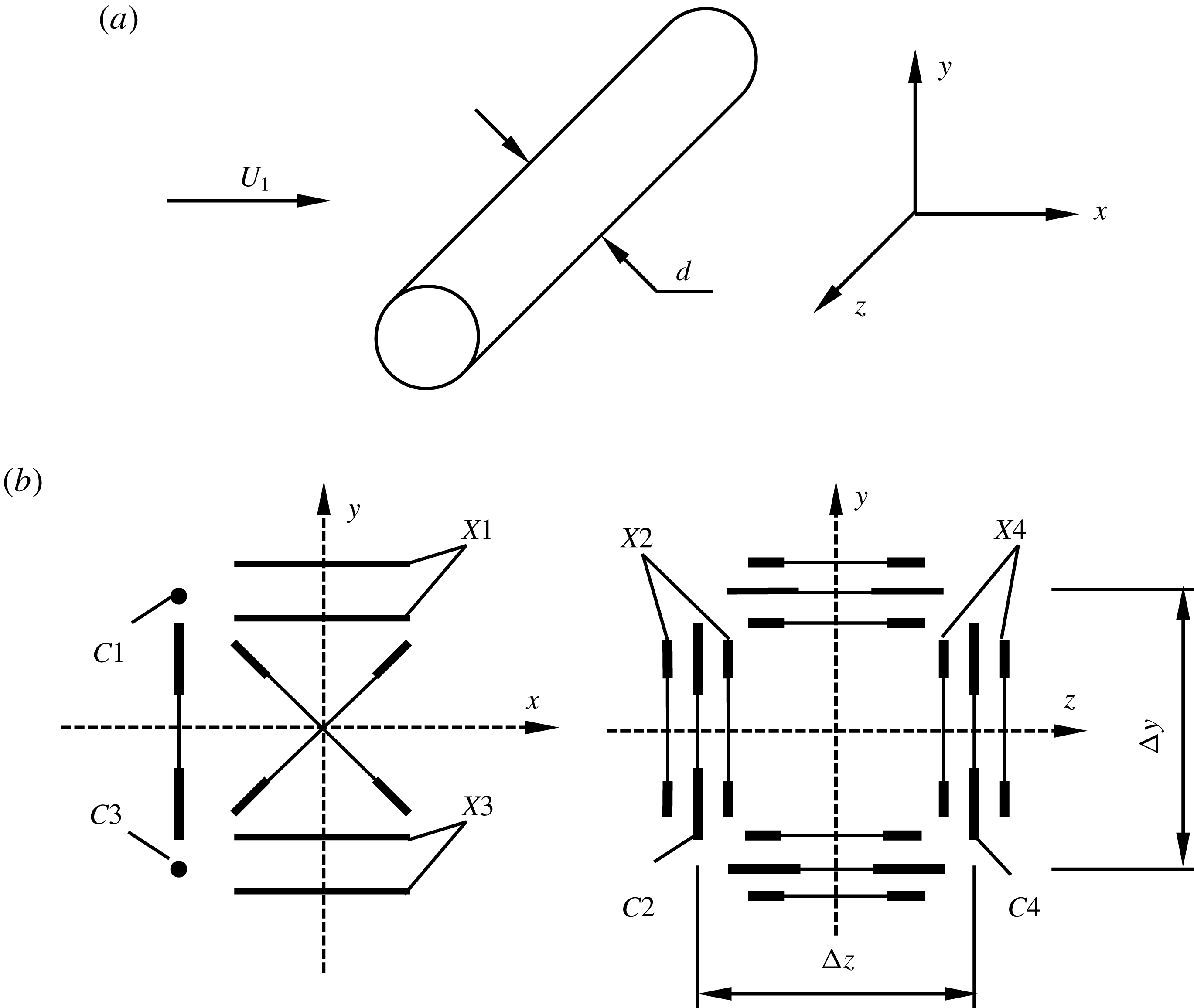
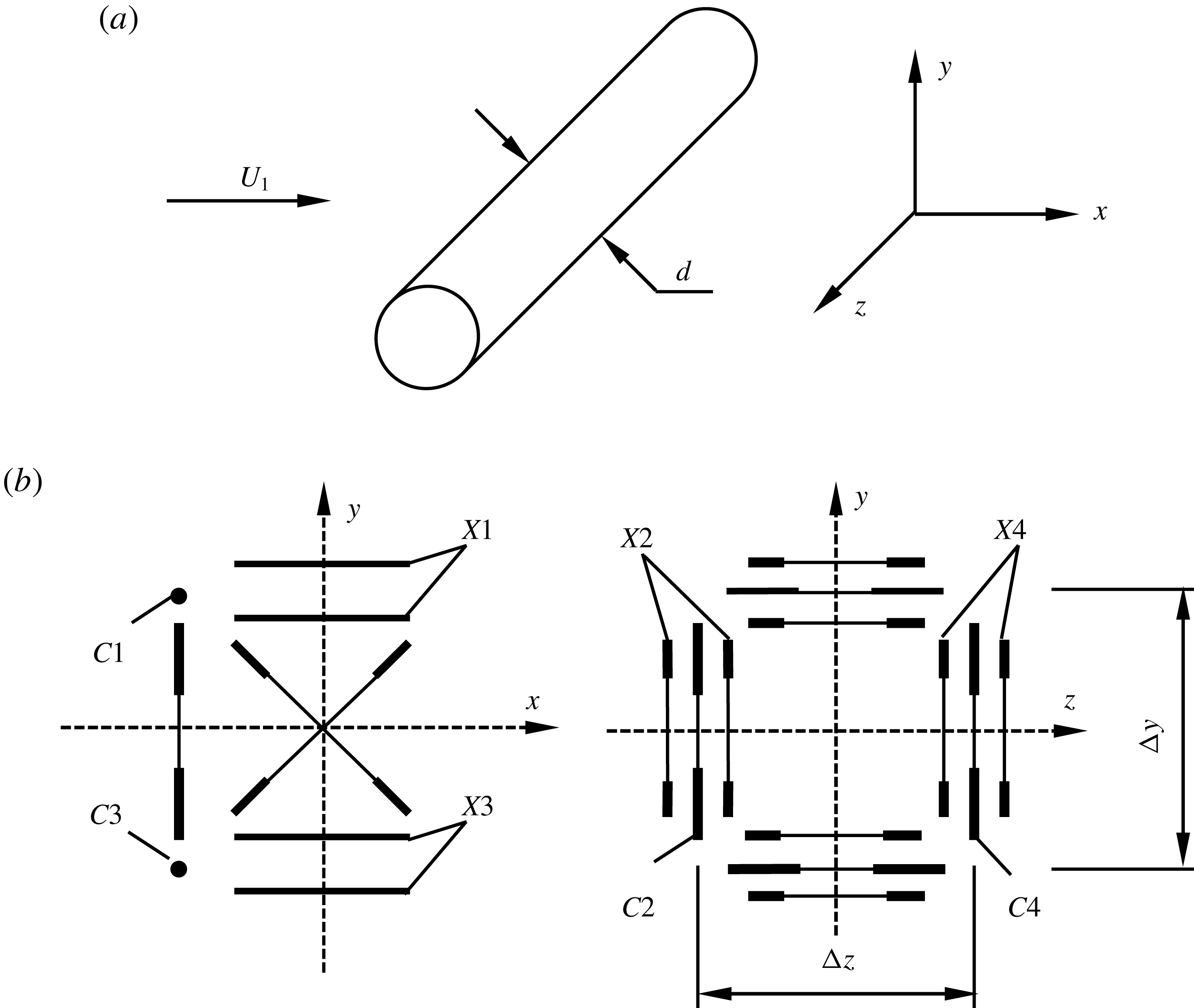
A detailed description of the experimental configuration was given in Chen et al. (Reference Chen, Zhou, Zhou and Antonia2016) and here we briefly recall some important features of the experimental details. Experiments were conducted in an open-loop wind tunnel with a 2.0 m long working section of 1.2 (width) $\times$ 0.8 m (height). A circular cylinder was used to generate the wake. The cylinder is aligned horizontally at the centre of the test section and supported rigidly by two aluminium sharp-edged end plates. The cylinder is made of a 110 cm long smooth brass tube with an outer diameter of 12.7 mm, i.e. with an aspect ratio of approximately 87 and a blockage ratio of 1.6 %. A coiled heating wire with a diameter of approximately 0.5 mm was inserted into a ceramic tube, which was put inside the cylinder as a heating element. The free-stream velocity $U_{1}$ was $3.0~\text{m}~\text{s}^{-1}$ , corresponding to a Reynolds number $Re$ ( $\equiv U_{1}d/\unicode[STIX]{x1D708}$ ) of $2.5\times 10^{3}$ , where $\unicode[STIX]{x1D708}$ is the kinematic viscosity. Measurements were conducted within the cylinder mid-span plane at $x/d=10$ , 20 and 40, where $x$ is the streamwise distance from the cylinder axis (figure 1 a). This study focuses on the flow field at $x/d=10$ where the Kármán vortex is more organized than at the two downstream positions.

Figure 1.

(a) Experimental arrangement and the coordinate system; (b) side (left) and front (right) view of the probe.

The unheated cylinder wake has been shown to be statistically symmetrical about the centreline, e.g. by Zhou et al. (Reference Zhou, Razali, Zhou, Chua and Cheng2009). As a result, the present measurements were made only on one side of the centreline, i.e. $y/d=-0.2{-}2.8$ , with a transverse measurement increment of approximately $0.2d$ . The coordinate system and some symbols are defined in figure 1(a). The maximum mean temperature excess $\unicode[STIX]{x1D6E9}_{0}$ , relative to the ambient fluid, is approximately $1.6\,^{\circ }\text{C}$ on the wake centreline ( $y/d=0$ ). This excess is small enough to avoid any buoyancy effects, and hence allows the temperature to be treated as a passive scalar.

A probe consisting of four X-wires (X1–X4 in figure 1 b) and four cold wires (C1–C4 in figure 1 b) was used to measure simultaneously the fluctuating velocity $u_{i}$ , vorticity $\unicode[STIX]{x1D714}_{i}$ , temperature $\unicode[STIX]{x1D703}$ and temperature gradient $\unicode[STIX]{x1D703}_{,i}$ at nominally the same spatial point, where $i$ ( $=1$ , 2 and 3) represents the $x$ , $y$ and $z$ directions, respectively. Please refer to Chen et al. (Reference Chen, Zhou, Zhou and Antonia2016) for more details about the probe and its performance in measuring $u_{i}$ , $\unicode[STIX]{x1D714}_{i}$ and $\unicode[STIX]{x1D703}$ .

2.2 Phase-averaging technique

A phase-averaging technique is used to calculate the statistics of the examined quantity at a specified phase. The technique is the same as that used in Chen et al. (Reference Chen, Zhou, Zhou and Antonia2016) and will not be repeated here. Briefly, the instantaneous quantity $\unicode[STIX]{x1D6E4}$ may be viewed as the sum of the time-averaged component $\overline{\unicode[STIX]{x1D6E4}}$ and the fluctuating component $\unicode[STIX]{x1D6FD}$ , which can be further decomposed into a coherent fluctuation $\widetilde{\unicode[STIX]{x1D6FD}}$ and a remainder $\unicode[STIX]{x1D6FD}_{r}$ , namely

(2.1) $$\begin{eqnarray}\unicode[STIX]{x1D6FD}=\widetilde{\unicode[STIX]{x1D6FD}}+\unicode[STIX]{x1D6FD}_{r}.\end{eqnarray}$$

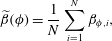
The coherent part $\widetilde{\unicode[STIX]{x1D6FD}}$ reflects the effect from the large-scale coherent structures, while the remainder $\unicode[STIX]{x1D6FD}_{r}$ reflects largely the random incoherent motions in the flow. The phase average of the fluctuating quantity $\unicode[STIX]{x1D6FD}$ is given by

(2.2) $$\begin{eqnarray}\widetilde{\unicode[STIX]{x1D6FD}}(\unicode[STIX]{x1D719})=\frac{1}{N}\mathop{\sum }_{i=1}^{N}\unicode[STIX]{x1D6FD}_{\unicode[STIX]{x1D719},i},\end{eqnarray}$$

where $\unicode[STIX]{x1D719}$ represents the phase, and $N$ is the number of detected vortex shedding periods, which is presently approximately 1980. When the cylindrical coordinate is used, with the vortex centre at $r=0$ , the value of $\widetilde{\unicode[STIX]{x1D6FD}}(r)$ is given by

(2.3) $$\begin{eqnarray}\widetilde{\unicode[STIX]{x1D6FD}}(r)=\frac{1}{N}\mathop{\sum }_{i=1}^{N}\unicode[STIX]{x1D6FD}_{r,i}.\end{eqnarray}$$

3 Temperature and velocity fluctuations within the Kármán vortex

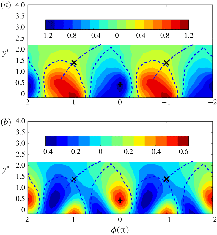
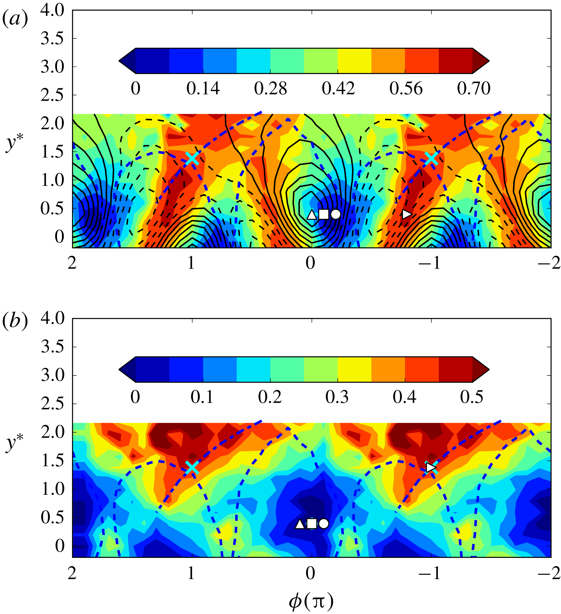
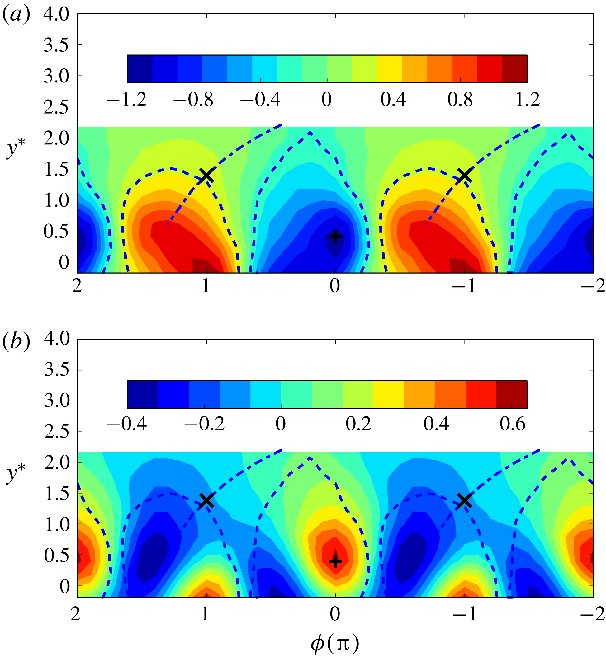
In order to have a visual perspective of the Kármán vortex and the associated temperature field, we start by plotting (figure 2) the colour-filled iso-contours of $\widetilde{\unicode[STIX]{x1D714}}_{3}^{\ast }$ and $\widetilde{\unicode[STIX]{x1D703}^{\ast }}$ . Hereafter, an asterisk denotes normalization by $d$ , $U_{1}$ and/or $\unicode[STIX]{x1D6E9}_{0}$ . This information was first obtained by Chen et al. (Reference Chen, Zhou, Zhou and Antonia2016) and is simply re-presented here as a reference. The phase $\unicode[STIX]{x1D719}$ can be interpreted in terms of a longitudinal distance based on Taylor’s hypothesis; the range $\unicode[STIX]{x1D719}=0{-}2\unicode[STIX]{x03C0}$ corresponds to the average vortex wavelength. The Kármán vortex centre and saddle points, identified from the phase-averaged sectional streamlines (not shown), are marked by ‘ $+$ ’ and ‘ $\times$ ’ respectively. The vortex boundary which has been arbitrarily assumed to correspond to approximately 25 % of the maximum concentration of $\widetilde{\unicode[STIX]{x1D714}_{3}}^{\ast }$ in figure 2(a) is represented as a thick dashed line in figure 2(b). The inclined dash-dotted line passing through the saddle point represents the diverging separatrix. Clearly, the opposite-signed Kármán vortices are alternatively arranged along the wake centreline (figure 2 a). The vorticity contours are inclined as a result of the vigorous interaction between neighbouring vortices. The high temperature warm fluid (positive $\widetilde{\unicode[STIX]{x1D703}^{\ast }}$ ) is distributed within the Kármán vortices, while the cool fluid (negative $\widetilde{\unicode[STIX]{x1D703}^{\ast }}$ ) entrained by the vortices from the ambient free stream occupies the alley way between consecutive vortices. Two large-scale warm/cool temperature fronts emerge: one is along the direction of the diverging separatrix, which is similar to Antonia et al.’s (Reference Antonia, Chambers, Britz and Browne1986) observation in a plane jet; another is immediately downstream of the vortex roll. The different effects of these two fronts on the temperature field will be discussed in § 5. Our primary objective here is to focus on the statistics of the temperature and velocity fields within the Kármán vortex and how they differ from the conventional statistics that give equal weighting to flow regions both within and outside the vortex.

Figure 2.

(a) Phase-averaged spanwise vorticity $\widetilde{\unicode[STIX]{x1D714}_{3}}^{\ast }$ and (b) temperature fluctuation $\widetilde{\unicode[STIX]{x1D703}^{\ast }}$ .

Figure 3.

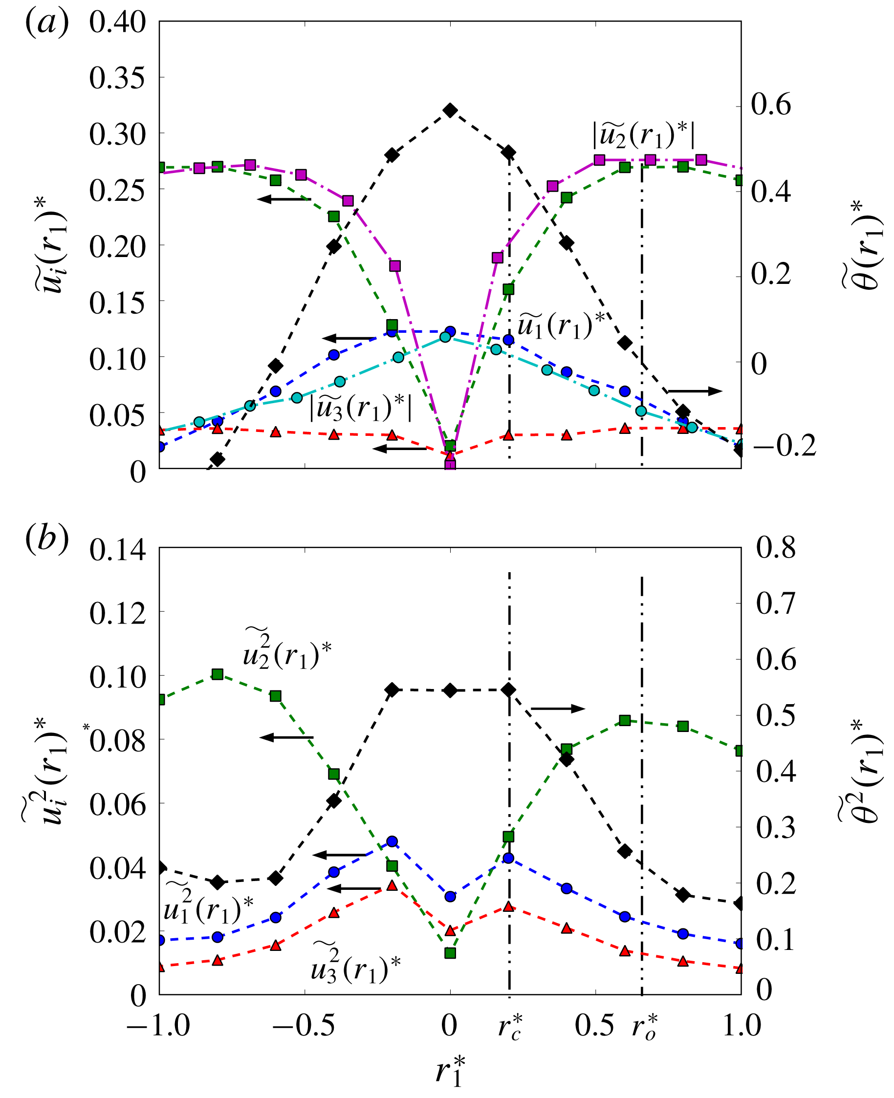
The distributions of the phase-averaged (a) mean and (b) mean-square fluctuating velocities and temperature within the vortex in the $x$ -direction through the vortex centre. The data of $\widetilde{u_{1}}(r_{1})^{\ast }$ and $\widetilde{u_{2}}(r_{1})^{\ast }$ in Zhou & Antonia (Reference Zhou and Antonia1993) (dash-dotted line) are included in (a) for comparison. The vertical lines mark the inner and outer core radii $r_{c}^{\ast }$ and $r_{o}^{\ast }$ , respectively.

Figure 4.

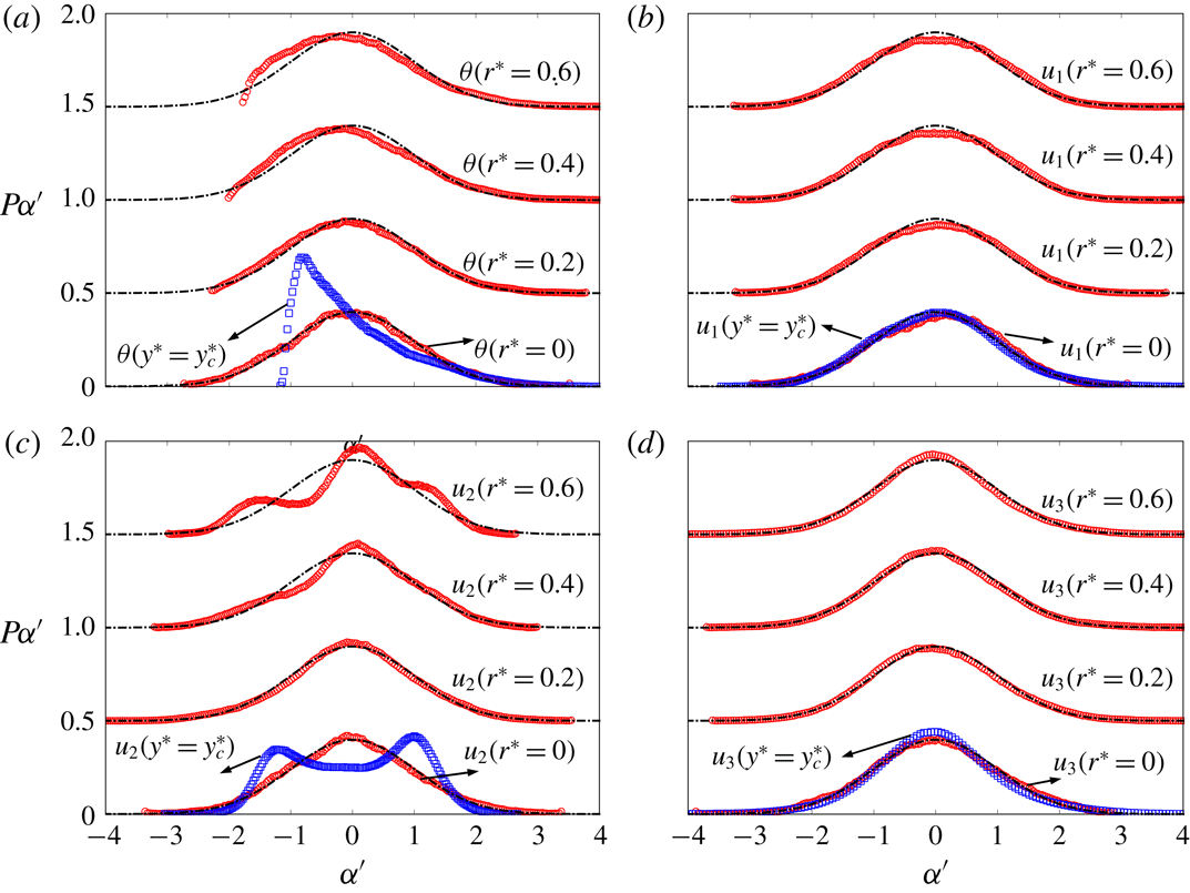
The p.d.f.s (red circles) of (a) fluctuating temperature and (b–d) velocities at different distances ( $r^{\ast }=0{-}0.6$ ) from the Kármán vortex centre ( $\unicode[STIX]{x1D719}=0$ , $y^{\ast }=y_{c}^{\ast }$ ). The conventional p.d.f.s (blue squares) at the lateral position of the vortex centre ( $y^{\ast }=y_{c}^{\ast }$ ) are also included for comparison. The black dash-dotted lines are Gaussian distribution.

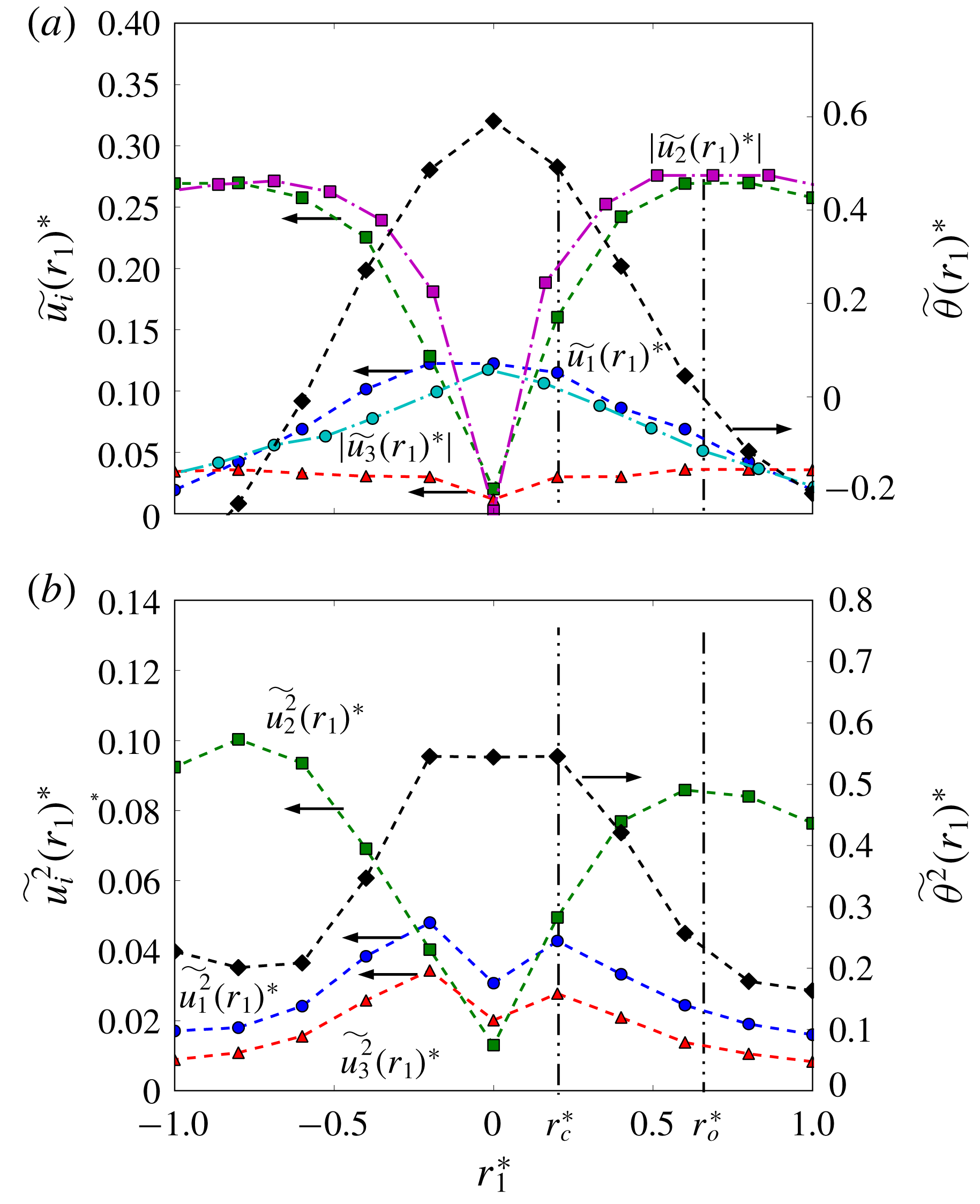
Zhou & Antonia (Reference Zhou and Antonia1993) examined, based on vortex detections, the distribution of the conditionally averaged circumferential velocity, along the streamwise direction through the vortex centre, within the Kármán vortex and found that this velocity follows the Oseen vortex model (e.g. Granger Reference Granger1985, p. 475) reasonably well. Figure 3 presents the distributions of the three phase-averaged components $\widetilde{u_{i}}(r_{1})^{\ast }$ ( $i=1$ , 2 and 3) of the fluctuating velocity vector, along with $\widetilde{\unicode[STIX]{x1D703}}(r_{1})^{\ast }$ , where $r_{1}^{\ast }$ is the streamwise distance from the vortex centre calculated using Taylor’s hypothesis. The distributions of $\widetilde{u_{1}}(r_{1})^{\ast }$ and $\widetilde{u_{2}}(r_{1})^{\ast }$ in Zhou & Antonia (Reference Zhou and Antonia1993) are also included for comparison. The present distributions $\widetilde{u_{1}}(r_{1})^{\ast }$ and $\widetilde{u_{2}}(r_{1})^{\ast }$ agree reasonably well with those obtained by Zhou & Antonia (Reference Zhou and Antonia1993). The value of $\widetilde{u_{2}}(r_{1})^{\ast }$ increases rapidly and almost linearly near the vortex centre and reaches a maximum before decreasing slowly. The slightly more rapid rise in $\widetilde{u_{2}}(r_{1})^{\ast }$ of Zhou & Antonia (Reference Zhou and Antonia1993) near the vortex centre is ascribed to the fact that these authors detected only the rather strong vortices. The region $r^{\ast }\leqslant r_{c}^{\ast }$ ( ${\approx}0.2$ ), where $\widetilde{u_{2}}(r_{1})^{\ast }$ rises rapidly and approximately linearly and the coherent motion behaves like a rigid body, may be referred to as the inner core of the vortex. The region at larger $r^{\ast }$ which is enclosed by the radius $r_{0}^{\ast }\approx 0.65$ , at which $\widetilde{u_{2}}(r_{1})^{\ast }$ reaches the maximum, is identified with the outer core of the vortex. As will be shown later, the inner core region possesses some unique features which are absent in the outer core region. The $\widetilde{u_{1}}(r_{1})^{\ast }$ shows its maximum magnitude at the vortex centre and drops gradually with increasing $r_{1}^{\ast }$ . The occurrence of the maximum $\widetilde{u_{1}}(r_{1})^{\ast }$ at the vortex centre is consistent with Zhou & Antonia’s (Reference Zhou and Antonia1992) finding that the vortex convection velocity at the vortex centre is larger than the local mean velocity. The magnitude of $\widetilde{u_{3}}(r_{1})^{\ast }$ is rather small compared to that of $\widetilde{u_{1}}(r_{1})^{\ast }$ or $\widetilde{u_{2}}(r_{1})^{\ast }$ . This is reasonable. Being mostly induced by the rib structures and the distorted spanwise vortices, $u_{3}$ is statistically randomly orientated; as a result, the positive and negative $u_{3}$ tend to cancel each other. The value of $\widetilde{\unicode[STIX]{x1D703}}(r_{1})^{\ast }$ displays its maximum at the vortex centre and decreases with increasing $r_{1}^{\ast }$ , which agrees internally with the concentric vorticity and temperature iso-contours within the vortex (figure 2 b). It is interesting to note that the radial position of $\widetilde{\unicode[STIX]{x1D703}}(r_{1})^{\ast }\approx 0$ coincides approximately with $r_{0}^{\ast }$ . This observation suggests that the rotational motion or coherence needs to be adequately strong to retain heat or the scalar within the vortex.

The radial distribution of the phase-averaged mean-square values of the fluctuating velocities and temperature are shown in figure 3(b). The distributions of $\widetilde{u_{1}^{2}}(r_{1})^{\ast }$ have a local minimum at the vortex centre. As $r_{1}^{\ast }$ increases, $\widetilde{u_{2}^{2}}(r_{1})^{\ast }$ is similar to $\widetilde{u_{2}}(r_{1})^{\ast }$ with a maximum at approximately $r_{0}^{\ast }$ , while $\widetilde{u_{1}^{2}}(r_{1})^{\ast }$ and $\widetilde{u_{3}^{2}}(r_{1})^{\ast }$ reach their maxima rapidly at $r_{1}^{\ast }=0.2$ , i.e. the edge of the inner core, before decreasing slowly beyond this location. Within the inner core ( $r_{1}^{\ast }\leqslant r_{c}^{\ast }$ ), $\widetilde{\unicode[STIX]{x1D703}^{2}}(r_{1})^{\ast }$ is approximately constant, suggesting that the root-mean-square (r.m.s.) scalar field is more homogeneous within the inner core than the r.m.s. velocity field.

Figure 4 compares the p.d.f.s of $u_{i}$ and $\unicode[STIX]{x1D703}$ at different radial distances ( $r^{\ast }=0$ , 0.2, 0.4, 0.6) from the vortex centre, i.e. $y^{\ast }=y_{c}^{\ast }=0.4$ and $\unicode[STIX]{x1D719}=0$ (figure 2 a). Their conventional p.d.f.s at the same $y^{\ast }$ position as the vortex centre are also shown for comparison. All the data are centred, that is, the mathematical expectation has been subtracted, and then are normalized by the standard deviation, viz. $\unicode[STIX]{x1D6FC}^{\prime }=(\unicode[STIX]{x1D6FC}-E(\unicode[STIX]{x1D6FC}))/\unicode[STIX]{x1D70E}_{\unicode[STIX]{x1D6FC}}$ where $\unicode[STIX]{x1D6FC}$ denotes $u_{i}(r)$ , $\unicode[STIX]{x1D703}(r)$ , $u_{i}$ and $\unicode[STIX]{x1D703}$ at $y^{\ast }=y_{c}^{\ast }$ ; $\unicode[STIX]{x1D70E}_{\unicode[STIX]{x1D6FC}}$ stands for the standard deviation of $\unicode[STIX]{x1D6FC}$ , and $E(\unicode[STIX]{x1D6FC})$ is the mathematical expectation. Note that $E(\unicode[STIX]{x1D6FC})$ is 0 for $u_{i}$ and $\unicode[STIX]{x1D703}$ , and equal to $\widetilde{\unicode[STIX]{x1D6FC}}(r)$ for $u_{i}(r)$ and $\unicode[STIX]{x1D703}(r)$ . After such standardization, all the examined fluctuations $\unicode[STIX]{x1D6FC}^{\prime }$ have a zero mean and a standard deviation of unity so that their p.d.f.s can be compared with a standard Gaussian distribution where the mean and standard deviation are zero and unity, respectively. An impressive result is that all the p.d.f.s of the temperature and velocity fluctuations at the Kármán vortex centre, i.e. $P_{\unicode[STIX]{x1D703}(r^{\ast }=0)}$ and $P_{u_{i}(r^{\ast }=0)}$ , follow the Gaussian distribution closely. In contrast, their conventional counterparts, i.e. $P_{\unicode[STIX]{x1D703}}$ and $P_{u_{i}}$ , exhibit different distributions, especially $P_{u_{2}}$ and $P_{\unicode[STIX]{x1D703}}$ ; $P_{u_{1}(r^{\ast }=0)}$ appears to be slightly more negatively skewed than $P_{u_{1}}$ , which is probably linked to the effect of the streamwise convention velocity of the vortex centre. As commented earlier, the convection velocity at the vortex centre is greater than the local mean velocity. The distributions of $P_{u_{2}}$ and $P_{\unicode[STIX]{x1D703}}$ reflect the effect of the coherent motions in the flow. Specifically, $P_{\unicode[STIX]{x1D703}}$ exhibits a sharp cutoff on its left side due to the presence of the cool fluid (figure 2 b). This is confirmed by the observation that the cutoff temperature (obtained after adding the mean temperature at this $y^{\ast }$ position to $\unicode[STIX]{x1D703}$ ) is very close to the ambient temperature. The twin peaks in $P_{u_{2}}$ , located at approximately the same magnitude of $u_{2}^{\prime }$ , reflect the positive and negative lateral velocities on either side of the Kármán vortex centre. The symmetric $P_{u_{3}}$ with respect to $u_{3}^{\prime }=0$ reflects the spanwise symmetry of the plane wake. The higher value of $P_{u_{3}}$ near 0 than the Gaussian distribution is ascribed to the higher intermittency of $u_{3}$ . This is confirmed by the larger kurtosis of $u_{3}$ relative to the Gaussian value at this $y^{\ast }$ , which will be shown later in this section. This is likely due to the fact that $u_{3}$ is mostly induced by the rib structures and the distorted spanwise vortices in the near wake.

When $r^{\ast }$ reaches 0.2, $P_{\unicode[STIX]{x1D703}(r^{\ast }=0.2)}$ and $P_{ui(r^{\ast }=0.2)}$ are still close to the Gaussian distribution. However, beyond the inner core region, say at $r^{\ast }=0.4$ and 0.6, the p.d.f.s of both velocity and temperature fluctuations depart appreciably from the Gaussian distribution and the departure becomes more pronounced as $r^{\ast }$ increases. This difference between the p.d.f.s at $r^{\ast }=0.2$ and at $r^{\ast }\geqslant 0.4$ is particularly evident for the p.d.f.s of $\unicode[STIX]{x1D703}(r^{\ast })$ (figure 4 a) and $u_{2}(r^{\ast })$ (figure 4 c). The result is fully consistent with what figure 3(b) indicates, that is, the inner core region ( $r_{1}^{\ast }\leqslant r_{c}^{\ast }$ ) of the vortex is markedly different from the outer core.

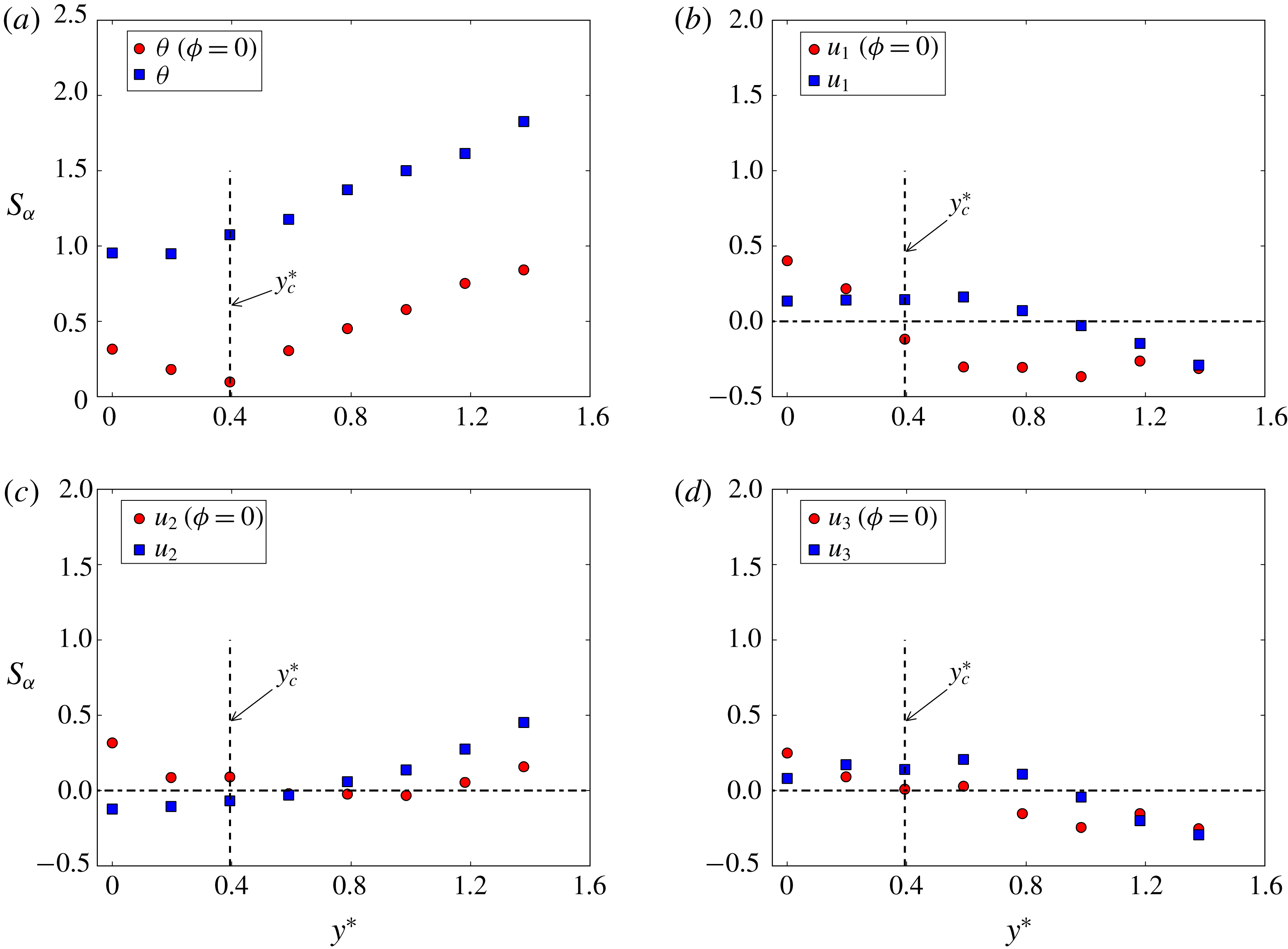
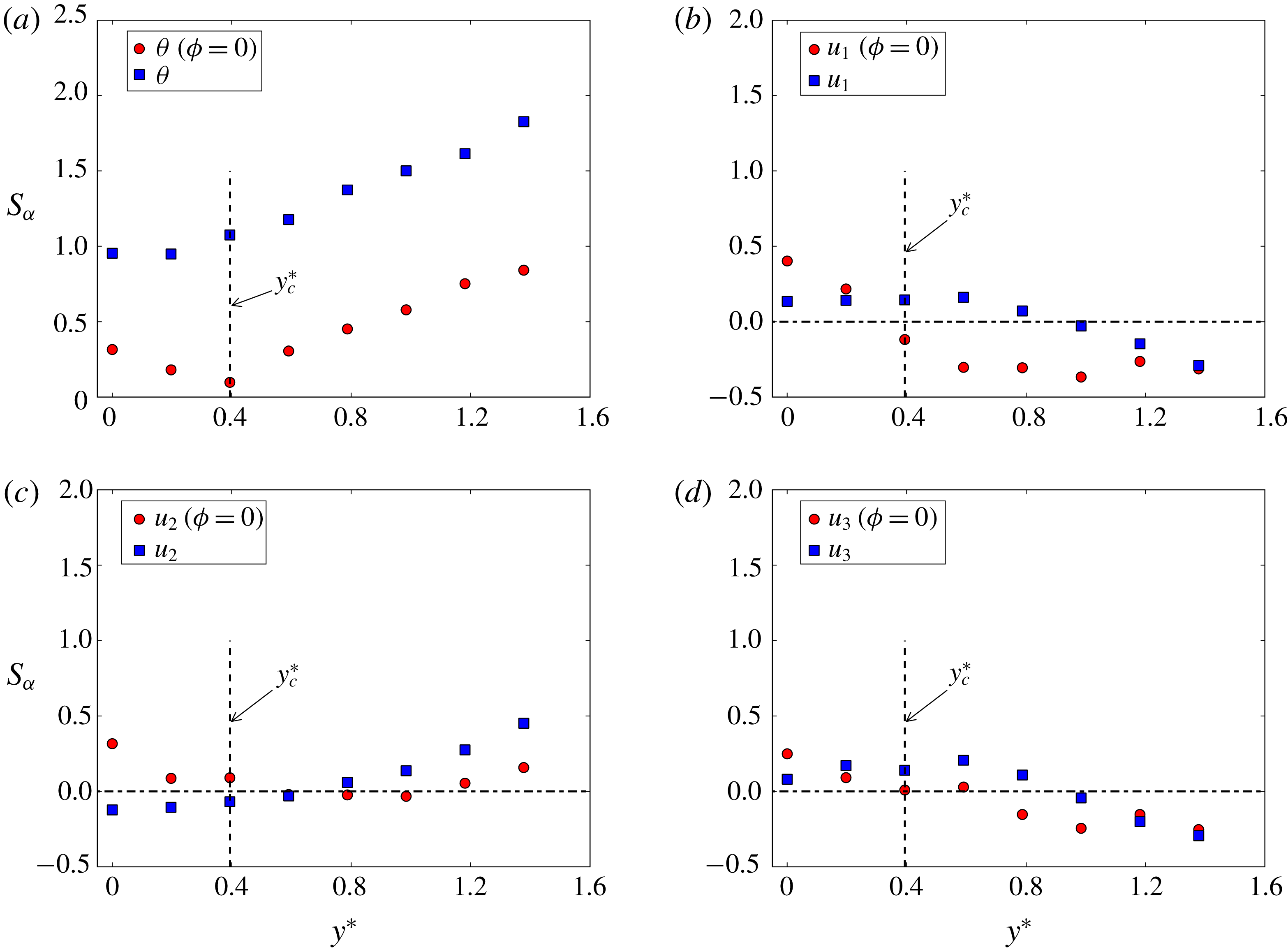
The higher moments such as skewness and kurtosis of $u_{i}$ and $\unicode[STIX]{x1D703}$ may also provide important insight into the physical characteristics of the vortex. Figure 5 shows the lateral distributions of the skewness ( $S$ ) of $\unicode[STIX]{x1D703}(\unicode[STIX]{x1D719}=0)$ and $u_{i}(\unicode[STIX]{x1D719}=\unicode[STIX]{x1D703})$ across the vortex, as well as $\unicode[STIX]{x1D703}$ and $u_{i}$ at the same $y^{\ast }$ . In figure 5(a), the distribution of $S_{\unicode[STIX]{x1D703}(\unicode[STIX]{x1D719}=0)}$ is closer to 0 than $S_{\unicode[STIX]{x1D703}}$ at each $y^{\ast }$ position, particularly at the vortex path ( $y^{\ast }=y_{c}^{\ast }$ ). This observation is consistent with figure 4(a) in which $P_{\unicode[STIX]{x1D703}}$ is apparently more positively skewed; $S_{u_{i}(\unicode[STIX]{x1D719}=0)}$ is close to 0 at $y_{c}^{\ast }$ but gradually departs from 0 as $y^{\ast }$ is away from $y_{c}^{\ast }$ , which conforms to the finding in figure 4(b–d). The $y^{\ast }$ positions corresponding to $S_{u_{i}}\approx 0$ are generally larger than $y_{c}^{\ast }$ , probably due to the effect of the saddle region outside the vortex. Note that the saddle point occurs at $y^{\ast }\approx 1.4$ (figure 2), larger than $y_{c}^{\ast }(=0.4)$ . It is worth noting that the distributions of $S_{u_{1}}$ and $S_{u_{3}}$ are very similar, but distinct from the distribution of $S_{u_{2}}$ . 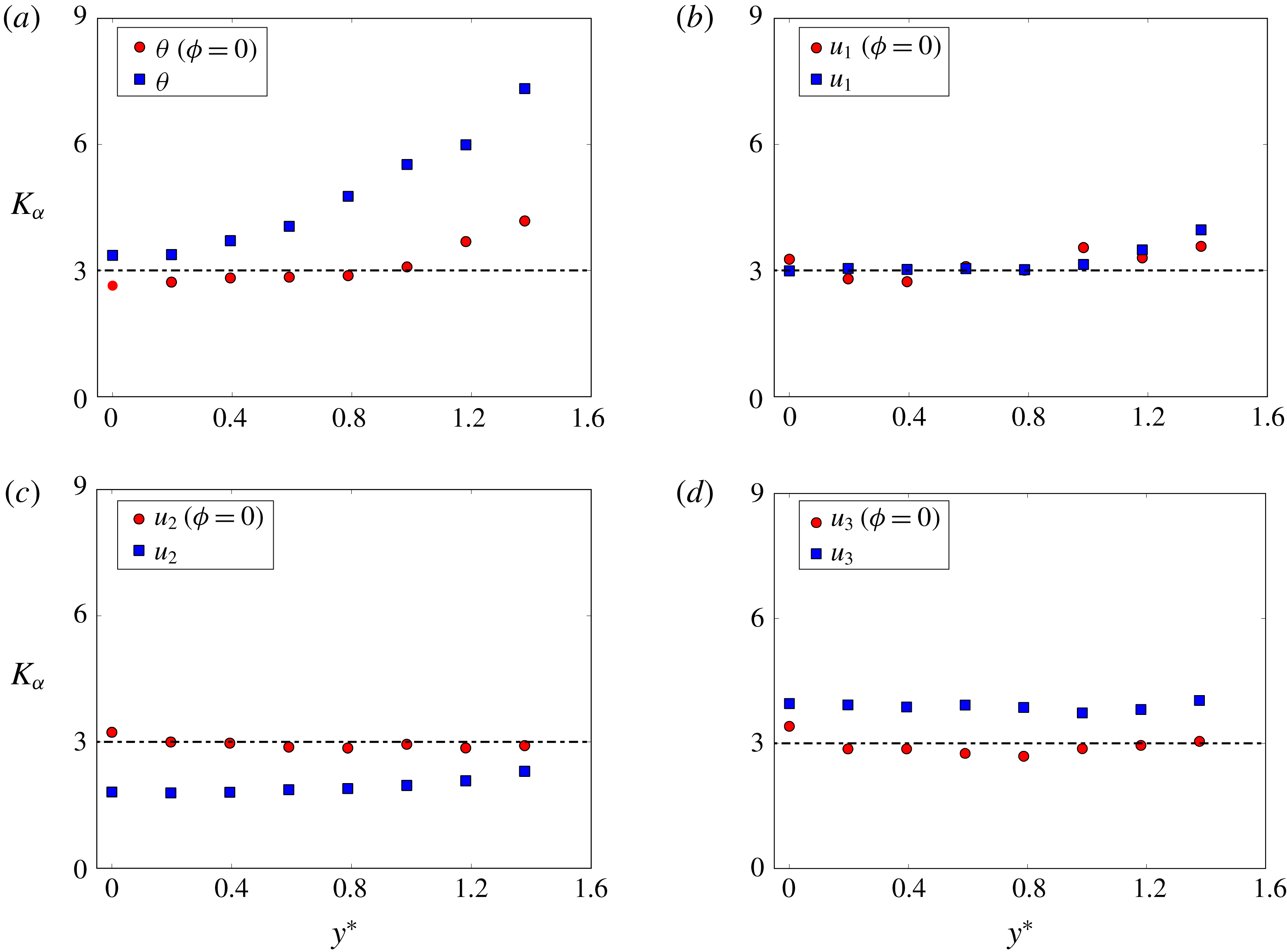This feature is also reflected in the p.d.f.s of $u_{i}$ in figure 4(b–d). The kurtosis ( $K$ ) of $\unicode[STIX]{x1D703}(\unicode[STIX]{x1D719}=0)$ (figure 6 a) is closer to the Gaussian value of 3 than the conventional kurtosis $K_{\unicode[STIX]{x1D703}}$ at all $y^{\ast }$ positions. For the velocity field (figure 6 b–d), $K_{u_{i}}$ deviates from the value of 3, except for $K_{u_{1}}$ , but all the magnitudes of $K_{u_{i}(\unicode[STIX]{x1D719}=0)}$ are reasonably close to 3.

Figure 5.

Distribution of skewness of temperature and velocity fluctuations (red circles) within a Kármán vortex in $y^{\ast }$ direction across the vortex centre ( $\unicode[STIX]{x1D719}=0$ ). The conventional skewness is shown for comparison (blue squares). (a) Temperature fluctuation, (b–d) velocity fluctuations. The vertical dashed line marks the lateral position corresponding to the vortex centre.

Figure 6.

Distribution of kurtosis of temperature and velocities (red circles) within the Kármán vortex in $y^{\ast }$ direction across the vortex centre ( $\unicode[STIX]{x1D719}=0$ ). The conventional kurtosis is shown (blue squares) for comparison. (a) Temperature fluctuation, (b–d) velocity fluctuations. The horizontal dashed line marks the value of 3, the kurtosis of a Gaussian distribution.

Figure 7.

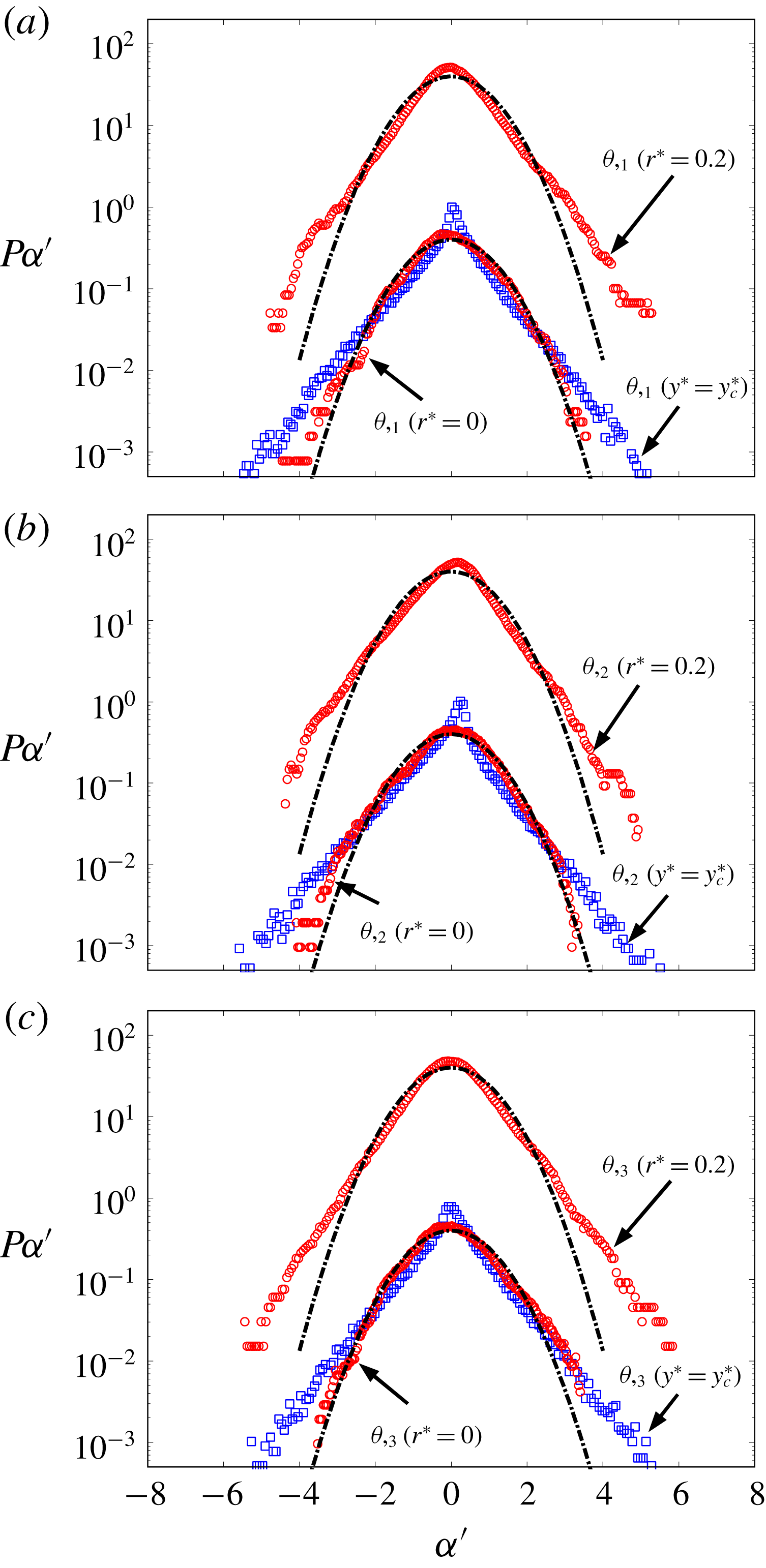
Comparison between the p.d.f.s of the three components of the temperature gradient at different distances ( $r^{\ast }=0$ and 0.2) from the vortex centre and Gaussian distribution. The conventional p.d.f.s at the same lateral position of the vortex centre are also included. The dash-dotted lines are the Gaussian distributions.

In summary, the statistics of the velocity and temperature fields within the Kármán vortex are quite different from the corresponding conventional statistics. The p.d.f.s of the fluctuating temperature and velocity components within the vortex, especially within the inner core region, are characterized approximately by the Gaussian distribution. The physics underpinning this phenomenon is linked to the isolated nature of the random and relatively small-scale turbulence within the Kármán vortex, that is, this turbulence is sheltered from the effect of the coherent structures outside the vortex. This will be discussed in detail in § 5.

4 The p.d.f.s of small-scale temperature gradient and vorticity within the Kármán vortex

The properties of the small scales within the Kármán vortex are examined in this section via the statistics of vorticity and temperature derivatives. Some remarks are due in connection with the spatial resolution of the probe before we proceed with our examination of the small-scale temperature gradient and vorticity inside the vortex. In the study, the streamwise derivatives of the velocity and temperature fluctuations are estimated using Taylor’s hypothesis, i.e. $\unicode[STIX]{x0394}x_{1}\approx -\unicode[STIX]{x0394}tU_{c}$ where $U_{c}=0.87U_{1}$ is the averaged convection velocity of the vortices (Zhou & Antonia Reference Zhou and Antonia1992) and $\unicode[STIX]{x0394}t=1/f_{samp}$ . The use of Taylor’s hypothesis in the present flow has been validated by Mi & Antonia (Reference Mi and Antonia2010) in the near wake of a circular cylinder at a similar Reynolds number. The spatial resolution of measurements in the $x$ , $y$ ,  $z$ directions are estimated to be approximately $5.8\unicode[STIX]{x1D702}$ , $11\unicode[STIX]{x1D702}$ , $15\unicode[STIX]{x1D702}$ , respectively, where $\unicode[STIX]{x1D702}\equiv (\unicode[STIX]{x1D708}^{3}/\bar{\unicode[STIX]{x1D700}})^{1/4}$ is the Kolmogorov length scale on the centreline and $\bar{\unicode[STIX]{x1D700}}$ is approximated by assuming transverse homogeneity in the $y$ – $z$ plane, instead of isotropy. The assumption of homogeneity has been shown (Lefeuvre et al. Reference Lefeuvre, Thiesset, Djenidi and Antonia2014) to provide a better estimation of the mean turbulent energy dissipation rate in the near wake. It has been previously established that the optimum spatial resolution for velocity derivatives is $3{-}5\unicode[STIX]{x1D702}$ (e.g. Shafi & Antonia Reference Shafi and Antonia1997; Zhou, Pearson & Antonia Reference Zhou, Pearson and Antonia2001; Zhou et al. Reference Zhou, Zhou, Yiu and Chua2003); a larger wire separation can cause attenuated velocity derivatives, while a smaller wire separation may overestimate the velocity derivatives because of the electronic noise contamination. The relatively coarse spatial resolution of the probe in the $y$ and $z$ directions may attenuate the high wavenumber range of the power spectrum of the vorticity (e.g. Zhu & Antonia Reference Zhu and Antonia1996). However, it is worth pointing out that the inadequate spatial resolution of the probe is not a problem for the qualitative comparison of the p.d.f.s conducted in this section since both $\unicode[STIX]{x1D703}_{,i}$ and $\unicode[STIX]{x1D703}_{,i}(r^{\ast })$ or $\unicode[STIX]{x1D714}_{i}$ and $\unicode[STIX]{x1D714}_{i}(r^{\ast })$ are attenuated basically at the same level.

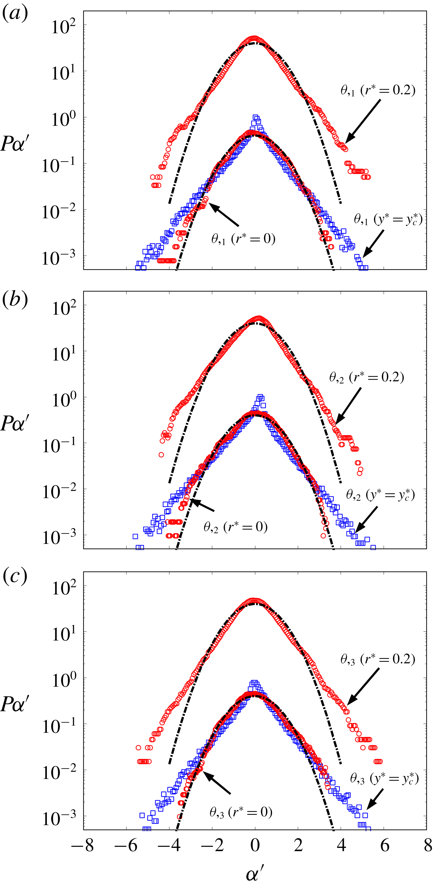
Figure 7 shows the p.d.f.s of the temperature derivatives at the vortex centre and at $r^{\ast }=0.2$ , along with the conventional p.d.f.s at the same $y^{\ast }$ position as the vortex centre. For convenience, we use the notation $\unicode[STIX]{x1D703}_{,i}\equiv \unicode[STIX]{x2202}\unicode[STIX]{x1D703}/\unicode[STIX]{x2202}x_{i}$ ( $i=1$ , 2 and 3). A semilogarithmic scale is used to emphasize the tails of the p.d.f.s. The conventional p.d.f.s of the temperature derivatives exhibit extended exponential tails for all three components, essentially reflecting the intermittency of the small scales of the temperature field. This behaviour is expected and has been widely reported both in experimental (e.g. Tong & Warhaft Reference Tong and Warhaft1994) and numerical (e.g. Holzer & Siggia Reference Holzer and Siggia1994; Watanabe & Gotoh Reference Watanabe and Gotoh2004) studies. The spiky peak of $P_{\unicode[STIX]{x1D703}_{,i}}$ at $\unicode[STIX]{x1D703}_{,i}=0$ is due to the presence of the cool potential fluid entrained into the wake by the coherent vortex (figure 2 b). What is quite surprising, if not remarkable, is that the p.d.f.s of the temperature derivatives at the vortex centre, $P_{\unicode[STIX]{x1D703}_{,i}(\unicode[STIX]{x1D719}=0)}$ , appear to follow the Gaussian distribution much more closely than the conventional p.d.f.s $P_{\unicode[STIX]{x1D703}_{,i}}$ . It is noted that the Taylor micro-scale Reynolds number $Re_{\unicode[STIX]{x1D706}}$ ( $\equiv (u_{1})_{rms}\unicode[STIX]{x1D706}/\unicode[STIX]{x1D708}$ , where $\unicode[STIX]{x1D706}=(u_{1})_{rms}/(u_{1,1})_{rms}$ is the Taylor microscale and ‘r.m.s.’ stands for the root mean-square-value of the quantity) is not large, approximately 110, at the vortex centre. The p.d.f.s of the temperature derivatives in various turbulent flows with larger $Re_{\unicode[STIX]{x1D706}}$ (please refer to the review of Warhaft Reference Warhaft2000) have non-Gaussian distributions with extended exponential tails, similarly to the distribution of $P_{\unicode[STIX]{x1D703},i}$ in figure 7(a–c). It is noted that there is a marked change at $r^{\ast }=0.2$ where the p.d.f.s $P_{\unicode[STIX]{x1D703},i}(r^{\ast }=0.2)$ display evident exponential tails and deviate appreciably from the Gaussian distribution. This deviation becomes even more pronounced with increasing $r^{\ast }$ (not shown). Recall that the p.d.f. of the temperature fluctuation remains Gaussian at $r^{\ast }=0.2$ (figure 4 a). The marked deviation of the p.d.f.s $P_{\unicode[STIX]{x1D703}_{,i}(r^{\ast }=0.2)}$ from the Gaussian distribution indicates that the area around the vortex centre, where the p.d.f.s of the temperature derivatives can be approximated by a Gaussian distribution, contracts, compared to its counterpart of the temperature fluctuation.

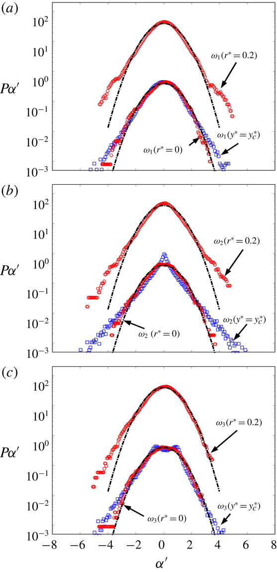
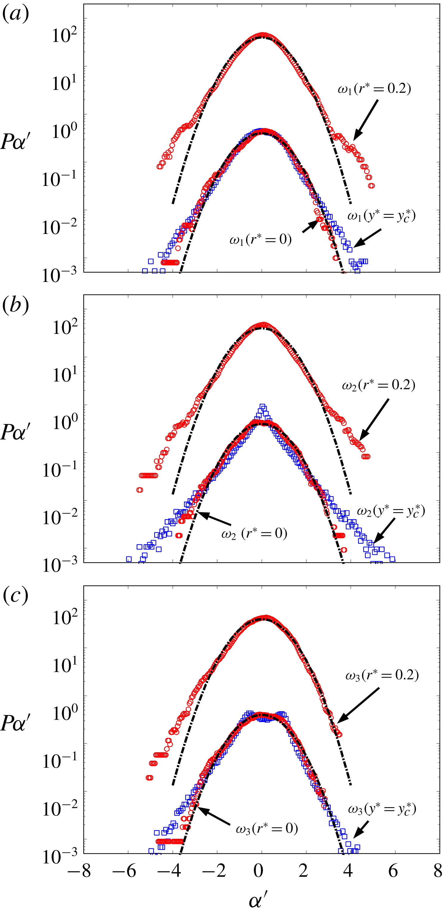
It is clearly of interest to also examine the p.d.f.s of the three components of the vorticity within the Kármán vortex. As expected, the conventional p.d.f.s $P_{\unicode[STIX]{x1D714}i}$ ( $i=1$ , 2 and 3) of the vorticity components at $y^{\ast }=y_{c}^{\ast }$ exhibit extended exponential tails (figure 8), reflecting the intermittency of the small-scale velocity field (e.g. She, Jackson & Orszag Reference She, Jackson and Orszag1991; Jiménez et al. Reference Jiménez, Wray, Saffman and Rogallo1993; Shafi & Antonia Reference Shafi and Antonia1997). Note that the conventional p.d.f.s of the three vorticity components also show different characteristics from each other, particularly around the peak of the p.d.f. Apparently, $P_{\unicode[STIX]{x1D714}_{2}}$ displays a more pronounced peak and more stretched tails than $P_{\unicode[STIX]{x1D714}_{1}}$ and $P_{\unicode[STIX]{x1D714}_{3}}$ , suggesting that $\unicode[STIX]{x1D714}_{2}$ is more intermittent than $\unicode[STIX]{x1D714}_{1}$ and $\unicode[STIX]{x1D714}_{3}$ in the present flow. This is corroborated by the larger kurtosis (not shown) of $\unicode[STIX]{x1D714}_{2}$ than those of $\unicode[STIX]{x1D714}_{1}$ and $\unicode[STIX]{x1D714}_{3}$ across the flow. The two peaks in $P_{\unicode[STIX]{x1D714}_{3}}$ which are opposite in sign are caused by the alternate arrangement of positive and negative vortices (figure 2 a). Like $P_{\unicode[STIX]{x1D703},i(r^{\ast }=0)}$ (figure 7), the p.d.f.s $P_{\unicode[STIX]{x1D714}_{i}(r^{\ast }=0)}$ of the three vorticity components at the vortex centre also tend to follow the Gaussian distribution better than their conventional p.d.f.s $P_{\unicode[STIX]{x1D714}_{i}(y^{\ast }=y_{c}^{\ast })}$ . However, at $r^{\ast }=0.2$ , the vorticity p.d.f.s exhibit an appreciable deviation from the Gaussian distribution, showing extended exponential tails. This is different from the scenario of the p.d.f.s of the velocities (figure 4 b–d) which follow the Gaussian distribution rather well at $r^{\ast }=0.2$ . This difference between the p.d.f.s of the vorticities and velocities resembles that between the p.d.f.s of the temperature derivatives and the temperature fluctuation. This is fully consistent with previous findings that the small-scale turbulence, irrespectively of whether the focus is on the velocity or temperature field, is more intermittent, resulting in the deviation of the corresponding p.d.f.s from the Gaussian distribution. The present result indicates that the Gaussian distribution is a good approximation of the small scales of the passive scalar and velocity fields only closely around the vortex centre within the vortex inner core region.

Figure 8.

Comparison between the p.d.f.s of the three components of the vorticity at different distances ( $r^{\ast }=0$ and 0.2) from the vortex centre and the Gaussian distribution. The conventional p.d.f.s at the same lateral position of the vortex centre are also included. The dash-dotted lines are Gaussian distribution.

Figure 9.

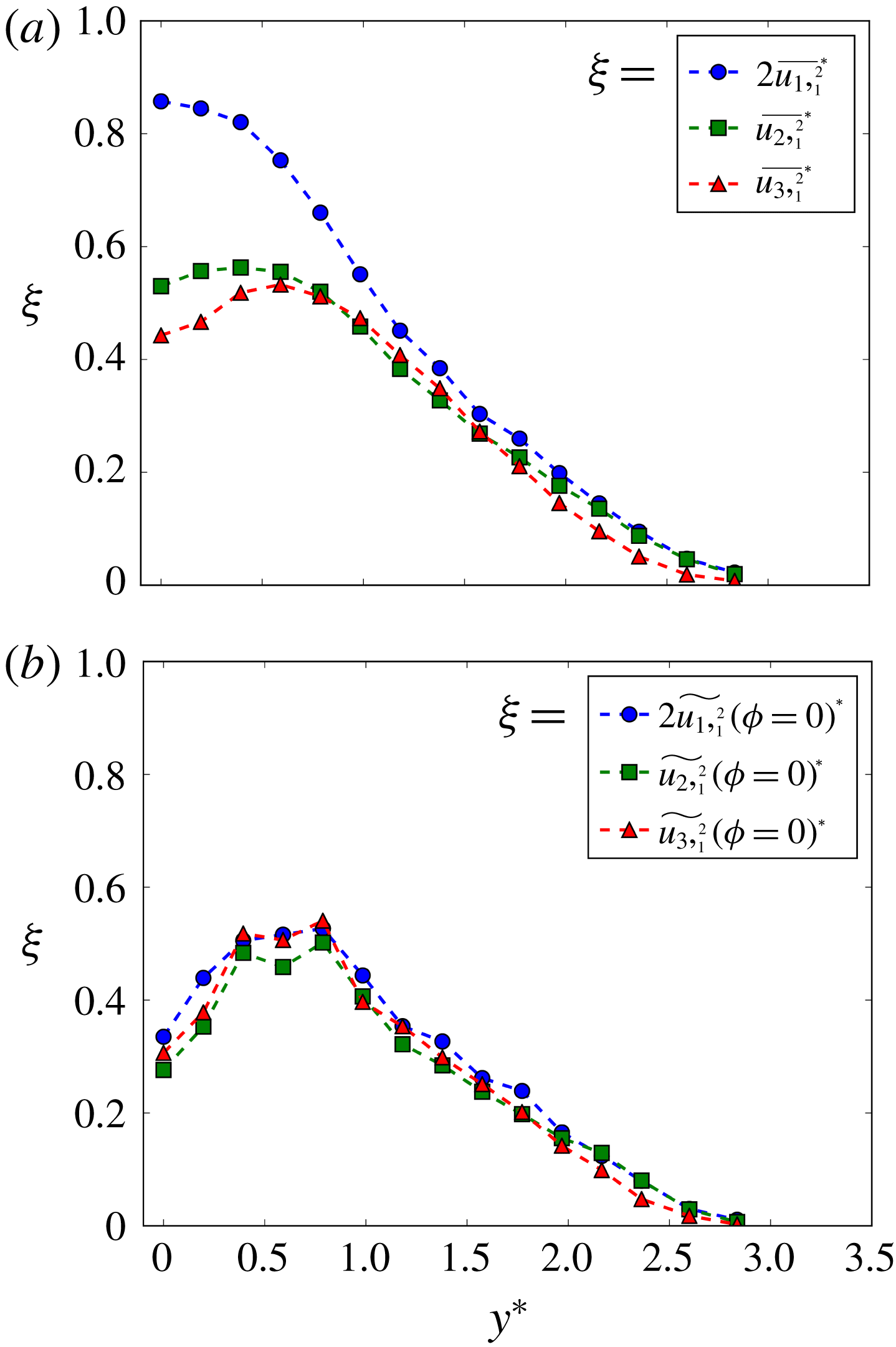
Comparison between the lateral distributions of the (a) conventional and (b) phase-averaged ( $\unicode[STIX]{x1D719}=0$ ) mean-square values of the streamwise derivative of the velocities.

Due to the inadequate spatial resolution of the probe, the value of the skewness and kurtosis of $\unicode[STIX]{x1D703}_{,i}$ and $\unicode[STIX]{x1D714}_{i}$ may not be completely trustworthy. Nevertheless, one can immediately infer from the closeness of the three p.d.f.s $P_{\unicode[STIX]{x1D703}_{,i}(r^{\ast }=0)}$ and $P_{\unicode[STIX]{x1D714}_{i}(r^{\ast }=0)}$ in figures 7 and 8 that the small scales around the vortex centre are not only Gaussian but also satisfy local isotropy approximately. Indeed, we estimate that the skewness and kurtosis of $\unicode[STIX]{x1D703}_{,i}$ and $\unicode[STIX]{x1D714}_{i}$ at the vortex centre are much closer to those of the Gaussian distribution than the corresponding statistics outside the vortex at the saddle point ( $\unicode[STIX]{x1D719}=\unicode[STIX]{x03C0}$ , $y^{\ast }=1.4$ , see figure 2). For example, the values of $|S|$ for ( $\unicode[STIX]{x1D703}_{,1}$ , $\unicode[STIX]{x1D703}_{,2}$ , $\unicode[STIX]{x1D703}_{,3}$ ) and ( $\unicode[STIX]{x1D714}_{1}$ , $\unicode[STIX]{x1D714}_{2}$ , $\unicode[STIX]{x1D714}_{3}$ ) at the vortex centre are (0.17, 0.27, 0.19) and (0.10, 0.12, 0.34), respectively, while those at the saddle point are (0.88, 1.73, 0.32) and (0.29, 0.21, 0.64), respectively. It is worth pointing out that it is extremely difficult to find a flow, including grid turbulence (see for example Antonia et al. Reference Antonia, Chambers, Van Atta, Friehe and Helland1978), where the skewness of the temperature derivative is zero. Also, $K$ of ( $\unicode[STIX]{x1D703}_{,1}$ , $\unicode[STIX]{x1D703}_{,2}$ , $\unicode[STIX]{x1D703}_{,3}$ ) and ( $\unicode[STIX]{x1D714}_{1}$ , $\unicode[STIX]{x1D714}_{2}$ , $\unicode[STIX]{x1D714}_{3}$ ) at the vortex centre are (4.6, 3.7, 3.6) and (4.2, 3.6, 3.5) respectively, while the corresponding $K$ at the saddle point are (13, 17, 15) and (9.0, 12, 7.6) respectively. The much higher kurtosis of $\unicode[STIX]{x1D703}_{,i}$ and $\unicode[STIX]{x1D714}_{i}$ at the saddle point also indicates that the high intermittency in the conventional p.d.f.s of $\unicode[STIX]{x1D703}_{,i}$ and $\unicode[STIX]{x1D714}_{i}$ (figures 7 and 8) is largely due to the contribution of the flow field outside the vortex in the saddle region.

In view of the smaller values of $|S|$ of $\unicode[STIX]{x1D703}_{,i}$ and $\unicode[STIX]{x1D714}_{i}$ at the vortex centre, one can expect the flow field in the vortex core region to be more locally isotropic, compared to the conventionally averaged flow. For locally isotropic turbulence, the following equations should be satisfied (Taylor Reference Taylor1935)

(4.1) $$\begin{eqnarray}\displaystyle & \overline{{u_{1,}}_{1}^{2}}=\overline{{u_{2,}}_{2}^{2}}=\overline{{u_{3,}}_{3}^{2}}, & \displaystyle\end{eqnarray}$$

(4.2) $$\begin{eqnarray}\displaystyle & 2\overline{{u_{1,}}_{1}^{2}}=\overline{{u_{1,}}_{2}^{2}}=\overline{{u_{1,}}_{3}^{2}}=\overline{{u_{2,}}_{1}^{2}}=\overline{{u_{2,}}_{3}^{2}}=\overline{{u_{3,}}_{1}^{2}}=\overline{{u_{3,}}_{2}^{2}}, & \displaystyle\end{eqnarray}$$

and

(4.3) $$\begin{eqnarray}\overline{u_{1,2}u_{2,1}}=\overline{u_{1,3}u_{3,1}}=\overline{u_{2,3}u_{3,2}}=-1/2\overline{u_{1,1}^{2}}.\end{eqnarray}$$

For a locally isotropic temperature field, the different components $\overline{\unicode[STIX]{x1D703},_{i}^{2}}$ ( $i=1$ , 2 and 3) of the temperature dissipation rate must be equal to each other (e.g. Sreenivasan Reference Sreenivasan1991). Because $\overline{\unicode[STIX]{x1D703},_{2}^{2}}$ and $\overline{\unicode[STIX]{x1D703},_{3}^{2}}$ would be attenuated due to the inadequate spatial resolution of the probe in the $y$ and $z$ directions (please refer to the earlier discussion of the probe resolution), a simplified test of local isotropy for the velocity field within the Kármán vortex is made here by checking whether the equations in (4.2) associated with $u_{i,1}$ ( $i=1$ , 2, 3) are satisfied within the vortex. Note that the spatial resolution of the probe in the streamwise direction is $5.8\unicode[STIX]{x1D702}$ , quite close to the optimum resolution range ( $3{-}5\unicode[STIX]{x1D702}$ ). 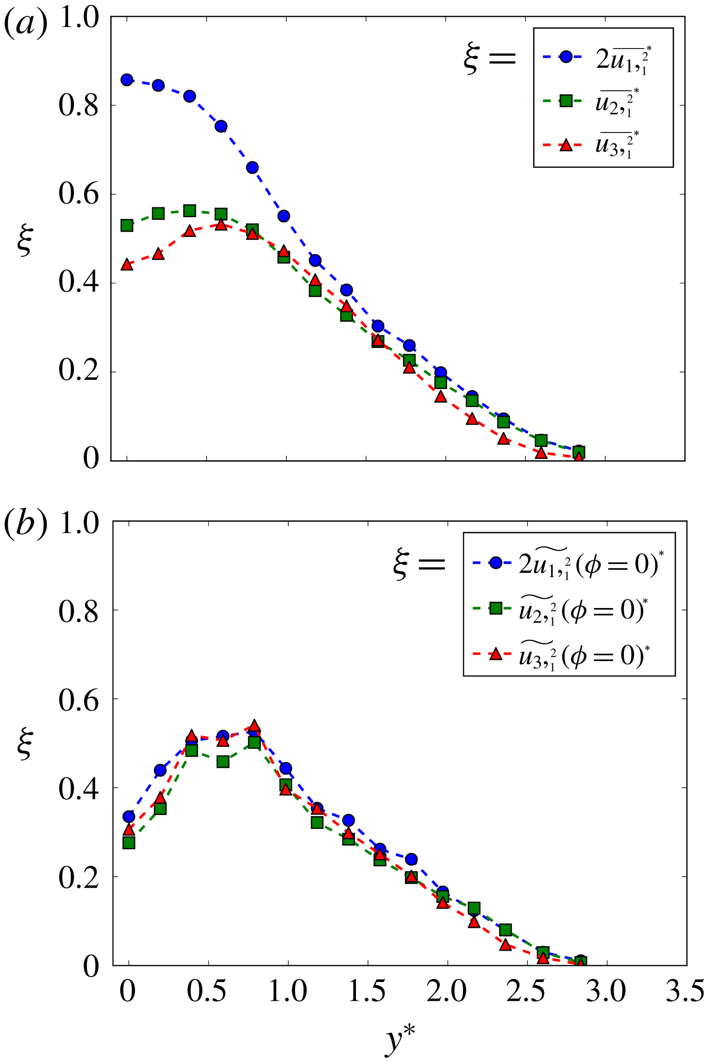Thus, the attenuation of the mean-square velocity derivatives should be minimum in the streamwise direction. Figure 9 exhibits the distributions of the mean-square value of $u_{i,1}$ within the Kármán vortex at the same phase as the vortex centre ( $\unicode[STIX]{x1D719}=0$ ), and those of the conventional mean-square values. The conventional distributions of $2\overline{u_{1},_{1}^{2}}^{\ast }$ , $\overline{u_{2},_{1}^{2}}^{\ast }$ and $\overline{u_{3},_{1}^{2}}^{\ast }$ deviate appreciably from each other (figure 9 a), particularly at $y^{\ast }<1$ . This is not unexpected because the coherent motions, including the spanwise Kármán vortices and the streamwise ribs, in the near wake are strongly anisotropic. This departure between the mean-square velocity derivatives, which decreases downstream, is not negligible even in the self-preserving far wake (e.g. Browne, Antonia & Shah Reference Browne, Antonia and Shah1987). However, the distributions of $2\widetilde{u_{1},_{1}^{2}}(\unicode[STIX]{x1D719}=0)^{\ast }$ , $\widetilde{u_{2},_{1}^{2}}(\unicode[STIX]{x1D719}=0)^{\ast }$ and $\widetilde{u_{3},_{1}^{2}}(\unicode[STIX]{x1D719}=0)^{\ast }$ are close to each other (figure 9 b), which is fully consistent with (4.2). The peak of the mean-square values occurs in the region $y^{\ast }=0.4{-}0.8$ in figure 9(a), which corresponds to the $y^{\ast }$ range where the vortex core region resides (figure 2 a). It may be inferred that the turbulent energy dissipation rate ( $\equiv \unicode[STIX]{x1D708}\overline{u_{i,j}(u_{i,j}+u_{j,i})}$ , which can be simplified as $15\unicode[STIX]{x1D708}\overline{u_{1},_{1}^{2}}$ for isotropic turbulence) within the vortex will have its maximum value in the same $y^{\ast }$ range (i.e. 0.4–0.8). This is confirmed by the spatial distribution of the turbulent energy dissipation rate in the same flow (see figure 11 of Chen et al. Reference Chen, Zhou, Antonia and Zhou2018).

5 Physical difference within and outside the vortex

The statistics within the Kármán vortex of the temperature and velocity fields, including both fluctuations $u_{i}$ and $\unicode[STIX]{x1D703}$ (§ 3) and small scales $\unicode[STIX]{x1D714}_{i}$ and $\unicode[STIX]{x1D703}_{,i}$ (§ 4) are quite different from their conventional counterparts, especially within the inner core region. Their contrasting behaviours, shown in figures 4–8, indicate that the physics is different inside and outside the vortex.

The spanwise vortex rolls and the streamwise ribs are the predominant coherent structures in the near wake. The former induces the fluctuating velocities $u_{1}$ and $u_{2}$ , while the latter is the major contributor to $u_{3}$ (e.g. Djenidi & Antonia Reference Djenidi and Antonia2009). The presence of the cool fluid entrained by the vortex rolls from the free stream results in the occurrence of large-scale temperature fronts outside the vortex. The coherent strain between the consecutive vortices accounts for the temperature front near the saddle point aligned along the diverging separatrix (e.g. Antonia et al. Reference Antonia, Chambers, Britz and Browne1986; Matsumura & Antonia Reference Matsumura and Antonia1993; also figure 2 b). In distinct contrast to the complex structures outside the Kármán vortex, the flow field within the vortex is filled with random incoherent motions (Hussain & Hayakawa Reference Hussain and Hayakawa1987) and the highly concentrated temperature fluctuations of warm fluid (Matsumura & Antonia Reference Matsumura and Antonia1993). The flow region within the inner vortex core is essentially ‘sheltered’ from the various coherent motions outside the vortex. Therefore, the nearly Gaussian distributions of the fluctuations $u_{i}(r^{\ast })$ and $\unicode[STIX]{x1D703}_{i}(r^{\ast })$ around the vortex centre are not unexpected. This is also why the p.d.f.s of $u_{i}(r^{\ast })$ and $\unicode[STIX]{x1D703}_{i}(r^{\ast })$ gradually depart from the Gaussian distribution with increasing $r^{\ast }$ (figure 4). Note that the p.d.f. of $u_{2}(r^{\ast }=0.6)$ (figure 4 c) tends to exhibit two peaks similar to those observed in $P_{u_{2}(y^{\ast }=y_{c}^{\ast })}$ . This is essentially a footprint of the positive and negative coherent $u_{2}$ induced by the Kármán vortex on either side of its centroid.

The large-scale structures outside the vortex are also expected to influence $\unicode[STIX]{x1D714}_{i}$ and $\unicode[STIX]{x1D703}_{,i}$ . Two factors account for the high intermittency of $\unicode[STIX]{x1D714}_{i}$ and $\unicode[STIX]{x1D703}_{,i}$ outside the vortex, as reflected by the stretched tails and/or a spiky peak in the conventional p.d.f.s of $\unicode[STIX]{x1D703}_{,i}$ (figure 7) and $\unicode[STIX]{x1D714}_{i}$ (figure 8). Firstly, irrotational fluid is entrained from the free stream (figure 2 b), resulting in the concentrated patches of $\unicode[STIX]{x1D714}_{i}$ and $\unicode[STIX]{x1D703}_{,i}$ interspersed with quieter regions of irrotational fluid. This is often referred to as external intermittency (Cossin Reference Cossin1943; Davidson Reference Davidson2015, p. 377). Secondly, the vortex stretching caused by the coherent strain in the saddle region produces fine-scale turbulent fluctuations. As such, the large and small scales of both temperature and velocity fields could be coupled at the saddle region. This effect of the large scales on the small scales of the turbulence can also lead to the high intermittency of the small scales (Landau & Lifschitz Reference Landau and Lifschitz1987). In contrast, one may surmise that the coupling between large and small scales of the fluctuating temperature or velocity field is rather weak around the vortex centre, which would account for the observation that the p.d.f.s of the temperature derivative and the vorticity are quite close to the Gaussian distribution. To gain some further sight into this, we take two approaches to evaluate the degree of coupling between the large and small scales of both temperature and velocity fields within and outside the vortex.

Figure 10.

Colour-filled iso-contours of the correlation coefficients at the same phase $\unicode[STIX]{x1D70C}(\unicode[STIX]{x1D713},\unicode[STIX]{x1D701}|\unicode[STIX]{x1D719})$ : (a) $\unicode[STIX]{x1D713}=\unicode[STIX]{x1D703}$ and $\unicode[STIX]{x1D701}=\unicode[STIX]{x1D712}$ , (b) $\unicode[STIX]{x1D713}=q$ and $\unicode[STIX]{x1D701}=\unicode[STIX]{x1D714}^{2}$ . The iso-contours of $\unicode[STIX]{x1D703}$ (solid lines represent positive $\unicode[STIX]{x1D703}$ and dashed lines are for negative $\unicode[STIX]{x1D703}$ ) are superposed in (a) for reference.

The first is the phase-averaged correlation coefficient defined by

(5.1) $$\begin{eqnarray}\unicode[STIX]{x1D70C}(\unicode[STIX]{x1D713},\unicode[STIX]{x1D701}|\unicode[STIX]{x1D719})\equiv \left[\left.\frac{\overline{(\unicode[STIX]{x1D713}-E(\unicode[STIX]{x1D713}))(\unicode[STIX]{x1D701}-E(\unicode[STIX]{x1D701}))}}{\unicode[STIX]{x1D70E}_{\unicode[STIX]{x1D713}}\unicode[STIX]{x1D70E}_{\unicode[STIX]{x1D701}}}\right|\unicode[STIX]{x1D719}\right],\end{eqnarray}$$

where $\unicode[STIX]{x1D713}$ stands for $\unicode[STIX]{x1D703}$ or the turbulent kinetic energy $q$ ( $\equiv u_{1}^{2}+u_{2}^{2}+u_{3}^{2}$ ), representing the large scales in the temperature or velocity field, and $\unicode[STIX]{x1D701}$ stands for the temperature dissipation rate $\unicode[STIX]{x1D712}$ ( $\equiv \unicode[STIX]{x1D703}_{,1}^{2}+\unicode[STIX]{x1D703}_{,2}^{2}+\unicode[STIX]{x1D703}_{,3}^{2}$ ) or enstrophy $\unicode[STIX]{x1D714}^{2}$ ( $\equiv \unicode[STIX]{x1D714}_{1}^{2}+\unicode[STIX]{x1D714}_{2}^{2}+\unicode[STIX]{x1D714}_{3}^{2}$ ), which characterizes the small scales. The $\unicode[STIX]{x1D70C}(\unicode[STIX]{x1D713},\unicode[STIX]{x1D701}|\unicode[STIX]{x1D719})$ quantifies the correlation between the large scales and small scales of the temperature or velocity field at the same phase. It should be noted that, at a given phase $\unicode[STIX]{x1D719}$ , $E(\unicode[STIX]{x1D713})$ and $E(\unicode[STIX]{x1D701})$ are not necessarily 0, but equal to their corresponding phase-averaged values at this phase, i.e. $\widetilde{\unicode[STIX]{x1D713}}(\unicode[STIX]{x1D719})$ and $\widetilde{\unicode[STIX]{x1D701}}(\unicode[STIX]{x1D719})$ . Technically, $\unicode[STIX]{x1D70C}(\unicode[STIX]{x1D703}^{2},\unicode[STIX]{x1D712}|\unicode[STIX]{x1D719})$ is more analogous to $\unicode[STIX]{x1D70C}(q,\unicode[STIX]{x1D714}^{2}|\unicode[STIX]{x1D719})$ than $\unicode[STIX]{x1D70C}(\unicode[STIX]{x1D703},\unicode[STIX]{x1D712}|\unicode[STIX]{x1D719})$ . But here we would like to highlight the effect of the temperature front (interface between positive and negative temperature) on the coupling between distinct scales in the temperature field. Therefore, $\unicode[STIX]{x1D70C}(\unicode[STIX]{x1D703},\unicode[STIX]{x1D712}|\unicode[STIX]{x1D719})$ is employed to avoid the ambiguity of the temperature front caused by $\unicode[STIX]{x1D703}^{2}$ .

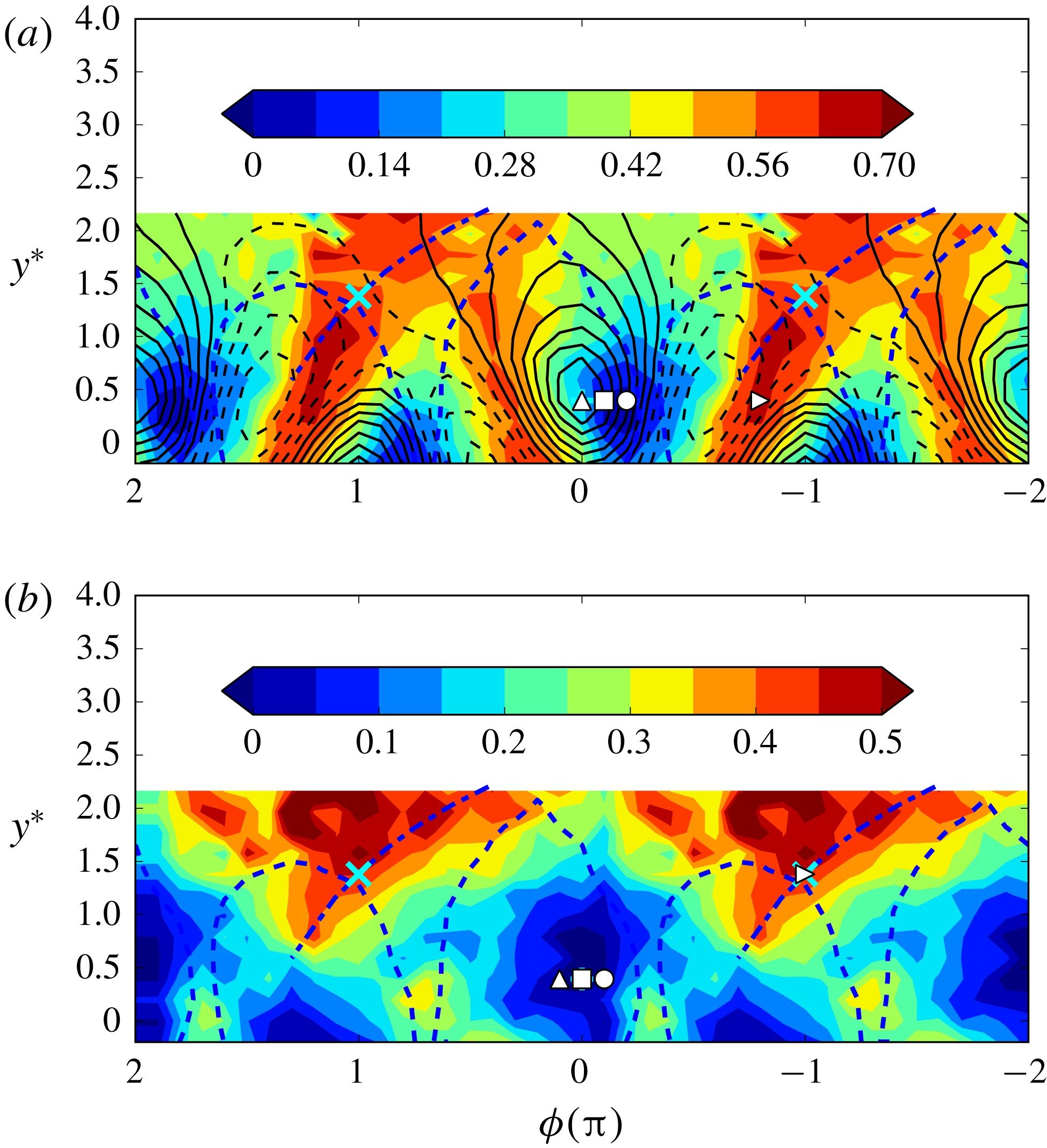
Figure 10(a) shows the iso-contours of $\unicode[STIX]{x1D70C}(\unicode[STIX]{x1D703},\unicode[STIX]{x1D712}|\unicode[STIX]{x1D719})$ , superposed onto the iso-contours of the phase-averaged temperature (figure 2 b) which serve as a reference. A large value of $\unicode[STIX]{x1D70C}(\unicode[STIX]{x1D703},\unicode[STIX]{x1D712}|\unicode[STIX]{x1D719})$ , of the order of 0.7, appears in the saddle region along the diverging separatrix where the large-scale temperature front forms, while a much smaller value, close to 0, is associated with the downstream half of the vortex. The minimum correlation coefficient does not occur at the vortex centre, probably because of the physical separation between the concentrations of $\unicode[STIX]{x1D703}$ and $\unicode[STIX]{x1D712}$ within the vortex. It is noted that the presence of the entrained cool fluid in the warm wake gives rise to two large-scale cool–warm temperature fronts, one near the saddle point and aligned along the diverging separatrix and the other immediately downstream of the vortex (figure 2 b). The former is associated with large $\unicode[STIX]{x1D70C}(\unicode[STIX]{x1D703},\unicode[STIX]{x1D712}|\unicode[STIX]{x1D719})$ , while the latter is related to small $\unicode[STIX]{x1D70C}(\unicode[STIX]{x1D703},\unicode[STIX]{x1D712}|\unicode[STIX]{x1D719})$ (figure 10 a). The observation suggests that the magnitude of the coherent strain in the saddle region plays a crucial role in the interaction between different scales in the temperature field. This is presumably because the strain rate may act to amplify the temperature gradient (e.g. Pumir Reference Pumir1994). The large values of $\unicode[STIX]{x1D70C}(q,\unicode[STIX]{x1D714}^{2}|\unicode[STIX]{x1D719})$ , of the order of 0.5, occur in the saddle region, while near-zero magnitudes of $\unicode[STIX]{x1D70C}(q,\unicode[STIX]{x1D714}^{2}|\unicode[STIX]{x1D719})$ reside around the centre of the Kármán vortex (figure 10 b). It may be inferred from figure 10(a,b) that the large and small scales of both velocity and temperature fields are, at best, loosely coupled within the Kármán vortex but are strongly coupled outside, especially in the saddle region under the effect of the coherent strain.

Another way of evaluating the degree of coupling between the large and small scales is to examine the expectation of $\unicode[STIX]{x1D714}^{2}$ conditioned on $q$ and that of $\unicode[STIX]{x1D712}$ conditioned on $\unicode[STIX]{x1D703}$ at different locations in the flow. One may expect that the dependence between $\unicode[STIX]{x1D703}$ and $\unicode[STIX]{x1D712}$ , or $q$ and $\unicode[STIX]{x1D714}^{2}$ , is weak in a region where their correlation coefficient is small. The dependence of $\unicode[STIX]{x1D712}$ on $\unicode[STIX]{x1D703}$ and $\unicode[STIX]{x1D714}^{2}$ on $q$ may be given by the conditional expectations of $\unicode[STIX]{x1D712}(\unicode[STIX]{x1D719})$ and $\unicode[STIX]{x1D714}^{2}(\unicode[STIX]{x1D719})$ , i.e. 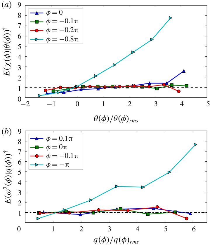$E(\unicode[STIX]{x1D712}(\unicode[STIX]{x1D719})|\unicode[STIX]{x1D703}(\unicode[STIX]{x1D719}))^{\dagger }$ and $E(\unicode[STIX]{x1D714}^{2}(\unicode[STIX]{x1D719})|q(\unicode[STIX]{x1D719}))^{\dagger }$ , where ‘ $\dagger$ ’ denotes normalization by $\widetilde{\unicode[STIX]{x1D712}}(\unicode[STIX]{x1D719})$ and $\widetilde{\unicode[STIX]{x1D714}^{2}}(\unicode[STIX]{x1D719})$ , respectively. A few typical locations are marked in figure 10(a). A constant $E(\unicode[STIX]{x1D712}(\unicode[STIX]{x1D719})|\unicode[STIX]{x1D703}(\unicode[STIX]{x1D719}))^{\dagger }$ is expected when $\unicode[STIX]{x1D712}(\unicode[STIX]{x1D719})$ and $\unicode[STIX]{x1D703}(\unicode[STIX]{x1D719})$ are statistically independent of each other. For locations associated with a small correlation coefficient, i.e. $\unicode[STIX]{x1D719}=0$ , $-0.1\unicode[STIX]{x03C0}$ and $-0.2\unicode[STIX]{x03C0}$ , $E(\unicode[STIX]{x1D712}(\unicode[STIX]{x1D719})|\unicode[STIX]{x1D703}(\unicode[STIX]{x1D719}))^{\dagger }$ (figure 11 a) is generally equal to unity at different $\unicode[STIX]{x1D703}(\unicode[STIX]{x1D719})$ , indicating that $\unicode[STIX]{x1D712}(\unicode[STIX]{x1D719})$ is statistically independent of $\unicode[STIX]{x1D703}(\unicode[STIX]{x1D719})$ at these locations. In contrast, $E(\unicode[STIX]{x1D712}(\unicode[STIX]{x1D719})|\unicode[STIX]{x1D703}(\unicode[STIX]{x1D719}))^{\dagger }$ exhibits a significant dependence on $\unicode[STIX]{x1D703}(\unicode[STIX]{x1D719})$ when $\unicode[STIX]{x1D70C}(\unicode[STIX]{x1D703},\unicode[STIX]{x1D712}|\unicode[STIX]{x1D719})$ is large at $\unicode[STIX]{x1D719}=-0.8\unicode[STIX]{x03C0}$ . At this position, a large value of $E(\unicode[STIX]{x1D712}(\unicode[STIX]{x1D719})|\unicode[STIX]{x1D703}(\unicode[STIX]{x1D719}))^{\dagger }$ is associated with a large magnitude of $\unicode[STIX]{x1D703}(\unicode[STIX]{x1D719})$ . A similar scenario applies for the dependence of $\unicode[STIX]{x1D714}^{2}$ on $q$ (figure 11 b). For phases $\unicode[STIX]{x1D719}=0.1$ , 0, $-0.1\unicode[STIX]{x03C0}$ where $\unicode[STIX]{x1D70C}(q,\unicode[STIX]{x1D714}^{2}|\unicode[STIX]{x1D719})$ is small (figure 11 b), $E(\unicode[STIX]{x1D714}^{2}(\unicode[STIX]{x1D719})|q(\unicode[STIX]{x1D719}))^{\dagger }$ is essentially equal to unity. On the other hand, at $\unicode[STIX]{x1D719}=-\unicode[STIX]{x03C0}$ where $\unicode[STIX]{x1D70C}(q,\unicode[STIX]{x1D714}^{2}|\unicode[STIX]{x1D719})$ is large (figure 11 b), $E(\unicode[STIX]{x1D714}^{2}(\unicode[STIX]{x1D719})|q(\unicode[STIX]{x1D719}))^{\dagger }$ deviates from unity and increases with the value of  $q$ .

Figure 11.

Conditional expectations (a) $E(\unicode[STIX]{x1D712}(\unicode[STIX]{x1D719})|\unicode[STIX]{x1D703}(\unicode[STIX]{x1D719}))^{\dagger }$ and (b) $E(\unicode[STIX]{x1D714}^{2}(\unicode[STIX]{x1D719})|q(\unicode[STIX]{x1D719}))^{\dagger }$ at four spatial locations marked in figures 10(a) and 10(b), respectively.

In summary, figures 10 and 11 show unequivocally a marked difference within and outside the Kármán vortex in the interaction between the large- and small-scale structures. This result conforms with the perception that the coherent strain in the saddle region plays an important role in this interaction. It confirms our assertion that the flow field within the vortex core region is ‘sheltered’ from the effect of the large-scale structures or coherent strain outside, resulting in the Gaussian p.d.f.s of fluctuating velocities and temperature within this region.

6 Conclusions and further discussion

We have investigated the velocity and temperature fields within the Kármán vortex generated by a circular cylinder using phase averaging. To our knowledge, this is the first time when the statistics of both the velocity and temperature or passive scalar fields within the Kármán vortex have been presented in such detail. The following conclusions can be drawn.

(i) The turbulent Kármán vortex is characterized by a rapid and approximately linear rise in the tangential velocity $\widetilde{u_{2}}(r_{1})^{\ast }$ within the inner core region ( $r_{1}^{\ast }\leqslant r_{c}^{\ast }$ ) of the vortex. The temperature and velocity fields within the Kármán vortex display quite different statistical features from their corresponding conventional statistics. The p.d.f.s of the fluctuating temperature and velocities within the inner core region exhibit essentially a Gaussian distribution. In contrast, their corresponding conventional p.d.f.s, especially the p.d.f.s of $u_{2}$ and $\unicode[STIX]{x1D703}$ , depart noticeably from the Gaussian distribution due to the presence of strong coherent motions or the cool fluid entrained by these motions. The distributions of $\widetilde{u_{1}^{2}}(r_{1})^{\ast }$ and $\widetilde{u_{3}^{2}}(r_{1})^{\ast }$ have a minimum at the vortex centre and rise to their maximum at $r_{1}^{\ast }=r_{c}^{\ast }$ . The distribution of $\widetilde{\unicode[STIX]{x1D703}^{2}}(r_{1})^{\ast }$ remains unchanged at its largest magnitude within the inner core region. The observations suggest that the flow behaviour within $r^{\ast }\leqslant r_{c}^{\ast }$ is quite different from that in the region $r^{\ast }>r_{c}^{\ast }$ . The p.d.f.s of $u_{i}$ and $\unicode[STIX]{x1D703}$ follow the Gaussian distribution closely within the inner core region, but not outside. It is found that the warm fluid boundary within the vortex ( $\widetilde{\unicode[STIX]{x1D703}}(r_{1})^{\ast }=0$ ) corresponds approximately to the outer core radius ( $r_{o}^{\ast }$ ) where $\widetilde{u_{2}}(r_{1})^{\ast }$ reaches its maximum value. The finding suggests that it is the strong rotational motion of the vortex that is responsible for retaining the heat within the vortex. Based on this finding, one may surmise that the tornado-like vortex may be also characterized by two critical radii, i.e. $r_{c}^{\ast }$ and $r_{o}^{\ast }$ , although the former one is not recognized in the studies of the tornado vortex (e.g. Hu et al. Reference Hu, Yang, Sarkar and Haan2011; Yang, Sarkar & Hu Reference Yang, Sarkar and Hu2011).

(ii) The p.d.f.s of the components of the temperature gradient and vorticity follow closely the Gaussian distribution at the vortex centre but their conventional counterparts do not. Away from the vortex centre, say at $r^{\ast }=0.2$ , the p.d.f.s of the vorticities and the temperature derivatives deviate from the Gaussian distribution. The region where the p.d.f.s of the temperature derivative and vorticity fluctuations can be approximated by a Gaussian distribution is smaller than that for temperature and velocity fluctuations.

(iii) The distinct interactions between the large- and small-scale structures within and outside the vortex underpin the corresponding different behaviours of the statistics of the temperature and velocity fields. The behaviour of the phase-averaged correlation coefficients $\unicode[STIX]{x1D70C}(\unicode[STIX]{x1D703},\unicode[STIX]{x1D712}|\unicode[STIX]{x1D719})$ and $\unicode[STIX]{x1D70C}(q,\unicode[STIX]{x1D714}^{2}|\unicode[STIX]{x1D719})$ suggests that small-scale structures within the vortex feel little effect from the large scales. On the other hand, the large- and small-scale structures are strongly coupled outside the vortex, especially in the saddle region, for both velocity and temperature fields. The strong coherent strain in the saddle region provides a strong link between the large- and small-scale structures. This is further substantiated by the marked difference in the conditional expectations $E(\unicode[STIX]{x1D712}(\unicode[STIX]{x1D719})|\unicode[STIX]{x1D703}(\unicode[STIX]{x1D719}))^{\dagger }$ and $E(\unicode[STIX]{x1D714}^{2}(\unicode[STIX]{x1D719})|q(\unicode[STIX]{x1D719}))^{\dagger }$ within and outside the vortex, which correspond to small and large conditional correlation coefficients, respectively.

The present study indicates that the turbulence within the inner core of the vortex centre is very close to being homogeneous and locally isotropic (figure 9). Kolmogorov (Reference Kolmogorov1941) assumes the hypothesis of local isotropy is realized with good approximation in sufficiently small domains when the Reynolds number is adequately large. The present findings suggest that the Reynolds number may not need to be extremely large ( $Re_{\unicode[STIX]{x1D706}}$ is approximately 110 at the vortex centre) to achieve approximately locally isotropic turbulence, as long as the effect of the large scales can be avoided. This is in full accord with the findings of Antonia, Djenidi & Danaila (Reference Antonia, Djenidi and Danaila2014) that the Kolmogorov scaling applies only when the large-scale term in the transport equations for the second-order velocity structure function can be neglected. The Gaussian p.d.f. of the temperature inside the vortex inner core suggests that the passive scalar has been sufficiently mixed in this region. This raises a number of interesting issues which should be worth pursuing in future studies, preferably with the use of direct numerical simulation (DNS). The first relates to the process and mechanisms by which the temperature becomes well mixed inside the vortex. One expects the temperature to have non-Gaussian characteristics within the boundary layer over the heated surface of the cylinder. Following separation, the thermal shear layer is subjected to large fluctuating strain rates and indeed the small-scale temperature fluctuations are highly intermittent and non-Gaussian in the region near the saddle point. Nonetheless, the heated fluid that is transported into the core of the vortex and subjected vigorously to the rotational motion within the vortex is remarkably close to being Gaussian and locally isotropic. DNS should allow a reliable estimation of the energy (and scalar variance) budgets within the vortex and therefore lead to useful information on the scale-by-scale energy and scalar variance budgets within the vortex. This, in turn, should provide important insight into why the small-scale statistics in the vortex core are seemingly unaffected by the large scales of the flow. Finally, the Gaussian nature of the small-scale fluctuations in the vortex core should make it attractive to estimate statistics of pressure fluctuation in the core using the joint-Gaussian calculation of Batchelor (Reference Batchelor1951), see also Pearson & Antonia (Reference Pearson and Antonia2001); these statistics should of course be compared with those estimated directly from DNS.