Introduction

Variations in sea-ice pressure ridging reflect the different dynamics of the pack ice. in turn, the ridges can alter the momentum transfer between the sea ice, atmosphere and ocean (Reference Andreas, Lange, Ackley and WadhamsAndreas and others, 1993). The ice-thickness distribution can be used to estimate the salt flux to the ocean and the ocean/atmosphere heal transfer (Reference Maykut and UntersteinerMaykut, 1986). The amount of sea ice contained within ridges may comprise a significant fraction of the total ice volume. Several studies (e.g. Reference Allison and WorbyAllison and Worby, 1994; Worby and others, 1996a, 1998) have used ship-based observations to estimate the volume of ice contained in ridges. They find that the ice thickness and ridging intensity may decrease significantly near the coast due to the rapid offshore transport of ice by katabatic winds. Worby and others (1998) estimate that in the East Antarctic region, ridging can account for 0.36 m, or 42%, of the area-averaged thickness, based on a mean areal coverage of 11 %. Other studies of ridging of Antarctic-sea ice have used airborne laser altimeters (Reference Weeks, Ackley and GovoniWeeks and others, 1989; Dicrking, 1995), or acoustic altimeters operated from ships (Lytle and Acklcy, 1991). These studies found that sea-ice ridge intensity is usually higher by as much as an order of magnitude near the coast as compared with the interior pack. The divergent region observed by Allison and Worby (1994) may not have been present in these alti-meter studies, or the altimeter studies may not have measured the ice immediately adjacent to the coast.

We use aerial photography collected over sea ice during a field experiment in August 1995, near 65° S, 140° E, to estimate ridge heights and frequency. This region is characterised by a narrow band of highly mobile ice which rarely extends more than 500 km from the continent (Worby and others, 1998). The low SนN angles at this time of year (≤13°) cause long shadows to be cast by ridges, and the large contrast between the shadowed areas and white snow in the aerial images provides an effective way to measure ridge heights as small as 0.1m. Ridge statistics from the photographs are compared with ship-based observations,and synthetic aperture radar (SAR) to define regions with different ridge characteristics.

Data Collection and Processing

The aerial photographs used in this study were collected on 8, 9,16, 20 and 23 August 1995 using a digital camera mounted to look vertically downward through the floor of a helicopter. Flight altitudes ranged from approximately 1500 to 2400 m (5000-8000 ft), resulting in a ground resolution of 0.5-().8 m, respectively.The altitude was accurate to within about 70 m, resulting in a maximum error in the pixel size of 0.02 m. The photographs cover the latitudinal range 64.2-65.6°S, and provide accurate information on floe-size distribution, thin ice and open water concentration, and ridge statistics.

SAR data were collected in the region 64-66.5° S, 132 144° E by the European remote-sensing satellite ERS-1 on 2,5, 21 and 27 August and 2 September 1995. These data extend east and west of the photographs and ship-based observations. Ten SAR images collected from ERS-2 the following winter, on 6, 9 and 10 August 1996, were also analyzed. Although there are no in situ data for 1996, we use the limited SAR data to determine if the ice characteristics seen in 1995 are also present the following year. After calibrating (Latir, 1992) and gcolocating the images, we calculate the average backscatter (₀^ₒ) for each 18.5 km band (10 min) of latitude. The width of each band is determined by the width of the satellite swath. The SAR image from 2 August 1995 is shown in Figure 1. The open water fraction, determined from the ship-based observations and aerial

Fig. 1.

SAR image collected oversea ice on 2 August 1995. This is a composite of three different SAR frames, centred on about 140° E longitude. The SAR images are about 110km wide, and north is towards the top left. See text for discussion of the three regions. SAR image © European space Agency, 1995.

photography, was less than about 6% in the region 65.6-64.2°S. Therefore, with the exception of the large flaw lead along the fast ice to the south, ₀^ₒ should not be greatly influenced by wind roughening on open water patches. The ice edge, estimated from the SAR images on 2 August, was at about 62.4° S, approximately 200 km north of the image shown. Its position in the SAR images varied considerably, ranging between 60.5° and 62.5°S, throughout August 1995.

The ship travelled around the perimeter of the 110 km X 110 km study region three times during the 3 week experiment (Worby and others, 1996b). Hourly ship-based ice observations were collected, including an estimate of the areal extent of ridging. These observations were sorted by latitude, and 20 observations have been averaged to estimate the areal extent of ridging. This averaging removes any small-scale variations in ridging, and any time dependence between observations in the same region at different times.

Model

From the aerial photographs, we calculate the area-averaged ice thickness with in the ridges using two different methods: by calculating a ridge height distribution, and total ridged volume.

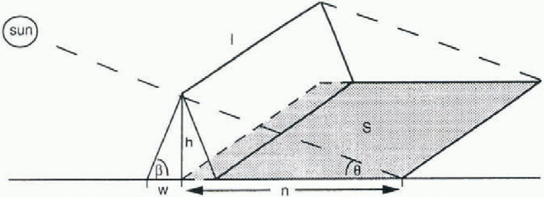
Ridge height distribution lb estimate a ridge height distribution, randomly spaced linear transects are drawn across the photograph. This mimics the linear transects measured by laser or acoustical devices to determine ridge height distributions in other studies (e.g. Reference DierkingDierking, 1995). Although these transects are randomly spaced, they are oriented in the direction of the SนN angle. The length of the intersection between the shadow and the transect is proportional to the height of the ridge, h, by:

(1)

where N is the length of the shadow in the photograph and δ is the SนN angle from the horizon (Fig. 2). Following Reference Hibler, Mock and TuckerHibler and others (1974), we compute the frequency of ridges, μ, the mean ridge height, (h), and the area-averaged volume per unit area of deformed ice contained in the ridges, pX, as:

(2)

where (h²) is the mean-squared ridge height and ß is the ridge slope. The subscript "x" denotes the minimum cut-off height used to determine (h²) and μ. This formulation assumes that the orientation of the ridges is random, and the ratio of the ice above and below the surface is 1:5. This ratio is based on studies by Worby and others (1998) of drilled ridge profiles of sea ice in East Antarctica. It is primarily affected by the average snow loading on the surface of the ice floe, β is taken as 25°, used by other researchers (e.g. Reference Tucker and GovoniTucker and Govoni, 1981; Dierking, 1995), and is near the average found byReference Timco and BurdenTimco and Burden (1997) for first-year ridges in the Arctic.

Fig. 2.

The triangular ridge geometry used in this study.

Total ridged volume

The volume of ridged ice is estimated from the total area of the photograph which is in shadow. We assume a triangular ridge geometry (Fig. 2) with height h, length I and half-width W (Tucker and Govoni, 1981). The area in the shadow of the photographs,5, can be related to the ridge height and length by:

(3)

where the factor π/2 accounts for the fact that the ridges are randomly aligned relative to the sun. For a constant ß, lh tan ß is a measure of the surface area covered by the

Table. 1.

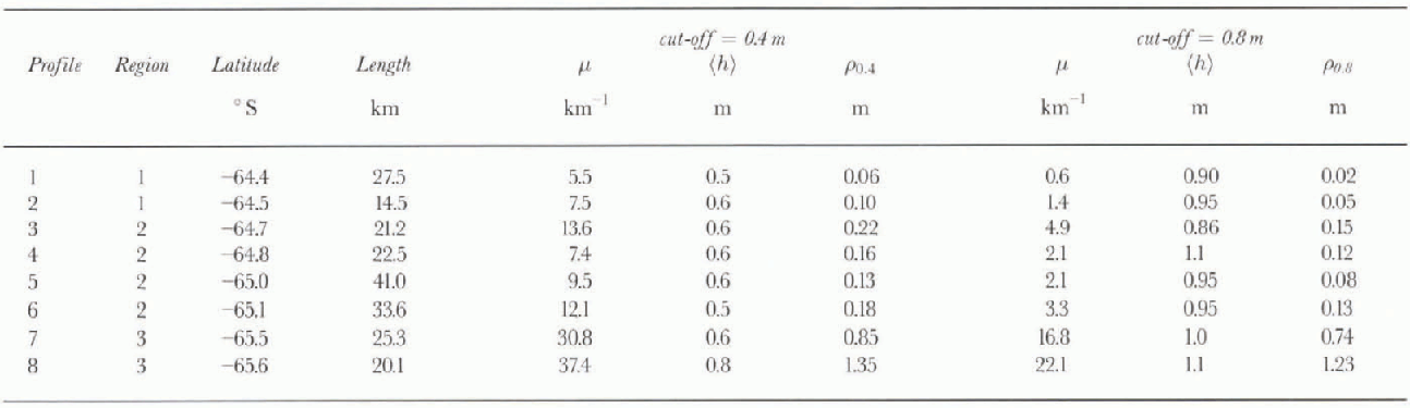
Ridging statistics using minimum ridge cut-off values of 0.4 and 0.8 m

ridges. The area-averaged volume per unit area of ice contained in the ridges, ρ0 can be calculated from:

(4)

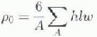
where A is the area over which the volume of all the ridges is summed. Again, we assume that only one-sixth of the total ice volume is contained in the ridge sails. Substituting Equation (3) into Equation (4), and assuming a constant w

(5)

For these data, the sun angle was 13° or less. Consequently, a shadow of 0.5 m, or one pixel, is cast by a ridge or hummock approximately 0.1m high. Using this method, ρ0 can be calculated relatively quickly over large areas. However, it does not provide an independent estimate of h and I. Also, we do not have a measure of X, and a constant value of w for all the photographs will result in an underestimate of ρ0 in regions with higher ridges, and an overestimate of ρ0 in regions of lower ridge heights. Although this method of estimating ρ0 is not as accurate as using Equation (2), it is much less time-consuming.

All hough there are a number of simplifying assumptions in both methods of calculating ρ0, these estimates allow comparison with other studies, and provide the only technique presently available. For both methods, errors in the estimates of ρ0 may occur if there is a large concentration of ridges, or inhere are several high ridges near each other, so that individual shadows are not distinct. Visual inspection of the photographs did not reveal any situations where this happened. At this time of year, the sun is primarily in the north, and any predominant ridge orientation will bias the results. The observed ridges appeared to be randomly oriented, with most ridges less than 30 m long. Long, linear ridge features are seldom observed in the SAR images. Using a factor of 5 for the ratio of the upper to the lower volume of ice, and a constant ß and w, may result in errors of as much as 20% for any single estimate. However, the equivalent ice thickness contained in ridges for different regions is comparable.

Results

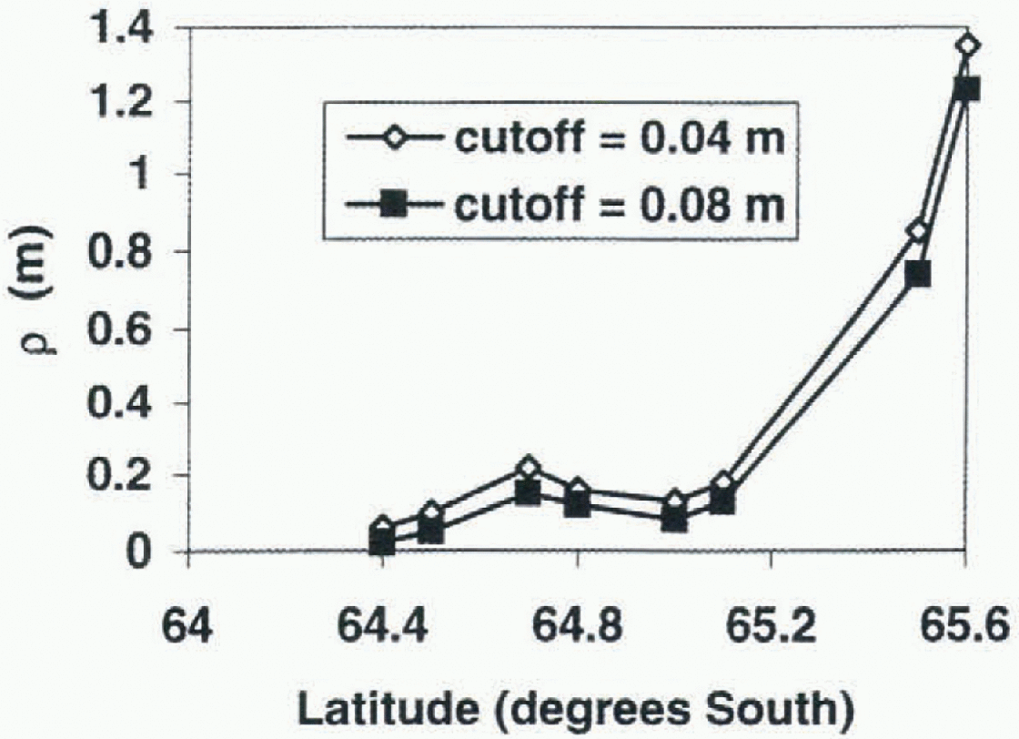
Eight different ridge height distributions were estimated, using 3-5 consecutive photographs. The transect length varied from 14.5 to 41km. The ridge statistics (ρ, μ and computed using minimum ridge heights of 0.4 and 0.8 m, are shown in Table 1, and ρ is plotted in Figure 3. These cut-off heights allow comparison of the results with other studies of ridge heights from laser or acoustic studies (e.g. Lytle and Ackley, 1991; Dierking, 1995). Using a 0.4 m cut-off height, (h) was relatively constant at 0.5 or 0.6 m, with the exception of profile . On the other hand, p varied from 5.5 to 37.4 km⁻¹, with lower values found to the north. Estimates of varied from 0.06 to 1.35 m. Consequently, for an average undeformcd ice thickness of 0.5 m in the region, 11-73% of the ice volume is contained within ridges. The highest p and p values were found around 65.6° S, reflecting the large proportion of highly deformed ice in this region (Fig. 3).

Examples of photographs from different regions of the pack are shown in Figure 4. figure 4a was taken at about 64.4° S. Although the surface of the floes appears rough, high ridges are infrequent. The largest floes are about 200m in diameter, decreasing to the north (Lytle and others, 1998).figure 4b was collected at around 65.0°S, and is an example of the vast floes with minimal surface ridging that were commonly seen in the ice observations. figure 4c, collected at 65.5° S, illustrates the high deformation in this region.

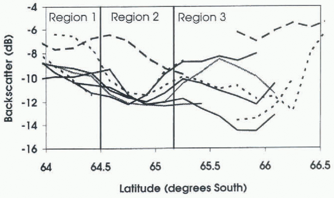
The SAR images contain fealtires similar to those in the more detailed photographs. A region of large floes is centred on 65° S. To the north, there are smaller floes and higher σ ^∘; to the south cr increases and individual floes are generally unresolvable (Fig. 1). The net ice drift was westward al about 17 km d⁻¹. Although the ice floes in llie study region had been replaced during the 3 week experiment, these general features are still seen in all the SAR images. σ ^∘ as a function of latitude for all SAR images is plotted in Figure 5.

Fig. 3.

and calculated using Equation (2).

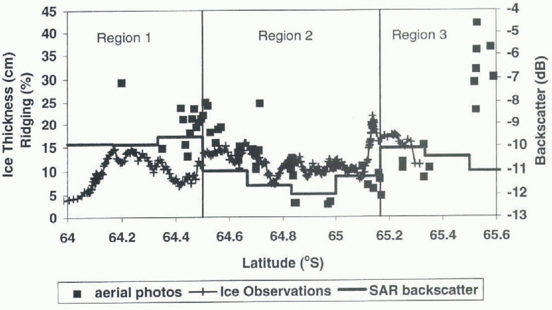
Fifty-nine photographs were analyzed and po was calculated using Equation (5). We have no direct measurements of w, and estimate it using the results from ridge distributions. For ß = 25° and (h) = 0.5 m (the average height found in the ridge distributions for a cut-off of 0.4 m), w= 1.1m. Because this method includes ridges with heights as low as 0.1 m, we arbitrarily reduce น) to 1 m for these calculations. This is probably still a high estimate in regions with lower average ridge height. These results are plotted in Figure 6, where each point represents a single photograph with an area of approximately 1 km². The general trends seen in the ridge distributions are also apparent in Po, with the highest values of Po found towards the south. Variations on scales of 1 km² can be quite large. For example, near 65.5° S, Po varies from 22 to 45 cm within 5 km. The areal extent of ridging estimated from the ship-based ice observations (Fig. 6) is highly variable, ranging from 4% to 22%. It is al a maximum around 65.15° S, and above 10% from this latitude to the southern limit of the observations at 65.4° S.

The data are divided into three different regions, based on σ ^∘ visual inspection of the SAR images and the calculated ridge statistics. These are not distinct or absolute boundaries, but rather general regions with different ridging characteristics.

Region 2 (64.5-65.2°S)

Both the photographs and the ship-based observations indicate that ice in this region is less deformed than the ice to the south. Large (>1km) floes are clearly visible in the SAR image, and are confirmed by the ship-based observations. Using a cut-off height of 0.4 m, p decreases to 7-9 km⁻¹ near 65° S, and ρ0 is reduced to 0.13-0.16 m. in the SAR images, this region has a consistently low σ ^∘ of 12 dB. This does not vary by more than about 0.2 dB during August 1995, indicating that the ice properties which influence the SAR back-scatter did not change significantly on a synoptic scale. The ship-based ice observations confirm this; for the 3 week experiment, they show only a small net increase in the mean thickness of the level ice from 0.46 to 0.54 m, and no lil t change in the areal extent of surface ridging of 10% (Worby and others, 1996a, b). Buoy arrays deployed on the ice in the region moved rapidly; however, they were generally divergent, which is an additional indication of lower ridging. The SAR data from 1996 show one day (10 August 1996) whereσ ^∘ increased to about -7 dB (Fig. 5). On inspection of the image, this region appears to have smaller floes broken up by incoming swell. These SAR data were fail best cast, and may reflect a different sca-icc regime or be an example of the ocean swell penetrating further into the pack than normal.

Fig. 4.

Photographs of sea ice at (a) 64.4° S, (b) 65.0° S and (c) 65.5° S. Each image is a 300 m x.WOm subset of a single photograph.

Fig. 5.

SAR backscatter values for five days from 2 August 1995 to 2 September 1995, shown as solid lines. The average σ ^∘ for 6, 9 and 10 August 1996 is plotted as dotted lines.

Comparison with other ridging results

Allison and Worby 1991 found that regions of low deformation were common directly north of the fast ice. Several of the SAR images show open water regions to the north of the fast ice; the photographs taken in this region also show extensive regions of open water and nilas, with very lew ridges. Increased ridging near the coast, in region 3, is consistent with the results of Dierking (1995; and Lytle and Ackley (1991; in the Wcddell Sea, who used cut-off heights of 0.8 and 0.75m. respectively. in both these studies, μ was highest near the coast, and decreased rapidly away from the highly deformed coastal zone. Our results () are at the. lower end of the range 8-52 km⁻¹ reponed by Dierking (1995) near the coast at 9°W. and higher than the 10.5 km⁻¹ reported by Lytle and Ackley (1991) near 2° E. Weeks and others (1989) used a 0.9 m cut-off for data from the Ross Sea. They found μ decreased from 6.8 km^-1 near the coast to 0.5 km ⁻¹ in the non-coastal regions.

The low μ found north of this coastal deformation zone (0.6-4.9) is slightly lower than the range 3.2-10.4 km ⁻¹ reported by Dierking (1995), and slightly higher than the range 0.6-1.7 km ⁻¹ reported by Lytle and Ackley (1991) for the central Weddell Sea. Our average ridge heights are approximately 0.1 m higher than those reported by Lytle and Ackley (1991) and about 0.1 0.3 m lower than those reported by Dierking (1995).

Fig. 6.

Three different ridging estimates as a function of latitude. The areal extent of ridging (%) as eslimatedfroin ship-based ice observations is shown as plus signs. The equivalent ice thickness, ρ0 in (cm), estimated from individual photographs each approximately 1 km² is plotted as squares, and σ ^∘ (dB) from the SAR data of 2 August 1995 is plotted as a solid line.

Worby and others (1998), using data from eight voyages to the East Antarctic pack, find a mean areal-surface ridging coverage of approximately 11% and a p which is 0.5—1.3 times the mean level ice thickness with in the pack. For the average ice thickness of 50 em, this is an equivalent ice thickness of 0.25-1.15 m, with in the range of our measurements. It should be noted that the 0.5 M height in the study by Worby and others (1998) was not a cut-off height, but an average sail height, hence smaller ridges were included in the observations.

Conclusions

Pressure ridges can contain most of the total ice volume. in region 3, the deformed ice thickness of 1.35 m is over 2.5 times the undeformed ice thickness of about 0.5 m. Much of the ice volume may be contained in relatively low ridges; 0.04-0.12 m of area-averaged ice thickness is contained in ridges that are 0.4-0.8 m high. Compared to the average undeformed ice thickness in this region of 0.5 m, ignoring these smaller ridges can result in a significant underestimation of the total ice volume. Although (h) was constant for a given cut-offheight, μ varied considerably. The 1996 SAR data indicate that the ridging characteristics identified are a persistent feature. Additional studies are needed to confirm this.

Near the edge of the fast ice, open water or newly forming nilas is observed as the ice is pushed away from the coast. Northward is a zone of highly deformed sea ice with similar ridging statistics to the coastal zones in the eastern Weddell Sea. This ice is probably deformed as it interacts with icebergs or changing ocean currents in the region, lb the north of this highly deformed zone, there is a persistent band, approximately 35 60 km wide, of relatively un-deformed sea ice with vast floes. This undeformed ice has a minimum average σ ^∘ of -12 dB. This low σ ^∘ persisted throughout August 1995, despite the passage of two synoptic systems and the associated changes in wind and ice-floe velocities. North of this undeformed band, the amount of ridging, on average, increases and floe sizes decrease as the incoming ocean swells break up the pack. Both the increased ridging and smaller floe sizes increase σ ^∘.