2. Galileo/GPS TDCP velocity determination

2.1 Observation equation

The observation equation for the carrier-phase measurement can be given as:

(1a)\begin{align}\lambda \varphi _r^{G,s} &= \rho _r^{G,s} + c({\delta_r^G - {\delta^{G,s}}} )+ ({b_r^G - {b^{G,s}}} )- I_r^{G,s} + T_r^{G,s} + \lambda {N^{G,s}} + {\varepsilon ^G}\end{align}

(1b)\begin{align}\lambda \varphi _r^{E,s} &= \rho _r^{E,s} + c({\delta_r^E - {\delta^{E,s}}} )+ ({b_r^E - {b^{E,s}}} )- I_r^{E,s} + T_r^{E,s} + \lambda {N^{E,s}} + {\varepsilon ^E}\end{align}

where $\rho $ is the geometrical distance between the receiver $\; r$ and the satellite s, $\; c$ is light speed; G and E represent GPS and Galileo, respectively; ${\delta _r}$ and ${\delta ^s}$ are the receiver clock offset and satellite clock offset; ${b_r}$ and ${b^s}$ are carrier-phase hardware delay bias for the receiver and satellite; I and T are ionospheric delay and tropospheric delay; N is integer ambiguity; $\varepsilon $ includes multipath and receiver noise.

The TDCP measurements are the time difference of successive carrier-phase to the same satellite at a small sampling interval (Kennedy, Reference Kennedy2003; Van Graas and Soloviev, Reference Van Graas and Soloviev2004). Therefore, carrier-phase hardware delay, as well as the constant integer ambiguity, will be eliminated after differencing. The Saastamoinen and Klobuchar models are used to mitigate the effects of tropospheric and ionospheric delay rates (Zhang et al., Reference Zhang, Zhang, Grenfell and Deakin2008; Freda et al., Reference Freda, Angrisano, Gaglione and Troisi2015). Carrier-phase derived Doppler can be given as:

(2a)\begin{align}\lambda \dot{\varphi }_r^{G,s} &= \dot{\rho }_r^{G,s} + c({\dot{\delta }_r^G - {{\dot{\delta }}^{G,s}}} )+ {\dot{\varepsilon }^G}\end{align}

(2b)\begin{align}\lambda \dot{\varphi }_r^{E,s} &= \dot{\rho }_r^{E,s} + c({\dot{\delta }_r^E - {{\dot{\delta }}^{E,s}}} )+ {\dot{\varepsilon }^E}\end{align}

where dot represents differencing operation. Introducing the receiver position vector ${\boldsymbol{r}_r}$ and satellite position vector ${\boldsymbol{r}^s}$, $\rho $ can be given:

(3a)\begin{align}\rho (t )&= \boldsymbol{e}_r^s(t )\cdot [{{\boldsymbol{r}^s}(t )- {\boldsymbol{r}_r}(t )} ]\end{align}

(3b)\begin{align}\rho ({t - 1} )&= \boldsymbol{e}_r^s({t - 1} )\cdot [{{\boldsymbol{r}^s}({t - 1} )- {\boldsymbol{r}_r}({t - 1} )} ]\end{align}

where $\boldsymbol{e}_r^s$ is the line-of-sight (LOS) unit vector from the receiver r to the satellite $\; s$; t denotes observed epoch. Then geometrical distance variation can be computed by:

(4)\begin{equation}\dot{\rho } = \rho (t )- \rho ({t - 1} )= \boldsymbol{e}_r^s(t )\cdot [{{\boldsymbol{r}^s}(t )- {\boldsymbol{r}_r}(t )} ]- \boldsymbol{e}_r^s({t - 1} )\cdot [{{\boldsymbol{r}^s}({t - 1} )- {\boldsymbol{r}_r}({t - 1} )} ]\end{equation}

Substituting ${\dot{\boldsymbol{r}}_r} = {\boldsymbol{r}_r}(t )- {\boldsymbol{r}_r}({t - 1} )$ and ${\dot{\boldsymbol{r}}^s} = {\boldsymbol{r}^s}(t )- {\boldsymbol{r}^s}({t - 1} )$ in Equation (4), yields:

(5)\begin{equation}\dot{\rho } = \boldsymbol{e}_r^s(t )\cdot [{{{\dot{\boldsymbol{r}}}^s} - {{\dot{\boldsymbol{r}}}_r}} ]- [{\boldsymbol{e}_r^s(t )- \boldsymbol{e}_r^s({t - 1} )} ]\cdot [{{\boldsymbol{r}^s}({t - 1} )- {\boldsymbol{r}_r}({t - 1} )} ]\end{equation}

Hence, the actual velocity is not really instantaneous but averaged in a small interval. Also, it is necessary to store the previous position of satellites and the receiver, which hampers the processing efficiency and real-time implementation. In order to address these issues, first-order central difference approximation was introduced (Cannon et al., Reference Cannon, Lachapelle, Szarmes, Hebert, Keith, Jokerst and Base1997), which can be expressed:

(6)\begin{equation}\dot{\rho } = \boldsymbol{e}_r^s({t - 0.5} )\cdot [{{{\dot{\boldsymbol{r}}}^s}({t - 0.5} )- {{\dot{\boldsymbol{r}}}_r}({t - 0.5} )} ]\end{equation}

where ${\dot{\boldsymbol{r}}^s}({t - 0.5} )$ denotes the instantaneous satellite velocity. Substituting Equation (6) in Equation (2), and omitting epoch notation:

(7a)\begin{align}\lambda \dot{\varphi }_r^{G,s} &= \boldsymbol{e}_r^{G,s} \cdot ({{{\dot{\boldsymbol{r}}}^{G,s}} - {{\dot{\boldsymbol{r}}}_r}} )+ c({\dot{\delta }_r^G - {{\dot{\delta }}^{G,s}}} )+ {\dot{\varepsilon }^G}\end{align}

(7b)\begin{align}\lambda \dot{\varphi }_r^{E,s} &= \boldsymbol{e}_r^{E,s} \cdot ({{{\dot{\boldsymbol{r}}}^{E,s}} - {{\dot{\boldsymbol{r}}}_r}} )+ c({\dot{\delta }_r^E - {{\dot{\delta }}^{E,s}}} )+ {\dot{\varepsilon }^E}\end{align}

Defining GPS as the reference system, the Galileo ISB variation can be written as:

(8)\begin{equation}\dot{\delta }_r^E = \dot{\delta }_r^G + I\dot{S}B\end{equation}

As the satellite velocity and satellite clock drift can be computed by broadcast ephemeris, Equation (7) can be further expressed as:

(9a)\begin{align}\lambda \tilde {\dot{\varphi }}_r^{G,s} &={-} \boldsymbol{e}_r^{G,s} \cdot {\dot{\boldsymbol{r}}_r} + c\dot{\delta }_r^G + {\dot{\varepsilon }^G}\end{align}

(9b)\begin{align}\lambda \tilde {\dot{\varphi }}_r^{E,s} &={-} \boldsymbol{e}_r^{E,s} \cdot {\dot{\boldsymbol{r}}_r} + c\dot{\delta }_r^G + I\dot{S}B + {\dot{\varepsilon }^E}\end{align}

where:

(10a)\begin{align}\lambda \tilde {\dot{\varphi }}_r^{G,s} &= \lambda \dot{\varphi }_r^{G,s} - \boldsymbol{e}_r^{G,s} \cdot {\dot{\boldsymbol{r}}^{G,s}} + c{\dot{\delta }^{G,s}}\end{align}

(10b)\begin{align}\lambda \tilde {\dot{\varphi }}_r^{E,s} &= \lambda \dot{\varphi }_r^{E,s} - \boldsymbol{e}_r^{E,s} \cdot {\dot{\boldsymbol{r}}^{E,s}} + c{\dot{\delta }^{E,s}}\end{align}

Hence, there will be five unknown parameters in the Galileo/GPS combined TDCP method: three velocity components, the receiver clock drift and Galileo ISB variation.

2.2 Stochastic equation

Different observations have different precision, so it is necessary to weight the observations and establish a reasonable stochastic model. When positioning, the user equivalent range error is generally used to determine the weight. Similarly, errors of carrier-phase derived Doppler can be divided into two parts, namely: space-related error and signal-propagation-related error. The space-related error comprises the satellite orbit and clock errors, whereas signal-propagation-related error includes atmospheric transmitting delay, multipath and receiver noise. Therefore, the standard deviation of the observation can be expressed as:

(11)\begin{equation}{\sigma ^2} = \sigma _{orb}^2 + {\sigma ^2}({Ele} )\end{equation}

where $\sigma $ denotes the standard deviation of the observation; $\; {\sigma _{orb}}$ denotes the standard deviation of the satellite velocity and clock drift; $\; \sigma ({Ele} )$ denotes the standard deviation of signal propagation errors, including tropospheric and ionospheric delay rate, multipath and receiver noise.

The orbit error, including the error of satellite position, velocity and clock drift in velocity determination, has been analysed in detail for GPS (Zhang et al., Reference Zhang, Zhang, Grenfell and Deakin2008). However, there are only a few studies on these effects for Galileo. Considering the signal-in-space range error of 30 cm for Galileo broadcast ephemeris and clock (Steigenberger and Montenbruck, Reference Steigenberger and Montenbruck2016) and the small order of clock drift (Zheng and Tang, Reference Zheng and Tang2015), this study will focus on the accuracy of satellite velocity for all 24 satellites. Generally, there are two methods to calculate the satellite velocity: position differential and closed-form formula. Some literature shows that the accuracy of the two methods is the same, but the position differential method is simple to implement (Zhang et al., Reference Zhang, Zhang, Grenfell and Deakin2006; Zheng and Tang, Reference Zheng and Tang2015). With this consideration, the position differential method is adopted here to calculate Galileo satellite velocity:

(12)\begin{equation}{\dot{\boldsymbol{r}}^s} = \frac{{{\boldsymbol{r}^s}({t + \Delta t} )- {\boldsymbol{r}^s}({t - \Delta t} )}}{{2\Delta t}}\end{equation}

where $\Delta t$ denotes a small interval. Taking velocity from the precise ephemeris linear interpolation as the true value, the broadcast velocity precision is well within 0⋅5 mm/s except two elliptical orbit satellites (E14 and E18), as shown in Figure 1. Here, $\Delta t$ is made to equal 0⋅001 s and the broadcast ephemeris of day of year (DOY) 152 in 2019 is adopted. The accuracy in radial, along and cross components is nearly the same, whereas Galileo and GPS are comparable. Additionally, it is obvious that the accuracy of E14 and E18 are beyond 2 mm/s, which will certainly destroy the determination of velocity. Further research finds that the signal health status of E14 and E18 is set to ‘Test’, which means that these two satellites are currently being tested (Paziewski et al., Reference Paziewski, Sieradzki and Wielgosz2018; Robustelli et al., Reference Robustelli, Benassai and Pugliano2019). Therefore, E14 and E18 are not included to process in this paper.

Figure 1.

RMS of satellite velocity from the broadcast ephemeris (2019/06/01, DOY 152): (a) Galileo and (b) GPS

Signal propagation error, including ionospheric delay, tropospheric delay and multipath, is elevation-dependent. However, most studies have focused on the field of positioning. This study adopts dual frequency observations to investigate the relationship between elevation angle and carrier-phase derived Doppler. Considering Equation (2), the carrier-phase derived Doppler of ${L_1}$ (E1) and ${L_2}$ (E5a) can be written as:

(13a)\begin{align}\lambda {\dot{\varphi }_1} &= \dot{\rho } + c({{{\dot{\delta }}_r} - {{\dot{\delta }}^s}} )+ {\dot{\varepsilon }_1}\end{align}

(13b)\begin{align}\lambda {\dot{\varphi }_2} &= \dot{\rho } + c({{{\dot{\delta }}_r} - {{\dot{\delta }}^s}} )+ {\dot{\varepsilon }_2}\end{align}

Then we can eliminate receiver-dependent terms after differencing:

(14)\begin{equation}\lambda \Delta {\dot{\varphi }_{12}} = \lambda {\dot{\varphi }_1} - \lambda {\dot{\varphi }_2}\end{equation}

where $\Delta {\dot{\varphi }_{12}}$ can reflect the noise of carrier-phase derived Doppler. Figure 2 shows the variations of $\Delta {\dot{\varphi }_{12}}$ in mm/s with respect to time. The data are from the multi-GNSS experiment (MGEX) station KITG and two satellites with longer observation arcs are selected. As can be seen from Figure 2, the observation noise and elevation angle are dependent. The larger noise at the edges is due to the low-elevation rays at the rising and setting of the satellite. Based on this result, an ESM can be proposed:

(15)\begin{equation}{\sigma ^2}({Ele} )= {\raise0.7ex\hbox{${\sigma _0^2}$} \!\mathord{/ {\vphantom {{\sigma_0^2} {2sin({Ele} )}}} }\!\lower0.7ex\hbox{${2sin({Ele} )}$}}\end{equation}

where ${\sigma _0}$ can be 2⋅8 mm/s in 1 s sample, which take accuracy of carrier-phase as 2 mm. Here, the same ${\sigma _0}$ for GPS and Galileo can be adopted based on the analysis of Galileo/GPS signals (Tian et al., Reference Tian, Sui, Xiao, Zhao and Tian2019).

Figure 2.

The noise and elevation angle of carrier-phase-derived Doppler with respect to time for (a) E12 and (b) E24 (KITG station, 2019/04/10, 08:00:00~16:00:00)

3. Simplified and unified Galileo/GPS TDCP method

All the parameters in Equation (9) can be solved by performing the least-square estimation with normal equation. Based on the normal equation, correlation coefficients and scaled sensitivity matrix can be used to analyse the relationship between ISB variation and other parameters. Correlation coefficients can be acquired by the following function:

(16)\begin{equation}r = \frac{{\sigma ({I\dot{S}B,x} )}}{{{\sigma _{I\dot{S}B}}{\sigma _x}}}\end{equation}

where $\sigma ({I\dot{S}B,x} )$ denotes co-variance between $I\dot{S}B$ and other parameters x (velocity in East, North and Up and receiver clock drift). Still using data from station KITG, we compute ISB variation and correlation coefficients, as shown in Figure 3. It can be observed that the mean value of ISB variations is nearly zero and correlation coefficients with clock drift and Up component are obvious, whereas correlation coefficients with East and North components are nearly negligible. In other words, ISB variations, not considered, will mainly be assimilated by clock drift and Up component. Additionally, the sum of correlation coefficients with Up component is nearly zero, whereas correlation coefficients with clock drift are always negative. Therefore, ISB variations will slightly affect the Up component in the whole time period.

Figure 3.

ISB variation and its correlation coefficients with East, North and Up components and receiver clock drift (KITG station, 2019/04/10, 08:00:00~16:00:00)

To assess quantitatively the influence of ISB variation on other parameters, namely three velocity components and the receiver clock drift, the scaled sensitivity matrix method is used (Dong et al., Reference Dong, Fang, Bock, Cheng and Miyazaki2002; Chen et al., Reference Chen, Zhang, Wang, Yang, Dong, Wang, Qu and Wu2015). Equation (9) can be written in the following form:

(17)\begin{equation}\boldsymbol{y} = \boldsymbol{A} \cdot \boldsymbol{x} + \boldsymbol{B} \cdot I\dot{S}B\end{equation}

where $\boldsymbol{y}$ is observation matrix; $\boldsymbol{A}$ and $\boldsymbol{B}$ are the design matrix; and$\; \boldsymbol{x}$ is other unknown parameters matrix. The corresponding solution is:

(18)\begin{equation}\begin{aligned} \hat{\boldsymbol{x}} & ={({{\boldsymbol{A}^{\boldsymbol{T}}}\boldsymbol{PA}} )^{ - 1}}{\boldsymbol{A}^{\boldsymbol{T}}}\boldsymbol{P}({\boldsymbol{A} \cdot \boldsymbol{x} + \boldsymbol{B} \cdot I\dot{S}B} )\\ & =\bar{\boldsymbol{x}} + {({{\boldsymbol{A}^{\boldsymbol{T}}}\boldsymbol{PA}} )^{ - 1}}{\boldsymbol{A}^{\boldsymbol{T}}}\boldsymbol{PB} \cdot I\dot{S}B \end{aligned}\end{equation}

where $\boldsymbol{P}$ is the weight matrix; $\; \bar{\boldsymbol{x}}$ is the solution without $I\dot{S}B$; $\boldsymbol{S} = {({{\boldsymbol{A}^{\boldsymbol{T}}}\boldsymbol{PA}} )^{ - 1}}{\boldsymbol{A}^{\boldsymbol{T}}}\boldsymbol{PB}$ is the scaled sensitivity matrix. The scaled sensitivity matrix is calculated using the normal equation of KITG station and mean values are shown in Table 1, where less than 10% of ISB variations are assimilated by three velocity parameters and the main parts of ISB variations are assimilated into clock drift. Another issue is that the sum of elements is not equal to one, which means that some of the ISB variations go into residuals.

Table 1.

Elements of the scaled sensitivity matrix between ISB variation and other parameters

The difference values in three velocity components can then be obtained by multiplying ISB variation and the element of the scaled sensitivity matrix, as shown in Figure 4. It is obvious that the difference distribution is a Gaussian normal distribution and most differences are less than 0⋅5 mm/s. Mean values are nearly zero and standard deviations are less than 0⋅4 mm/s in three velocity components, which shows that ISB variations can be removed from the observation equation. After removing ISB variation, the observation equation can be written as:

(19a)\begin{align}\lambda \tilde {\dot{\varphi }}_r^{G,s} &={-} \boldsymbol{e}_r^{G,s} \cdot {\dot{\boldsymbol{r}}_r} + c\dot{\delta }_r^G + {\dot{\varepsilon }^G}\end{align}

(19b)\begin{align}\lambda \tilde {\dot{\varphi }}_r^{E,s} &={-} \boldsymbol{e}_r^{E,s} \cdot {\dot{\boldsymbol{r}}_r} + c\dot{\delta }_r^G + {\dot{\varepsilon }^E}\end{align}

Figure 4.

Epoch difference distribution in East, North and Up components (KITG station, 2019/04/10, 08:00:00~16:00:00)

In this new model, observations from Galileo and GPS can be processed in a unified way as they are the same system. It is beneficial to solve the problem of insufficient number of satellites in a challenging environment.

4. Static test

In order to validate the performance of the proposed stochastic model and unified Galileo/GPS function model in TDCP velocity determination, five scenarios were designed, namely: scenario 1, only Galileo with EWR; scenario 2, only Galileo with ESM; scenario 3, Galileo/GPS with EWR; scenario 4, Galileo/GPS with ESM; scenario 5, unified Galileo/GPS with ESM. The ISB variations are considered in scenario 4, but not in scenario 5.

Because true velocity is zero, 1 Hz sample data from 10 MGEX static stations during 08:00~16:00 on DOY 100 of 2019 is used first. Figure 5 shows the distribution of 10 stations, which can simultaneously observe Galileo and GPS. In actual data processing, only L1(E1) data are used for single point positioning and velocity determination, with epoch by epoch and a cut-off angle of 10°.

Figure 5.

Distribution of 10 MGEX stations used for velocity determination assessment

Figure 6 illustrates the satellite sky plot of Galileo and GPS in the KITG station during the time period for data collection. The centre of the sky plot is the receiver position and the distance to the centre is a multiple of unit distance and cosine of elevation angle. It can be seen that there are more than five satellites for the individual satellite system, which can be enough to estimate receiver velocity.

Figure 6.

Satellite sky plot of Galileo (left) and GPS (right) (KITG station, 2019/04/10, 08:00:00~16:00:00). Different colors represent different satellites

The RMS of each station is shown in Figure 7 and the mean value of root mean square (RMS) is shown in Table 2. It can be seen that with Galileo/GPS combined, TDCP velocity achieves the better performance compared with Galileo-only TDCP velocity. And, on the whole, TDCP velocity with ESM can improve velocity accuracy when compared with the EWR model, especially in East and Up components. The accuracy of Galileo/GPS with ISB variation (GGS + ESM) is nearly the same as that of Galileo/GPS with the unified Galileo/GPS model (Unified GGS + ESM). Regarding determination of Galileo-only TDCP velocity, DAEJ has the worst velocity performance in the Up component, which may be due to fewer satellites and more cycle slips after investigating the observation file.

Figure 7.

RMS of velocity differences for each station in the East, North and Up components, where GAL represents Galileo-only solution (left) and GGS represents Galileo/GPS combined solution (right)

Table 2.

Mean RMS of velocity differences for all stations

^a GGS represents scenario 5.

Overall, comparing the RMS values in Table 2, it can be seen that the Galileo/GPS combined velocity solution can bring improvements of about 1 mm/s, 0⋅5 mm/s, 2⋅5 mm/s in the East, North and Up components, respectively. ESM can improve the accuracy of velocity determination, especially in East and Up components, in comparison with EWR. And the ESM-induced improvements in Galileo/GPS solution are more significant than in the Galileo-only solution, which is because the combined system has more visible satellites. Additionally, the accuracy of the unified Galileo/GPS velocity solution can be nearly consistent with that of the traditional solution in the East, North and Up components.

5. A real vehicle test

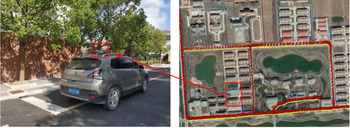
The kinematic test was conducted by a car and dual carrier-phase and code measurements were collected with 1 Hz logging rate by iRTK5 GNSS receiver (see Figure 8, left). The iRTK5 GNSS receiver supports full constellation and multiple channels with Maxwell7 technology, which can achieve a four-constellation and triple-frequency solution. Meanwhile another iRTK5 receiver was installed in an open area as a reference station.

Figure 8.

The vehicle used to perform the mission (left) and the main trajectory of the test (right). The red rectangle in the right picture represents the position of the GNSS receiver (left)

Most of the test session had a good LOS view of the whole sky, whereas some satellites at a few epochs were blocked by some buildings and trees near the road. The main trajectory of the vehicle test is shown in Figure 8 (right). In order to fully evaluate the performance of velocity determination, four overlapped loops were implemented in the same path. The test was conducted on 3 August 2019. The duration of the vehicle test was about 45 min, from 09:12 to 09:57, GPS time.

The number of satellites tracked during the test is shown in Figure 9 (left) and the corresponding position dilution of precision (PDOP) is shown in Figure 9 (right). It can be seen that the number of satellites in the Galileo-only case is about four or five and in the GPS-only case about five or six, whereas the Galileo/GPS (GGS) combined case could reach about 10 or more in most epochs. Accordingly, compared with Galileo-only or GPS-only, PDOP turns out to be much lower when using the Galileo/GPS combined system. As for Galileo, the PDOP is worse than GPS because there is not complete coverage from the Galileo satellites in orbit.

Figure 9.

Number of satellites tracked in the test (left) and PDOP of every epoch in the test (right)

It is rather difficult to evaluate the kinematic velocity results, because a ‘reference solution’ is not easy to establish. In this case, we use the reference velocity solution derived through numerical differentiation of the receiver positions that are processed by fixing double-difference ambiguities (Ding and Wang, Reference Ding and Wang2011; Zheng and Tang, Reference Zheng and Tang2015). Commercial software, named inertial explorer (IE) with version 8⋅80, was used and velocity solutions with Galileo/GPS dual carrier-phase measurements in three components are shown in Figure 10.

Figure 10.

Velocity solutions in East, North and Up components from DGPS with first-order central difference of a Taylor series approximation

In kinematic processing, five schemes are used, the same as in the static test. Every epoch is solved by least squares method, with a cut-off angle of 10°. As with the static test, only L1(E1) data are used. Figure 11 shows velocity differences for scenarios 1–4, where horizontal outliers with greater than 2 cm/s and vertical outliers with greater than 5 cm/s are excluded.

Figure 11.

Velocity differences with the reference velocity in East, North and Up components for four scenarios

It can be seen that, compared with the Galileo-only velocity solution, the Galileo/GPS combined velocity solution has lower noise levels in the East, North and Up components, respectively. Compared with the Galileo/GPS velocity solution with EWR, the Galileo/GPS velocity solution with ESM can improve the accuracy of velocity determination, especially in the North component. In addition, the number of Galileo-only valid epochs is less than that of the Galileo/GPS combined system, which is mainly because there are not enough valid solutions in some poor observation environments.

Table 3 presents a summary of velocity differences in the East, North and Up components and valid epochs for five scenarios. It can be seen that, compared with the Galileo-only velocity solution, the Galileo/GPS combined velocity solution can bring improvements of about 2⋅0 mm/s, 0⋅5 mm/s, 1⋅5 mm/s in the East, North and Up components, respectively and valid epochs can be improved by 15%. ESM-induced improvements in the Galileo/GPS solution are 0⋅4 mm/s, 0⋅6 mm/s in North and Up components, whereas those in the Galileo-only solution are 0⋅01 mm/s and 0⋅13 mm/s. This is mainly because there are only four or five Galileo satellites that can be used and their elevation angles are mostly more than 30° in the Galileo-only solution.

Table 3.

RMS of velocity differences of five scenarios and valid epochs in kinematic test

^a GGS represents scenario 5.

Additionally, the velocity differences are less than 0⋅1 mm/s,0⋅1 mm/s and 0⋅2 mm/s in the East, North and Up components when compared with the traditional Galileo/GPS velocity solution and unified Galileo/GPS velocity solution. It can also be seen that the valid epochs of the unified Galileo/GPS velocity solution are nearly consistent with those of the traditional Galileo/GPS velocity solution.

In order to show the superiority of unified Galileo/GPS, some satellites were excluded to simulate the condition of fewer visible satellites. In the simulated challenging case, E07, E08, E13, G02, G05 and G13 are selected, as they have higher elevation angles. But there are many cycle slips for G02 and G05 at 09:33–09:42, in which the traditional Galileo/GPS solution cannot be obtained. Figure 12 depicts velocity differences for traditional and unified velocity solution, where horizontal outliers with greater than 5 cm/s and vertical outliers with greater than 10 cm/s are excluded.

Figure 12.

Velocity differences in East, North and Up components in the challenging case

In Figure 12, it can be seen that, due to the severe cycle slips, the number of available satellites is less than five, which makes the traditional Galileo/GPS velocity unsolvable. However, when using the unified Galileo/GPS model a high accuracy of velocity solution can still be obtained, which shows the superiority of the unified model.