1 Introduction
Aerofoil–turbulence interaction (ATI) is one of the fundamental noise generation mechanisms in the field of aeroacoustics. It is predominantly generated by surface pressure fluctuations close to the aerofoil leading edge (LE) and arises due to the rapid distortion of the vorticity field impinging on it (Amiet Reference Amiet1975; Goldstein Reference Goldstein1978). ATI noise is an important mechanism in a number of applications including wind turbines, aero-engines, propellers, fans, high-lift devices, etc. The classical theory by Amiet (Reference Amiet1975) provides a first-order prediction of ATI by considering turbulence convecting in a uniform mean flow that suddenly undergo a no-flow boundary condition normal to a flat plate. The theory predicts that a fluctuating pressure dipole source is induced on the surface which then radiates to the far field. Howe’s theory (1989 and 2003) on vortex sound explains the ATI noise in a similar fashion by considering that the velocity field generated by a vortex close to an aerofoil induces dipole sources on the aerofoil surface proportional to the fluctuating normal forces. Both the Amiet and Howe solutions give consistent predictions of the far-field noise in the low Mach number limit.
ATI noise can be the dominant source when the level of turbulence intensity impinging on the aerofoil is sufficiently high (Migliore & Oerlemans Reference Migliore and Oerlemans2004), which is often the case, for example, at the LE of outlet guide vanes (OGV) in a turbofan engine. The effects of variations in aerofoil geometry such as angle of attack, aerofoil thickness, camber, etc, on ATI noise have been studied by Atassi, Subramaniam & Scott (Reference Atassi, Subramaniam and Scott1990), Lockard & Morris (Reference Lockard and Morris1998), Evers & Peake (Reference Evers and Peake2002), Devenport, Staubs & Glegg (Reference Devenport, Staubs and Glegg2010), Roger & Carazo (Reference Roger and Carazo2010), Roger & Moreau (Reference Roger and Moreau2010), Ayton & Peake (Reference Ayton and Peake2013), Gill, Zhang & Joseph (Reference Gill, Zhang and Joseph2013) and Kim, Lee & Cheong (Reference Kim, Lee and Cheong2015). Most of this work has been based on two-dimensional turbulence or harmonic vortical gusts at low free-stream Mach numbers.
Undulated LEs (with tubercles, protuberance or waviness) inspired by the flippers of humpback whales (Fish & Battle Reference Fish and Battle1995; Miklosovic et al. Reference Miklosovic, Murray, Howle and Fish2004) have been studied in recent years with regard to their benefits in terms of improved aerodynamic/hydrodynamic performance, particularly at high angles of attack close to the stall (Johari et al. Reference Johari, Henoch, Custodio and Levshin2007; Hansen, Kelso & Dally Reference Hansen, Kelso and Dally2011; Yoon et al. Reference Yoon, Hung, Jung and Kim2011; Guerreiro & Sousa Reference Guerreiro and Sousa2012; Zhang, Wang & Xu Reference Zhang, Wang and Xu2013; Skillen et al. Reference Skillen, Revell, Pinelli, Piomelli and Favier2014). Most of this work demonstrates that these LE modifications significantly improve the post-stall characteristics whereas they may adversely affect the pre-stall performance. The adverse effect, however, can be reduced by optimising the profile of the LE undulation (Hansen et al. Reference Hansen, Kelso and Dally2011). Again, most of the work was based on incompressible or low-Mach-number flows.
In comparison to the aerodynamic aspects, the understanding of aeroacoustic effects of the undulated LEs has been underdeveloped. Hansen, Kelso & Doolan (Reference Hansen, Kelso and Doolan2012) observed experimentally a reduction in aerofoil tonal noise by applying undulated (sinusoidal) LEs to a NACA0021 aerofoil at a Reynolds number of
 $1.2\times 10^{5}$
. The formation of streamwise vortices behind the roots of the sinusoidal LE profile were identified as being the reason for the reduction in tonal self-noise by breaking up the coherence of vortex generation at the trailing edge. Similar observations have also been made by Arndt & Nagel (Reference Arndt and Nagel1972), Hersh, Soderman & Hayden (Reference Hersh, Soderman and Hayden1974) and Longhouse (Reference Longhouse1977) using sawtooth-type LE serrations.
The main focus of this paper is on the reduction of ATI noise achieved by using sinusoidal wavy LEs. Preliminary investigations on their effectiveness have recently been reported. Lau, Haeri & Kim (Reference Lau, Haeri and Kim2013) performed 3-D nonlinear Euler simulations of the noise radiation due to a flat plate and a symmetric NACA (from 0050 to 0020) aerofoil with various wavy LE (WLE) profiles situated in a mean flow (
 $M_{\infty }=0.4$
–0.6) with a harmonic vortical gust. The radiated noise levels were consistently lower than those from the straight LE (SLE) cases. However, this study used single- and double-frequency vortical gust functions rather than realistic turbulent flows. They observed that the level of gust-response noise decreased significantly with increasing amplitude of the WLE profile (
 $h_{LE}$
) whereas the wavelength of WLE (
 ${\it\lambda}_{LE}$
) had an insignificant impact. The ratio of the WLE amplitude to the streamwise wavelength of the incident gust (
 $h_{LE}/{\it\lambda}_{g}$
) was shown to be a major similarity parameter in determining the level and the directional profile of the noise reduction. They also observed the noise-reduction effects of WLE for various aerofoil thicknesses and flow incidence angles. Clair et al. (Reference Clair, Polacsek, Garrec, Reboul, Gruber and Joseph2013) confirmed the noise-reduction effect of WLE based on a
 $\text{NACA65}_{1}$
-210 aerofoil (in low-speed flows) both numerically and experimentally although the numerical predictions deviated significantly from the measured noise spectrum. This was attributed to the fact that velocity fluctuations in the simulations were confined to the vertical direction only.
Based on the recent observations discussed above, the authors aim to identify and understand the mechanisms by which WLEs can reduce ATI noise. In this study, high-order accurate numerical simulations of the ATI event are performed for a flat-plate aerofoil situated in an inviscid mean flow containing homogeneous isotropic turbulence generated upstream. This study neglects various other factors that are likely to influence noise radiation such as aerofoil thickness/camber, flow incidence angle, turbulence anisotropy, viscosity, etc. The current numerical simulations provide time histories of pressure and velocity fluctuations on both the aerofoil surface and the far field, which allows spectral and correlation analyses to be performed to help identify the dominant noise sources. We note that these quantities are hard to obtain experimentally owing to the difficulty with determining the surface pressure fluctuations near the LE. Two main mechanisms underlying noise reductions with WLE are shown to be source cutoff and phase interference effects existing in the surface pressure fluctuations along the LE.
This paper is organised as follows. First the problem under investigation is carefully defined and the computational set-up for high-order accurate simulations are described in § 2. Some initial observations and investigations of the simulation results relating to overall mean square pressure and correlations are provided in § 3. Spectral analysis of the predicted time history of the pressure fluctuations is presented in § 4 where the source cutoff and phase interference effects along the LE are discussed as dominant noise-reduction mechanisms associated with WLE. Finally, concluding remarks are given in § 5.
2 Current ATI problem and the computational set-up
The essential elements of the aerofoil–turbulence interaction (ATI) problem are illustrated in figure 1. The computational domain in a rectangular cuboid contains a flat-plate aerofoil at the centre with zero thickness and zero angle of attack. The longitudinal and vertical boundaries of the domain are surrounded by a sponge layer through which the flow is (gently) forced to maintain the potential mean flow condition. Any acoustic waves are attenuated and absorbed in the sponge layer to prevent numerical reflections at the outer boundaries. The lateral boundaries of the domain are interconnected via a periodic boundary condition. The aerofoil has a WLE (wavy LE) which is profiled by using a sine function where the most protruded points are defined as ‘peak’, the least as ‘root’ and the middle as ‘hill’ as denoted in figure 2. In the current simulations, the spanwise length of the domain is set to cover two wavelengths of the WLE profile given. As shown in figure 1, ATI noise is simulated by injecting synthetically generated turbulence into the uniform mean flow through the upstream boundary via the sponge layer. The synthetic turbulence, free of artefact noise, is constructed by using randomly distributed divergence-free vortical eddies leading to homogeneous isotropic turbulence based on von Kármán velocity spectra (details to follow).
Illustration of the present computational set-up for the simulation of ATI noise. A snapshot of
 $v$
-velocity field normalised by the ambient speed of sound. The mean flow is in the horizontal direction from left to right.

Surface meshes on the flat-plate aerofoils used in the present study of ATI noise; (a) with a straight leading edge (SLE); and (b) with a wavy leading edge (WLE). The case of
 $h_{LE}/L_{c}=1/15$
and
 ${\it\lambda}_{LE}/L_{c}=2/15$
is shown in this figure.

The free-stream Mach number is set to
 $M_{\infty }=u_{\infty }/a_{\infty }=0.24$
. This Mach number corresponds to the flow speed (
 $u_{\infty }=80~\text{m}~\text{s}^{-1}$
) used in a previous wind-tunnel experiment by Narayanan et al. (Reference Narayanan, Chaitanya, Haeri, Joseph, Kim and Polacsek2015). Herein,
 $L_{c}$
denotes the mean chord length of the aerofoil,
 $L_{z}$
is the span of the aerofoil,
 $h_{LE}$
is the amplitude of WLE (
 $2h_{LE}$
being the peak-to-root amplitude) and
 ${\it\lambda}_{LE}$
is the spanwise wavelength of WLE. The WLE profile in this study is defined by
 $$\begin{eqnarray}x_{LE}=-\frac{1}{2}L_{c}+h_{LE}\sin \left(\frac{2{\rm\pi}z}{{\it\lambda}_{LE}}\right),\quad z\in \left[-\frac{1}{2}L_{z},\frac{1}{2}L_{z}\right],\end{eqnarray}$$
where the location of the trailing edge is fixed at
 $x_{TE}=(1/2)L_{c}$
. The wavelength of the WLE in the current study is set to
 ${\it\lambda}_{LE}/L_{c}=2/15$
and the baseline amplitude of WLE is
 $h_{LE}/L_{c}=1/15$
. The value of
 $h_{LE}$
may vary in some cases where the effect of
 $h_{LE}$
is discussed. The span of the aerofoil (domain length in the
 $z$
-direction) is set to
 $L_{z}=2{\it\lambda}_{LE}$
as mentioned earlier. These geometric parameters are chosen as they were used in the previous wind-tunnel experiment (Narayanan et al.
Reference Narayanan, Chaitanya, Haeri, Joseph, Kim and Polacsek2015). The current computational set-up was validated against the previous experiment as reported in Kim & Haeri (Reference Kim and Haeri2015).
2.1 Governing equations and numerical methods
This section introduces the governing equations and computational methods used in the present simulation of ATI noise. The governing equations employed are full 3-D compressible Euler equations (with a source term for the sponge layer mentioned earlier) in a conservative form transformed into a generalised coordinate system:
 $$\begin{eqnarray}\frac{\partial }{\partial t}\left(\frac{Q_{i}}{J}\right)+\frac{\partial }{\partial {\it\xi}_{j}}\left(\frac{\boldsymbol{F}_{i}\boldsymbol{\cdot }\boldsymbol{e}_{k}}{J}\frac{\partial {\it\xi}_{j}}{\partial x_{k}}\right)=-\frac{a_{\infty }}{L_{c}}\frac{S_{i}}{J},\end{eqnarray}$$
where
 $i=1,\ldots ,5$
;
 $j=1,2,3$
; and
 $k=1,2,3$
. In (2.2), the conservative variables and the flux vectors are given by
 $$\begin{eqnarray}\left.\begin{array}{@{}c@{}}Q_{i}=\{{\it\rho},{\it\rho}u,{\it\rho}v,{\it\rho}w,{\it\rho}e_{t}\},\\ \boldsymbol{F}_{i}=\{{\it\rho}u_{k},({\it\rho}uu_{k}+{\it\delta}_{1k}p),({\it\rho}vu_{k}+{\it\delta}_{2k}p),({\it\rho}wu_{k}+{\it\delta}_{3k}p),({\it\rho}e_{t}+p)u_{k}\}\boldsymbol{e}_{k},\end{array}\right\}\end{eqnarray}$$
where
 ${\it\xi}_{j}=\{{\it\xi},{\it\eta},{\it\zeta}\}$
are the generalised coordinates,
 $x_{k}=\{x,y,z\}$
are the Cartesian coordinates,
 $\boldsymbol{e}_{k}$
are the Cartesian unit vectors in each direction,
 $u_{k}=\{u,v,w\}$
,
 $e_{t}=p/[({\it\gamma}-1){\it\rho}]+u_{k}u_{k}/2$
and
 ${\it\gamma}=1.4$
for air. In the current set-up,
 ${\it\xi}$
,
 ${\it\eta}$
and
 ${\it\zeta}$
are body-fitted coordinates along the grid lines in the streamwise, vertical and lateral directions, respectively. The Jacobian determinant of the coordinate transformation (from Cartesian to body fitted) is given by
 $J^{-1}=|\partial (x,y,z)/\partial ({\it\xi},{\it\eta},{\it\zeta})|$
(Kim & Morris Reference Kim and Morris2002). The extra source term
 $S_{i}$
on the right-hand side of (2.2) is non-zero within the sponge layer only, which is briefly described in § 2.2.
In this work, the governing equations described above are solved by using high-order accurate numerical methods specifically developed for aeroacoustic simulations on structured grids. The flux derivatives in space are calculated based on fourth-order pentadiagonal compact finite-difference schemes with seven-point stencils (Kim Reference Kim2007). Explicit time advancing of the numerical solution is carried out by using the classical fourth-order Runge–Kutta scheme with a CFL number of 0.95. Numerical stability is maintained by implementing sixth-order pentadiagonal compact filters for which the cutoff wavenumber (normalised by the grid spacing) is set to
 $0.87{\rm\pi}$
(Kim Reference Kim2010). In addition to the sponge layers used, characteristics-based non-reflecting boundary conditions (Kim & Lee Reference Kim and Lee2000) are applied at the far boundaries in order to prevent any outgoing waves from returning to the computational domain. Periodic conditions are used across the spanwise boundary planes as indicated earlier.
The simulation is carried out on a total of 24 710 400 grid cells
 $(1440\times 660\times 26)$
where the smallest cells are located at the aerofoil LE with the size of
 ${\rm\Delta}x={\rm\Delta}y=0.008333L_{c}$
and
 ${\rm\Delta}z=0.01025L_{c}$
. Although the grid is gradually stretched outwards, a high grid resolution is still maintained in the far field in order to capture high-frequency sound waves radiated and the small eddies injected through the inflow boundary. Typically 10 cells per the smallest eddy radius are used as recommended by Kim & Haeri (Reference Kim and Haeri2015). The computation is parallelised via domain decomposition and message passing interface (MPI) approaches. The compact finite-difference schemes and filters used are implicit in space due to the inversion of pentadiagonal matrices involved, which requires a precise and efficient technique for the parallelisation in order to avoid numerical artefacts that may appear at the subdomain boundaries. A recent parallelisation approach based on quasi-disjoint matrix systems (Kim Reference Kim2013) offering super-linear scalability is used in the present paper. The entire domain is decomposed and distributed onto 312 separate computing nodes/subdomains (
 $26\times 12\times 1$
in the streamwise, vertical and spanwise directions, respectively).
2.2 Sponge layer and synthetic inflow turbulence
In this paper, the entire computational domain; the inner region (physical domain) where meaningful simulation data are obtained; and, the sponge-layer zone are defined as
 $$\begin{eqnarray}\left.\begin{array}{@{}c@{}}{\it\Omega}_{\infty }=\{\boldsymbol{x}\,|\,x/L_{c}\in [-7,11],y/L_{c}\in [-7,7],z/L_{c}\in [-2/15,2/15]\},\\ {\it\Omega}_{physical}=\{\boldsymbol{x}\,|\,x/L_{c}\in [-5,5],y/L_{c}\in [-5,5],z/L_{c}\in [-2/15,2/15]\},\\ {\it\Omega}_{sponge}={\it\Omega}_{\infty }-{\it\Omega}_{physical}.\end{array}\right\}\end{eqnarray}$$
The sponge layer is used to attenuate any numerical reflections of waves as well as maintain the required flow condition (synthetic turbulence embedded on to the mean potential flow). The synthetic turbulence based on random eddies is created within
 ${\it\Omega}_{eddy}$
which is a small portion of
 ${\it\Omega}_{sponge}$
at the inflow boundary. The flow condition in the sponge layer is gently forced to maintain a specified (target) condition via the source term
 $S_{i}$
in (2.2) based on
 $$\begin{eqnarray}\left.\begin{array}{@{}c@{}}S_{i}=\left\{\begin{array}{@{}ll@{}}{\it\sigma}_{s}(\boldsymbol{x})\{{\it\rho}-{\it\rho}_{\infty },{\it\lambda}_{s}(\boldsymbol{x}){\it\rho}(\boldsymbol{u}-\boldsymbol{u}_{target}),p-p_{\infty }\}\quad & \text{for}~\boldsymbol{x}\in {\it\Omega}_{sponge},\\ 0\quad & \text{for}~\boldsymbol{x}\in {\it\Omega}_{physical},\end{array}\right.\\ \boldsymbol{u}_{target}(\boldsymbol{x},t)=\left\{\begin{array}{@{}ll@{}}\boldsymbol{u}_{\infty }+\boldsymbol{u}_{eddy}^{\prime }(\boldsymbol{x},t)\quad & \text{for}~\boldsymbol{x}\in {\it\Omega}_{eddy},\\ \boldsymbol{u}_{\infty }\quad & \text{for}~\boldsymbol{x}\in {\it\Omega}_{sponge}-{\it\Omega}_{eddy},\end{array}\right.\end{array}\right\}\end{eqnarray}$$
where the details of
 ${\it\sigma}_{s}(\boldsymbol{x})$
and
 ${\it\lambda}_{s}(\boldsymbol{x})$
can be found in Kim, Lau & Sandham (Reference Kim, Lau and Sandham2010). The turbulent velocity perturbation in
 ${\it\Omega}_{eddy}$
is generated by taking the curl of a vector potential, i.e.
 $\boldsymbol{u}_{eddy}^{\prime }(\boldsymbol{x},t)=\boldsymbol{{\rm\nabla}}\times {\it\bf\Psi}(\boldsymbol{x},t)$
, which satisfies the divergence-free condition. The present vector potential is given by
 $$\begin{eqnarray}{\it\bf\Psi}(\boldsymbol{x},t)=a_{\infty }\left(\frac{A_{e}L_{e}}{N_{e}}\right)^{1/3}\mathop{ X}_{i=1}^{N_{e}}{\it\psi}_{k,i}(\boldsymbol{x},t)\boldsymbol{e}_{k}\quad \text{for}~k=1,2,3,\end{eqnarray}$$
where
 $L_{e}$
is the length of a ‘virtual’ eddy box in which the random eddies are created,
 $A_{e}$
is the eddy box’s cross-section area through which the eddies are injected into the computational domain and
 $N_{e}$
is the number of eddies within the eddy box.
 $(A_{e}L_{e}/N_{e})^{1/3}$
indicates an average distance between two adjacent eddies inside the eddy box.
 ${\it\psi}_{k,i}$
are dimensionless directional shape functions for each individual eddy. The shape functions are constructed by using Gaussian and Mexican-hat profiles. The size, location and strength of the eddies are determined by using a combination of random numbers and control parameters to yield a desired turbulence statistics. All the details of the synthetic turbulence used in this work can be found in Kim & Haeri (Reference Kim and Haeri2015). For the present study,
 $N_{e}=300$
eddies are employed and the control parameters are optimised by using Genetic Algorithm to reproduce a homogeneous isotropic turbulence, based on von Kármán velocity spectra considering both the longitudinal and transverse directions (Monin & Yaglom Reference Monin and Yaglom1975):
 $$\begin{eqnarray}E_{11}(k_{1})=\frac{2u_{rms}^{\prime 2}L_{t}}{{\rm\pi}(1+L_{0}^{2}k_{1}^{2})^{5/6}}\quad \text{and}\quad E_{22,33}(k_{1})=\frac{u_{rms}^{\prime 2}L_{t}(3+8L_{0}^{2}k_{1}^{2})}{3{\rm\pi}(1+L_{0}^{2}k_{1}^{2})^{11/6}}\quad \text{for}~k_{1}\geqslant 0,\end{eqnarray}$$
A result of the present ATI simulation: a snapshot of isosurfaces of
 $v/a_{\infty }$
(dimensionless vertical velocity) obtained at
 $a_{\infty }t/L_{c}=80$
in the vicinity of the aerofoil with WLE (
 $h_{LE}/L_{c}=1/15$
). Four contour levels from
 $-0.009$
to 0.009.

where
 $L_{t}$
is the integral length scale,
 $u_{rms}^{\prime 2}=\overline{u_{k}^{\prime }u_{k}^{\prime }}/3$
is the turbulence intensity squared,
 $L_{0}=(L_{t}/\sqrt{{\rm\pi}}){\it\Gamma}(1/3)/{\it\Gamma}(5/6)$
and
 ${\it\Gamma}$
is the Gamma function. The current inflow turbulence set-up results in
 $L_{t}/L_{c}=0.04$
and
 $u_{rms}^{\prime }/u_{\infty }=0.025$
at the position of the aerofoil LE (calculated without the aerofoil), which was guided by a previous wind-tunnel measurement (Narayanan et al.
Reference Narayanan, Chaitanya, Haeri, Joseph, Kim and Polacsek2015). The calculated synthetic-turbulence spectra that are in good agreement with the von Kármán ones can be found in Kim & Haeri (Reference Kim and Haeri2015).
In the present paper, frequency spectra are consistently plotted as a function of the following dimensionless frequency:
 $$\begin{eqnarray}f^{\ast }=\frac{2h_{LE}f}{u_{\infty }}=\frac{k_{1}}{{\rm\pi}}h_{LE},\end{eqnarray}$$
which was found in the previous wind-tunnel experiment to be an effective frequency indicating that
 $f^{\ast }\sim 0.5$
was the starting frequency at which noticeable noise reduction began to appear in the sound power spectra.
The process of parametric optimisation and validation of the current synthetic inflow turbulence has been presented in an earlier paper by Kim & Haeri (Reference Kim and Haeri2015) and is not repeated here. Figure 3 shows the result of the present ATI simulation based on a flat-plate aerofoil with a WLE of
 $h_{LE}/L_{c}=1/15$
(of which the surface mesh is shown in figure 2). The synthetic turbulence generated at the inflow boundary travels downstream for approximately six times the aerofoil chord before it becomes more realistic showing fully developed worm-like coiling structures which characterise homogeneous isotropic turbulence (Chakraborty, Balachandar & Adrian Reference Chakraborty, Balachandar and Adrian2005). Figures 4 and 5 show the perturbed pressure field obtained from the present simulation, which visualises the radiated sound waves from the event of ATI. It can be observed in figures 4 and 5 that the WLE case shows attenuated small-scale patterns compared to the SLE counterpart whereas the large-scale motion is not affected. Far-field sound pressure spectra reveal that the noise reduction prevails in the high-frequency domain (to be shown later). This paper presents scientific investigations in order to find the mechanisms of ATI noise reduction associated with WLE. The next subsection introduces some mathematical/statistical background on which the current investigation into the mechanisms is conducted.
A snapshot of radiated ATI noise obtained at
 $a_{\infty }t/L_{c}=80$
and taken from an
 $xy$
-plane at the mid-span
 $(z=0)$
. For two different aerofoil geometries: (a) SLE and (b) WLE with
 $h_{LE}/L_{c}=1/15$
. Same contour levels for both cases up to
 $\pm 2\times 10^{-4}$
. The location of the aerofoil (of zero thickness) is highlighted with a thick borderline for clarity.

The profiles of perturbed pressure taken from figure 4 along a vertical line at
 $(x,z)=(-0.5L_{c},0)$
showing the reduced small-scale fluctuations in the WLE case.

2.3 Definition of statistical quantities for the present study
The current investigation involves processing the time signals of pressure fluctuations on both the source (over the aerofoil surface) and the observer (far-field) locations. Some basic expressions applied to the simulated data are briefly defined in this section. Given the signals of
 $p^{\prime }$
(with the fluctuation given by
 $p^{\prime }=p-\overline{p}$
) the variance and the auto-spectrum of the pressure signals on the surface of the flat plate are defined as
 $$\begin{eqnarray}\left.\begin{array}{@{}c@{}}R_{p_{s}^{2}}(\boldsymbol{x}_{s})=\overline{{\rm\Delta}p^{\prime 2}(\boldsymbol{x}_{s},t)},\\ S_{p_{s}^{2}}(\boldsymbol{x}_{s},f)=2\widehat{{\rm\Delta}p^{\prime }}(\boldsymbol{x}_{s},f)\widehat{{\rm\Delta}p^{\prime }}^{\ast }(\boldsymbol{x}_{s},f),\end{array}\right\}\end{eqnarray}$$
where the subscript ‘
 $s$
’ denotes the source locations; the superscript asterisk
 $\ast$
denotes complex conjugate;
 ${\rm\Delta}p^{\prime }=p_{top}^{\prime }-p_{bottom}^{\prime }$
is the pressure jump between the top and bottom surfaces of the aerofoil; and,
 ${\rm\Delta}p^{\prime 2}=(p_{top}^{\prime }-p_{bottom}^{\prime })^{2}$
. The hat ‘
 $\wedge$
’ represents a Fourier transform:
 $$\begin{eqnarray}\widehat{X}(\boldsymbol{x},f)=\frac{1}{T}\int _{0}^{T}X(\boldsymbol{x},t)\exp (-\imath 2{\rm\pi}ft)\,\text{d}t,\end{eqnarray}$$
which is calculated by a standard FFT algorithm for a finite period of time (
 $T$
). The factor of two applied to
 $S_{p_{s}p_{s}}$
in (2.9) is intended to consider one-sided spectra only. Similar definitions are applied to the far-field observer points as
 $$\begin{eqnarray}\left.\begin{array}{@{}c@{}}R_{p_{o}^{2}}(\boldsymbol{x}_{o})=\overline{p^{\prime 2}(\boldsymbol{x}_{o},t)},\\ S_{p_{o}^{2}}(\boldsymbol{x}_{o},f)=2\widehat{p^{\prime }}(\boldsymbol{x}_{o},f)\widehat{p^{\prime }}^{\ast }(\boldsymbol{x}_{o},f).\end{array}\right\}\end{eqnarray}$$
Based on the signals of
 $p^{\prime }$
from two different locations
 $\boldsymbol{x}_{s1}$
and
 $\boldsymbol{x}_{s2}$
, the two-point correlation, the cross-spectral density, the phase spectrum and the coherence (magnitude squared) spectrum are obtained by
 $$\begin{eqnarray}\left.\begin{array}{@{}c@{}}R_{p_{s}p_{s}}(\boldsymbol{x}_{s1}:\boldsymbol{x}_{s2})=\overline{{\rm\Delta}p^{\prime }(\boldsymbol{x}_{s1},t){\rm\Delta}p^{\prime }(\boldsymbol{x}_{s2},t)},\\ S_{p_{s}p_{s}}(\boldsymbol{x}_{s1}:\boldsymbol{x}_{s2},f)=2\widehat{{\rm\Delta}p^{\prime }}(\boldsymbol{x}_{s1},f)\widehat{{\rm\Delta}p^{\prime }}^{\ast }(\boldsymbol{x}_{s2},f),\\ {\it\phi}_{p_{s}p_{s}}(\boldsymbol{x}_{s1}:\boldsymbol{x}_{s2},f)=\text{Im}[\log [S_{p_{s}p_{s}}(\boldsymbol{x}_{s1}:\boldsymbol{x}_{s2},f)]],\\ C_{p_{s}p_{s}}(\boldsymbol{x}_{s1}:\boldsymbol{x}_{s2},f)=\left\Vert S_{p_{s}p_{s}}(\boldsymbol{x}_{s1}:\boldsymbol{x}_{s2},f)\right\Vert ^{2}/[S_{p_{s}^{2}}(\boldsymbol{x}_{s1},f)S_{p_{s}^{2}}(\boldsymbol{x}_{s2},f)].\end{array}\right\}\end{eqnarray}$$
For investigating the relation between the pressure signals at the source and the observer positions, the two-point correlation and the cross-spectral density are calculated from
 $$\begin{eqnarray}\left.\begin{array}{@{}c@{}}R_{p_{s}p_{o}}(\boldsymbol{x}_{s}:\boldsymbol{x}_{o})=\overline{{\rm\Delta}p^{\prime }(\boldsymbol{x}_{s},t-r/a_{\infty })p^{\prime }(\boldsymbol{x}_{o},t)},\\ S_{p_{s}p_{o}}(\boldsymbol{x}_{s}:\boldsymbol{x}_{o},f)=2\widehat{{\rm\Delta}p^{\prime }}(\boldsymbol{x}_{s},f)\widehat{p^{\prime }}^{\ast }(\boldsymbol{x}_{o},f),\end{array}\right\}\end{eqnarray}$$
where
 $r$
is the effective acoustic distance (Garrick & Watkins Reference Garrick and Watkins1953) given by
 $$\begin{eqnarray}r=\frac{M_{\infty }(x_{o}-x_{s})+\sqrt{(x_{o}-x_{s})^{2}+(1-M_{\infty }^{2})[(y_{o}-y_{s})^{2}+(z_{o}-z_{s})^{2}]}}{1-M_{\infty }^{2}}.\end{eqnarray}$$
It should be noted that, unless otherwise stated, the radiated sound pressure signals at the far field are directly obtained from the simulations – not by using an acoustic propagation model (e.g. Ffowcs-Williams & Hawkings’ analogy).
3 Initial observations and investigations
Guided by a prior experimental measurement (Narayanan et al.
Reference Narayanan, Chaitanya, Haeri, Joseph, Kim and Polacsek2015), the authors have performed a series of numerical simulations for 12 different cases of WLE amplitude varying from
 $h_{LE}=0$
(SLE) to
 $h_{LE}=0.2L_{c}$
with an increment of
 $L_{c}/60$
. The WLE wavelength is fixed at
 ${\it\lambda}_{LE}=2L_{c}/15$
. The acoustic power is calculated for each case on a circular arc of 11 observer points located above the aerofoil at
 $\boldsymbol{x}_{i}/L_{c}=(5\cos {\it\theta}_{i},5\sin {\it\theta}_{i},0)$
where
 ${\it\theta}_{i}={\rm\pi}/4+{\rm\pi}\text{i}/20$
for
 $i=0,1,2,\ldots ,10$
(equivalent to the locations of the microphones used in the counterpart experiment) as depicted in figure 6. A dimensionless form of the acoustic power is defined as
 $$\begin{eqnarray}W(h_{LE})=\frac{r_{o}}{{\displaystyle \frac{{\rm\pi}}{2}}L_{c}p_{\infty }^{2}}\int _{{\it\theta}={\rm\pi}/4}^{3{\rm\pi}/4}R_{p_{o}^{2}}(\boldsymbol{x}_{o})\,\text{d}{\it\theta},\end{eqnarray}$$
where
 $r_{o}=5L_{c}$
is the radial distance to the observer arc from the centre of the aerofoil. The relative noise reduction quantified by
 $W(0)/W(h_{LE})$
varying with
 $h_{LE}$
is plotted in figure 7, where
 $W(0)$
indicates the SLE case. It is shown in figure 7 that the relative reduction of ATI noise in decibels increases with the amplitude of the WLE profile in an almost linear fashion, which has also recently been observed experimentally by Narayanan et al. (Reference Narayanan, Chaitanya, Haeri, Joseph, Kim and Polacsek2015) and numerically by Lau et al. (Reference Lau, Haeri and Kim2013).
A circular arc of observer locations (a virtual microphone array) used for the calculation of radiated sound power based on (3.1).

Relative reduction of ATI noise varying with the amplitude of the WLE profile (
 $h_{LE}$
) for a fixed wavelength (
 ${\it\lambda}_{LE}/L_{c}=2/15$
). The radiated acoustic power
 $W(h_{LE})$
is defined in (3.1). The linear regression is
 $y=ax+b$
where
 $a=5.156$
and
 $b=1$
based on least squares. The prediction curve is
 $y=af(x)+b$
where
 $f(x)$
is given by (3.3) with
 $a=1/3$
and
 $b=2/3$
.

3.1 Geometric obliqueness and surface pressure fluctuations
Having observed the noise reduction above, we now investigate the change in the surface pressure fluctuations due to the modified LE geometry. Figure 8 shows contour plots of
 $R_{p_{s}^{2}}/p_{\infty }^{2}$
on the aerofoil surface comparing the WLE and SLE cases. It is evident in the figure that the mean square surface pressure fluctuations are noticeably reduced in the WLE case particularly in the hill region whereas the peak and root regions still exhibit a similar level of fluctuations to the SLE case. The reduced level of surface pressure fluctuations in the hill region may be attributed to the local LE sweep angle that is significantly higher in the hill region compared to those in the peak and root regions as indicated in figure 8. Roger & Carazo (Reference Roger and Carazo2010) suggested an analytical expression to predict aerofoil noise due to sinusoidal gust when the aerofoil/blade is swept relative to the free-stream direction. According to their analysis,
 $\overline{p_{o}^{\prime }}\propto \cos {\it\theta}$
is expected where
 ${\it\theta}$
is the sweep angle. Assuming that this relation is applicable to a broadband turbulence impinging at the hill region of the current WLE geometry, it is possible to make a very approximate estimate on the level of noise reduction due to the WLE. Considering a blade with the current WLE profile:
 $$\begin{eqnarray}x_{LE}=-\frac{1}{2}L_{c}+h_{LE}\sin \left(\frac{2{\rm\pi}z}{{\it\lambda}_{LE}}\right),\quad \frac{\text{d}x_{LE}}{\text{d}z}=\frac{2{\rm\pi}h_{LE}}{{\it\lambda}_{LE}}\cos \left(\frac{2{\rm\pi}z}{{\it\lambda}_{LE}}\right),\quad {\it\theta}=\tan ^{-1}\left(\frac{\text{d}x_{LE}}{\text{d}z}\right),\end{eqnarray}$$
the relative reduction of radiated noise may be estimated by calculating a mean sweep angle as follows:
 $$\begin{eqnarray}\frac{W(0)}{W(h_{LE})}\sim \frac{\overline{p_{o}^{\prime 2}}_{SLE}}{\overline{p_{o}^{\prime 2}}_{WLE}}\sim \frac{1}{\langle \cos ^{2}{\it\theta}\rangle }=\left[\frac{1}{{\it\lambda}_{LE}}\int _{0}^{{\it\lambda}_{LE}}\cos ^{2}{\it\theta}\sqrt{1+\left(\frac{\text{d}x_{LE}}{\text{d}z}\right)^{2}}\,\text{d}z\right]^{-1},\end{eqnarray}$$
where the weighting factor
 $\sqrt{1+(\text{d}x_{LE}/\text{d}z)^{2}}$
indicates that the integration is implemented along the arc path of the WLE. The prediction of the noise reduction obtained by using the crude model above is plotted in figure 7 which can be seen to provide a reasonable approximation to the linear relation between the noise reduction and the WLE amplitude. However, the model requires ad-hoc constants to fit the data as shown in figure 7 (pointing to the figure caption). In addition, the prediction model does not properly account for high-frequency responses which are more important when assessing the noise-reduction performance of WLEs as discussed later in this paper.
Contour plots of the surface pressure fluctuation level (
 $R_{p_{s}^{2}}/p_{\infty }^{2}$
) on the aerofoil for two different cases: (a) SLE and (b) WLE. The dashed lines represent contour lines that enclose the region of
 $R_{p_{s}^{2}}/p_{\infty }^{2}\geqslant 2\times 10^{-5}$
.

The above investigation suggests that a substantial level of ATI noise reduction associated with a WLE is achieved by a noise reduction along the hill region where the level of surface pressure fluctuations is significantly reduced. In order to confirm this initial finding, the authors employed a compact formulation of the Ffowcs Williams and Hawkings (FW–H) acoustic analogy by Farassat (Reference Farassat2007) to compute a contour map of acoustic source strength on the aerofoil surface projected at one of the observer points
 $\boldsymbol{x}_{o}=(0,5L_{c},0)$
in the far field (see figure 6). The FW–H formulation used here can be written as
 $$\begin{eqnarray}p^{\prime }(\boldsymbol{x}_{o},t)=\int _{\mathscr{S}}{\it\mu}_{s}(\boldsymbol{x}_{s},{\it\tau})\,\text{d}\mathscr{S}\quad \text{with}~{\it\mu}_{s}(\boldsymbol{x}_{s},{\it\tau})=\frac{1}{4{\rm\pi}a_{\infty }}\left[\frac{{\dot{p}}_{s}r_{i}n_{i}}{r(1-M_{r})^{2}}\right]_{ret},\end{eqnarray}$$
where
 $\mathscr{S}$
is the aerofoil surface (including both the upper and lower sides),
 $n_{i}$
is the outward unit normal to the surface,
 $r$
is the effective acoustic distance given by (2.14),
 $r_{i}=(\partial r/\partial x_{i})/\sqrt{(\partial r/\partial x_{j})^{2}}$
,
 $M_{r}=M_{i}r_{i}$
with
 $M_{i}=(M_{\infty },0,0)$
,
 ${\dot{p}}_{s}=\text{d}p_{s}/\text{d}{\it\tau}$
and ‘ret’ indicates the quantities at the retarded time (
 ${\it\tau}=t-r/a_{\infty }$
). Figure 9 shows the computed contour map of
 $\overline{{\it\mu}_{s}^{2}}(\boldsymbol{x}_{s})$
defined in (3.4). The figure essentially confirms the previous finding observed from the surface pressure fluctuations. It is clear from the contour map that the hill region of the WLE emits significantly weaker sound radiation than the peak and root regions.
Contour plots of the acoustic source strength on the aerofoil surface (
 $\overline{{\it\mu}_{s}^{2}}/p_{\infty }^{2}$
) that arrives at
 $\boldsymbol{x}_{o}=(0,5L_{c},0)$
in the far field, for the (a) SLE and (b) WLE cases. The source strength is calculated from (3.4). The dashed lines represent contour lines that enclose the region of
 $\overline{{\it\mu}_{s}^{2}}/p_{\infty }^{2}\geqslant 2\times 10^{-5}$
.

Normalised two-point correlation function of surface pressure fluctuations defined in (3.5) along the arc path of the LE for various values of
 $h_{LE}/L_{c}=i/60$
for
 $i=0,2,\ldots ,12$
. The WLE wavelength is fixed at
 ${\it\lambda}_{LE}/L_{c}=2/15$
.

3.2 Geometric obliqueness and source decorrelation
The linear decrease in the sound power level with increasing the geometric obliqueness (
 $h_{LE}$
) observed earlier may be related to a decorrelation of the source over the aerofoil surface. In order to confirm this, the two-point correlation of the surface pressure fluctuations along the LE of the aerofoil was computed along the arc length of the LE sinusoid. It is then normalised and averaged along the LE according to:

where the line integral is implemented along the LE and  denotes the arc length of the WLE curve between the two coordinates
 $\boldsymbol{x}_{1}$
and
 $\boldsymbol{x}_{2}$
. The arc length distance is calculated from
 $$\begin{eqnarray}{\rm\Delta}s_{LE}=\int _{z_{1}}^{z_{2}}\sqrt{1+\left(\frac{\text{d}x_{LE}}{\text{d}z}\right)^{2}}\,\text{d}z\quad \text{and}\quad s_{LE}=\left.{\rm\Delta}s_{LE}\right|_{{\rm\Delta}z={\it\lambda}_{LE}}\!,\end{eqnarray}$$
where
 $s_{LE}$
is the full arc length over one period of the sinusoid. The normalised and averaged correlation function varying with the arc length distance is plotted in figure 10 for various values of the WLE amplitude (
 $h_{LE}$
). It is shown that the level of correlation continuously decreases with increasing
 $h_{LE}$
, which implies that the noise reduction shown in figure 7 is strongly related to the decreasing degree of correlation. Note that the level of decorrelation becomes significant (about 50 % of the maximum drop) when the separation distance between the two points reaches
 ${\rm\Delta}s_{LE}/s_{LE}=0.3$
corresponding to the integral length scale of the current free-stream turbulence used:
 $L_{t}/{\it\lambda}_{LE}=0.3$
. The correlation function restores the value of the SLE case when two points are separated by one period (
 ${\rm\Delta}s_{LE}/s_{LE}=1$
). Another observation made in figure 10 is that the correlation seems to grow back at
 ${\rm\Delta}s_{LE}/s_{LE}=1/2$
for
 $h_{LE}/L_{c}>2/15$
. The re-growth/saturation might be due to the fact that this particular case contains the correlation between the points that intersect the SLE line where relatively a high level of correlation might exist.
Based on the data obtained in figure 10, the correlation length scale of the surface pressure fluctuations along the LE is calculated from
 $$\begin{eqnarray}\langle {\rm\Delta}s_{LE}\rangle =\int _{0}^{s_{LE}}R_{p_{s}p_{s}}^{\ast }({\rm\Delta}s_{LE})\,\text{d}({\rm\Delta}s_{LE})\end{eqnarray}$$
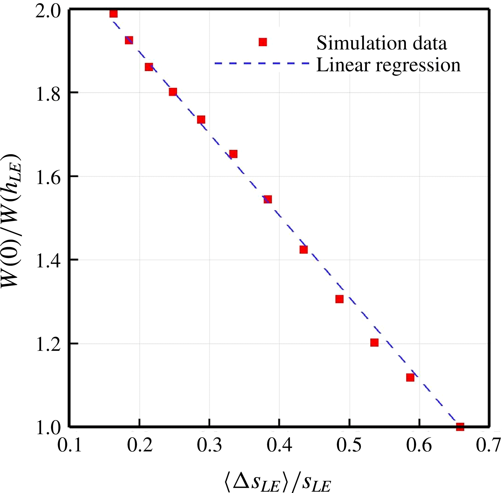
and is plotted in figure 11 as a function of
 $h_{LE}$
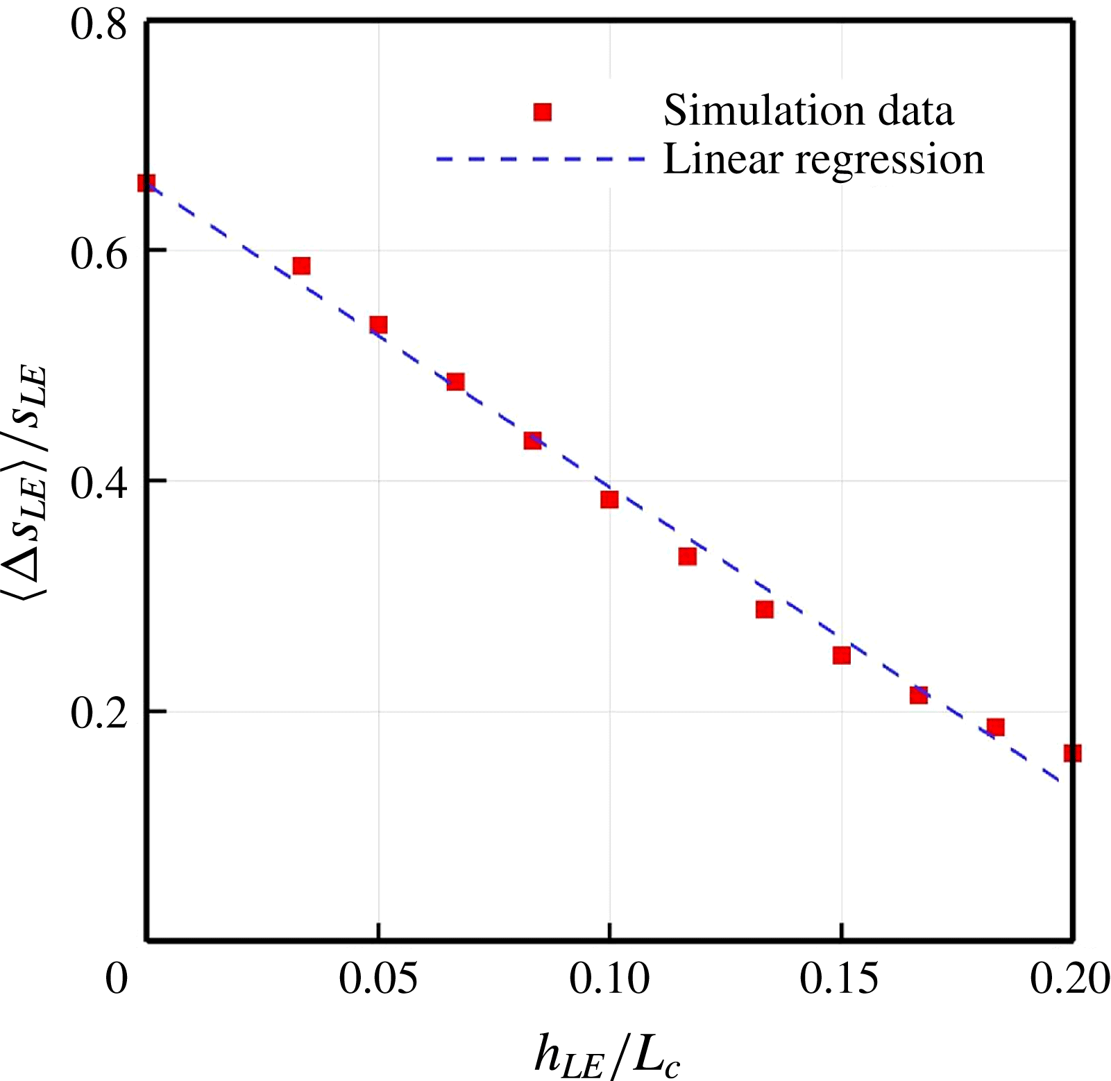
. The figure shows that the edgewise correlation length scale normalised by the full arc length of the WLE (for one period) decreases almost linearly with increasing
 $h_{LE}$
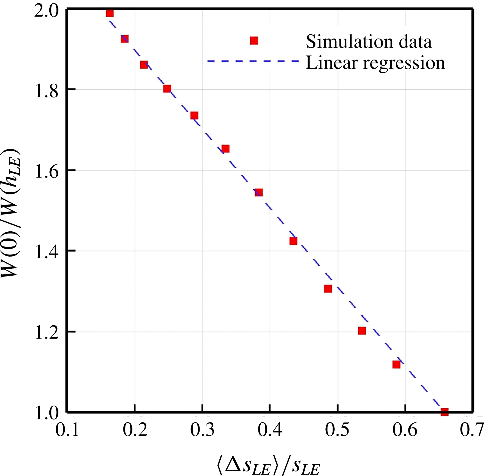
. The results from figures 7 and 11 reveal another linear relation between the noise reduction and the correlation length scale as shown in figure 12.
Normalised correlation length scales of surface pressure fluctuations calculated from (3.7) varying with the amplitude of the WLE profile (
 $h_{LE}$
) for a fixed wavelength (
 ${\it\lambda}_{LE}/L_{c}=2/15$
). The linear regression is
 $y=ax+b$
where
 $a=-2.625$
and
 $b=0.6573$
based on least squares.
To summarise the main findings obtained in this section, the WLE geometry was shown to reduce the ATI noise and the level of noise reduction increases with the amplitude of the WLE sinusoid (
 $h_{LE}$
). One of the possible explanations for this outcome is that the sound source becomes less efficient in the hill region compared to those at the peak and the root as
 $h_{LE}$
increases, due to the effective sweep angle (geometric obliqueness) against the impinging turbulence. Another consequence of increasing
 $h_{LE}$
hence the effective sweep angle is that the correlation of surface pressure fluctuations along the LE (where the most of acoustic energy comes from) becomes weaker and therefore the sound radiation becomes less efficient. Therefore, it may be concluded that the effective sweep angle has a significant impact on the source decorrelation (mainly related to low-frequency responses). It is noteworthy that the level of noise reduction and the correlation length scale of surface pressure fluctuations both exhibit a linear relationship with
 $h_{LE}$
within the current parameter range and problem set-up.
4 ATI noise-reduction mechanisms
It has been shown earlier in figures 4 and 5 that the radiated ATI sound field is significantly attenuated by the use of a WLE. The noise attenuation seems more pronounced in the high-frequency components. The overall pressure fluctuation levels and correlations examined in the previous section are mainly governed by low-frequency components, which are not suitable to fully describe the noise-attenuation event. Therefore, it is required in this section to investigate in detail the mid- to high-frequency contents of the radiated sound as well as those of the surface pressure fluctuations along the LE. In order to examine the frequency contents of the radiated sound, the pressure signals are recorded at an observer point
 $\boldsymbol{x}_{o}=(0,5L_{c},0)$
(see figures 4 and 6) and the sound power spectra are calculated as shown in figure 13. This figure evidences that the noise reduction appears predominantly in the mid- to high-frequencies and the reduction level seems to increase with frequency as was also reported by Narayanan et al. (Reference Narayanan, Chaitanya, Haeri, Joseph, Kim and Polacsek2015). The upper limit of the noise-reduction spectrum and its asymptotic slope (growth rate) particularly varying with the WLE geometry are currently unknown and are a subject of future study. In the meantime, the noise-reduction spectrum shows a number of distinctive frequencies where a local maxima and minima take place, which are listed in table 1. It is suggested towards the end of this section that these frequency components at the far field originate from a phase interference effect existing between the peak and hill regions of the WLE geometry.
Far field: (a) sound power spectra obtained at an observer point
 $\boldsymbol{x}_{o}=(0,5L_{c},0)$
for the SLE and the WLE cases; and, (b) the relative ratio between them in the decibel scale indicating the level of noise reduction. The WLE case is for
 $h_{LE}/L_{c}=1/15$
and
 ${\it\lambda}_{LE}/L_{c}=2/15$
. The non-dimensional frequency
 $f^{\ast }=3$
corresponds to 12 kHz for an aerofoil of
 $L_{c}=15$
cm.

Frequencies at which local maxima and minima take place in the current noise-reduction spectrum (see figure 13).

4.1 Source cutoff effect
An interesting result was observed in figure 14 which shows the contour map of the two-point correlation between the surface pressure fluctuations and the far-field sound pressure. The two-point correlation includes the retarded time (for the sound waves to travel from the surface to the observer) as indicated in (2.13). The contour plot indicates that the radiated sound is significantly less correlated with the source signals at the peak region than those at the root. This was a rather unexpected result because the overall source strengths at the peak and the root were comparable to each other as seen in figures 8 and 9. One of the possible explanations of this finding is that the source signals at the peak region have significantly weaker low-frequency components (but stronger high-frequency components) than those at the root.
Contour plots of two-point correlation
 $R_{p_{s}p_{o}}(\boldsymbol{x}_{s}:\boldsymbol{x}_{o})$
between the surface pressure fluctuations and the radiated far-field sound at an observer point
 $\boldsymbol{x}_{o}=(0,5L_{c},0)$
, for the (a) SLE and (b) WLE cases. The two-point correlation is based on (2.13). The dashed and the dash-dotted lines represent contour lines that enclose the region of
 $R_{p_{s}p_{o}}/p_{\infty }^{2}\geqslant 3\times 10^{-7}$
and
 $R_{p_{s}p_{o}}/p_{\infty }^{2}\leqslant 4\times 10^{-8}$
, respectively.

In order to understand the source characteristics, the power spectra of the surface pressure fluctuations as defined in (2.9) are computed at 9 different probe points along the LE. The exact locations and the labels of the probe points are provided in figure 15, where ‘
 $\text{N}_{0}$
’, ‘
 $\text{N}_{4}$
’ and ‘
 $\text{N}_{8}$
’ denote the peak, hill centre and root, respectively. The computed auto-spectra are plotted in figure 16 comparing the SLE and WLE cases. One of the obvious findings in this figure is that the WLE case has a large variation in the spectra whereas the SLE case has an almost uniform profile, which is consistent with the result shown earlier in figure 8. The power spectra from the WLE case are re-plotted in figure 17 to better understand the source characteristics. It is found that the source strength drops as the probe point moves from the peak towards the hill centre and the level of drop seems to increase with frequency – figure 17(a). The trend completely reverses when the probe points moves further from the hill centre towards the root where the source strength rises – figure 17(c). In this case, the growth in the spectra is rather uniform across all frequencies so that the low-frequency components become significantly higher at the root region than those in the peak and hill regions. Comparing the spectra from the peak and the root, it can be seen that low-frequency components are prevalent at the root but the high-frequency components are stronger at the peak – figure 17(d). This provides a valid answer to the question emerged earlier from figure 14. It is also learnt here that the source spectrum of SLE (averaged over the span) forms an envelope of the two spectra from the peak and the root combined.
Illustration of the current probe points along the LE to obtain time signals of
 ${\rm\Delta}p_{s}^{\prime }$
and calculate the auto- and cross-spectra from the peak (
 $\text{N}_{0}$
) to the root (
 $\text{N}_{8}$
). The actual probe points are located on the second grid line from the LE where the source strength is maximum.

Auto-spectra of surface pressure fluctuations along the LE;
 $S_{p_{s}^{2}}(\boldsymbol{x}_{\text{N}_{i}},f)$
for
 $i=0,\ldots ,8$
; obtained at the probe points denoted in figure 15, for the (a) SLE and (b) WLE cases. The WLE case is for
 $h_{LE}/L_{c}=1/15$
and
 ${\it\lambda}_{LE}/L_{c}=2/15$
.

Investigation of the WLE source characteristics based on the result shown in figure 16.

Above all, the most significant finding in this investigation is that the WLE source around the hill area (compared to those from the peak and the root) becomes almost ineffective across all frequencies and its gap against the SLE source seems increasing with frequency. We believe that this is primarily related to the sweep-angle effect discussed in the previous section. In fact, the reduction of source power from the SLE case to the hill centre shown in figure 17(d) is well predicted by the factor of
 $\cos ^{2}{\it\theta}\sim 0.1$
(an order of magnitude down) where
 ${\it\theta}\sim 72^{\circ }$
at the hill centre according to (3.2a−c
). The diminishing source power in the hill region is suggested as one of the main noise-reduction mechanisms associated with WLE and is herein referred to as a source cutoff effect in this paper. It is expected that some subcritical modes in the flow grazing over the oblique part of the WLE geometry will decay exponentially during their propagation into the far field (hence reinforcing the cutoff event) but they are not distinguished in the surface pressure spectra.
4.2 Source correlation and coherence
We now investigate the source relationships between the peak region and the other remaining regions of the WLE. This investigation is necessary because the noise reduction is dominant at high frequencies as seen in figure 13 (up to 10 dB and over) while the peak region seems to serve as the main source of the high-frequency noise that is as strong as the SLE counterpart – see figure 17(d). It may be hypothesised that a destructive source relationship exists against the peak region so that its strong high-frequency components become inefficient leading to reduced noise. To investigate this, the two-point cross-spectra of the surface pressure fluctuations are computed between the peak (
 $\text{N}_{0}$
) and the remaining probe points (
 $\text{N}_{1},\ldots ,\text{N}_{8}$
). The magnitude of the cross-spectra are plotted in figure 18 comparing the SLE and the WLE cases.
Two-point cross-spectra (magnitude) of surface pressure fluctuations along the LE;
 $\Vert S_{p_{s}p_{s}}(\boldsymbol{x}_{\text{N}_{0}}:\boldsymbol{x}_{\text{N}_{i}},f)\Vert$
for
 $i=1,\ldots ,8$
; between the peak (
 $\text{N}_{0}$
) and the remaining probe points (
 $\text{N}_{1},\ldots ,\text{N}_{8}$
) denoted in figure 15, for the (a,c) SLE and (b,d) WLE cases. The WLE case is for
 $h_{LE}/L_{c}=1/15$
and
 ${\it\lambda}_{LE}/L_{c}=2/15$
.

The result reveals that the overall source correlation level is significantly lower in the WLE case than the SLE in most of the frequency range, which is consistent with the result shown earlier in figure 10. Although the SLE case exhibits a consistent decrease in the correlation level as the gap between the two points grows (from
 $\text{N}_{0}:\text{N}_{1}$
to
 $\text{N}_{0}:\text{N}_{8}$
), the rate of decrease is significantly higher with the WLE up to
 $\text{N}_{0}:\text{N}_{5}$
particularly in the mid- to high-frequency range. The fast decrease seems to cease from
 $\text{N}_{0}:\text{N}_{6}$
to
 $\text{N}_{0}:\text{N}_{8}$
where, by contrast, an increase takes place at low frequencies as observed earlier in the source strength (figure 17).
It is noteworthy in figure 18 that both the SLE and WLE cases show a drop in the cross-spectra at around
 $f^{\ast }=2h_{LE}/u_{\infty }=0.5$
. This is actually due to two different physical phenomena taking place coincidentally at the same frequency in this particular case. First, the frequency is known as the starting frequency at which noticeable noise reduction begins to appear as reported by Narayanan et al. (Reference Narayanan, Chaitanya, Haeri, Joseph, Kim and Polacsek2015). Secondly, the size of eddies in the synthetic turbulence used for the current simulations is mainly between
 $0.1L_{c}$
and
 $0.146L_{c}$
which entirely covers
 $2h_{LE}=0.1333L_{c}$
. It has been checked by the authors that the drop in the spectra splits into two if a different value of
 $h_{LE}$
is chosen or if a different range of the eddy sizes is used.
Relative profiles of the cross-spectra, i.e. the ratio of the WLE ones to the SLE (
 $\Vert S_{p_{s}p_{s}}^{(\text{WLE})}(f)/S_{p_{s}p_{s}}^{(\text{SLE})}(f)\Vert$
) are plotted in figure 19 in order to assess the relative decrease/increase of the source correlation due to the WLE geometry. It is confirmed that the correlation level is constantly lower with WLE at all frequencies for cases up to
 $\text{N}_{0}:\text{N}_{5}$
. However, some high frequencies exhibit significantly increased correlation for cases
 $\text{N}_{0}:\text{N}_{6}$
to
 $\text{N}_{0}:\text{N}_{8}$
. More interestingly, it is possible to relate some of the distinctive frequencies revealed in figure 19 with those listed in table 1. For example, the lowest relative correlation taking place around
 $1.6<f^{\ast }<1.7$
in
 $\text{N}_{0}:\text{N}_{4}$
and
 $\text{N}_{0}:\text{N}_{5}$
may be the cause of the local maximum at
 $f^{\ast }=1.62$
in table 1. Also, the highest relative correlation at
 $f^{\ast }\simeq 1.9$
in
 $\text{N}_{0}:\text{N}_{7}$
coincides with the local minimum of noise reduction at
 $f^{\ast }=1.91$
. However, not all frequencies closely match and it is necessary to study the phase spectra to clarify on these frequencies (to follow in § 4.3).
Relative ratio of the two-point cross-spectra;
 $\Vert S_{p_{s}p_{s}}^{(\mathit{WLE})}(f)/S_{p_{s}p_{s}}^{(\mathit{SLE})}(f)\Vert$
between the WLE and SLE cases; based on the result shown in figure 18.


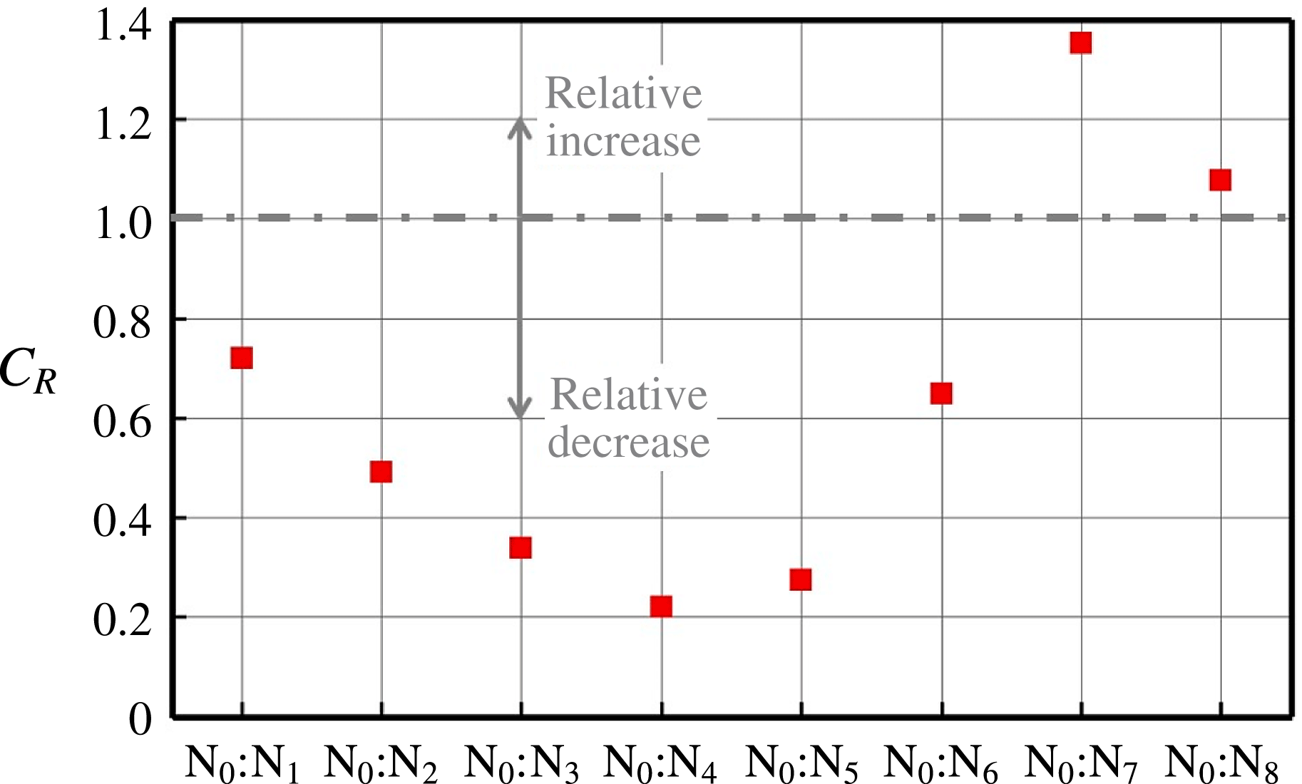
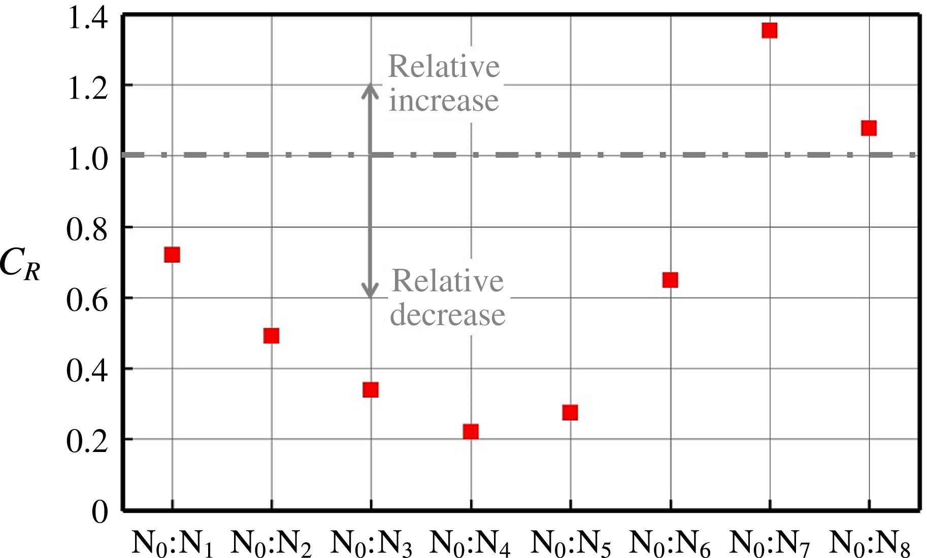
Figure 20 shows the relative decrease/increase of the overall source correlation level due to the geometric modification from SLE to WLE. This is obtained by integrating the profiles of the relative cross-spectra given in figure 19 over a certain frequency range as follows:
 $$\begin{eqnarray}C_{R}(\boldsymbol{x}_{\text{N}_{0}}:\boldsymbol{x}_{\text{N}_{i}})=\frac{1}{f_{b}^{\ast }-f_{a}^{\ast }}\int _{f_{a}^{\ast }}^{f_{b}^{\ast }}\left\Vert \frac{S_{p_{s}p_{s}}^{(\text{WLE})}(\boldsymbol{x}_{\text{N}_{0}}:\boldsymbol{x}_{\text{N}_{i}},f^{\ast })}{S_{p_{s}p_{s}}^{(\text{SLE})}(\boldsymbol{x}_{\text{N}_{0}}:\boldsymbol{x}_{\text{N}_{i}},f^{\ast })}\right\Vert \text{d}f^{\ast }\quad \text{for}~i=1,\ldots ,8.\end{eqnarray}$$
The frequency range of the integration is set to
 $[f_{a}^{\ast },f_{b}^{\ast }]=[0.5,3]$
. The value of
 $f_{a}^{\ast }=0.5$
is chosen here since it has been shown to be the minimum frequency at which significant noise reduction begins to take place as mentioned earlier in § 2.2 – see (2.8). The upper bound
 $f_{b}^{\ast }=3$
is chosen based on the temporal resolution of the signal data available. Figure 20 confirms that the WLE yields a substantial reduction in the source correlation between the peak and hill regions relative to the SLE case. The lowest level takes place at
 $\text{N}_{0}:\text{N}_{4}$
(between the peak and the hill centre). On the other hand, it is observed that the level of source correlation between the peak and root regions (
 $\text{N}_{0}:\text{N}_{7}$
and
 $\text{N}_{0}:\text{N}_{8}$
) may exceed that of the SLE counterpart.
The above investigation based on the two-point cross-spectra has led to some useful information on the source relationships. One of the main findings here is that the source correlation between the peak (
 $\text{N}_{0}$
) and the hill centre (
 $\text{N}_{4}$
) is substantially lower than others. This is perfectly in line with the observation made earlier in § 4.1 where the source strength (auto-spectrum) was found lowest at the hill centre (
 $\text{N}_{4}$
) across all frequencies. Therefore it is possible to reason that the reduced level of the source correlation is mainly due to the low source strength around the hill area (the source cutoff effect) rather than anything else. In order to prove this, the source coherence spectra defined in (2.12) is provided in figure 21 comparing the SLE and WLE cases. It is found from the figure that the coherence level is clearly reduced with WLE in the low-frequency range (
 $f^{\ast }<0.5$
), which evidences the source decorrelation discussed earlier in § 3.2. However, in the mid- to high-frequency range, it is hard to conclude from the coherence spectra that there is an extra source relationship (destructive) in the WLE case leading to a significant noise reduction. The coherence spectra are based on the magnitude of the cross-spectra and their phase relationships are not sufficiently displayed. It is shown below that investigating the phase relationships may be crucial to the understanding of the noise-reduction mechanisms associated with WLEs.
Two-point coherence spectra (magnitude squared) of surface pressure fluctuations along the LE;
 $C_{p_{s}p_{s}}(\boldsymbol{x}_{\text{N}_{0}}:\boldsymbol{x}_{\text{N}_{i}},f)$
for
 $i=1,\ldots ,8$
; between the peak (
 $\text{N}_{0}$
) and the remaining probe points (
 $\text{N}_{1},\ldots ,\text{N}_{8}$
) denoted in figure 15, for the (a) SLE and (b) WLE cases. The WLE case is for
 $h_{LE}/L_{c}=1/15$
and
 ${\it\lambda}_{LE}/L_{c}=2/15$
.

4.3 Phase interference effect
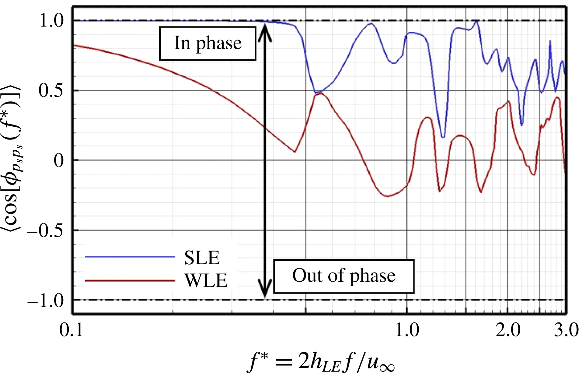
Here we study the phase information of the two-point cross-spectra in order to find and show another type of noise-reduction mechanism – phase interference effect. Figure 22 reveals the phase spectra obtained from (2.12), from which the source phase relationships are investigated. In this figure,
 $\cos ({\it\phi}_{p_{s}p_{s}})$
is plotted instead of the raw phase difference (
 ${\it\phi}_{p_{s}p_{s}}$
) so that the resulting value reaches
 $+1$
when the phase difference is
 $2m{\rm\pi}$
(in phase) and
 $-1$
if it is
 $(2m+1){\rm\pi}$
(out of phase). This is a convenient way of analysing a phase spectrum. It is found in figure 22 that the WLE case exhibits a significantly increased level of phase shifts towards the out-of-phase direction (hence interference) particularly from
 $\text{N}_{0}:\text{N}_{2}$
to
 $\text{N}_{0}:\text{N}_{6}$
compared to the SLE counterpart. Meanwhile, the profiles of the phase spectra becomes increasingly erratic with large oscillations in
 $\text{N}_{0}:\text{N}_{6}$
through to
 $\text{N}_{0}:\text{N}_{8}$
in both the SLE and WLE cases, where qualitatively little distinction can be made. The results indicate that the level of the phase interferences in WLE is significantly promoted between the peak and hill regions compared to that of the SLE case.
The profiles of
 $\cos [{\it\phi}_{p_{s}p_{s}}(\boldsymbol{x}_{\text{N}_{0}}:\boldsymbol{x}_{\text{N}_{i}},f)]$
where
 ${\it\phi}_{p_{s}p_{s}}(\boldsymbol{x}_{\text{N}_{0}}:\boldsymbol{x}_{\text{N}_{i}},f)$
is the two-point phase spectrum of surface pressure fluctuations between the peak (
 $\text{N}_{0}$
) and one of the remaining probe points (
 $\text{N}_{1},\ldots ,\text{N}_{8}$
) denoted in figure 15, for the (a,c) SLE and (b,d) WLE cases. The WLE case is for
 $h_{LE}/L_{c}=1/15$
and
 ${\it\lambda}_{LE}/L_{c}=2/15$
.

The level of the phase interferences may be quantified by taking the average of each profile
 $\cos [{\it\phi}_{p_{s}p_{s}}(\boldsymbol{x}_{\text{N}_{0}}:\boldsymbol{x}_{\text{N}_{i}},f^{\ast })]$
shown in figure 22 over a frequency range:
 $$\begin{eqnarray}C_{{\it\Phi}}(\boldsymbol{x}_{\text{N}_{0}}:\boldsymbol{x}_{\text{N}_{i}})=\frac{1}{f_{b}^{\ast }-f_{a}^{\ast }}\int _{f_{a}^{\ast }}^{f_{b}^{\ast }}\cos [{\it\phi}_{p_{s}p_{s}}(\boldsymbol{x}_{\text{N}_{0}}:\boldsymbol{x}_{\text{N}_{i}},f^{\ast })]\,\text{d}f^{\ast }\quad \text{for}~i=1,\ldots ,8,\end{eqnarray}$$
where the frequency range
 $f^{\ast }\in [f_{a}^{\ast },f_{b}^{\ast }]$
is identical to that of (4.1) as determined earlier. Again, the values of
 $+1$
and
 $-1$
in this measure indicate ‘in-phase’ and ‘out-of-phase’, respectively. The result in figure 23 reveals that the highest level of interference (relative to the SLE case) acting against the source at the peak comes from
 $\text{N}_{3}$
and
 $\text{N}_{4}$
which are positioned around the centre of the hill. This outcome is consistent with the result viewed earlier from figure 20. On the other hand, although the averaged interference levels from
 $\text{N}_{7}$
and
 $\text{N}_{8}$
are relatively unpronounced, they exhibit fully out-of-phase events at a few certain frequencies – see figure 22(c) and (d) – which seem to contribute to shaping the radiated sound spectra as much as those from the other points (
 $\text{N}_{1}$
–
 $\text{N}_{6}$
). In order to examine the overall effects of the phase interference events, the profiles of
 $\cos [{\it\phi}_{p_{s}p_{s}}(\boldsymbol{x}_{\text{N}_{0}}:\boldsymbol{x}_{\text{N}_{i}},f^{\ast })]$
shown in figure 22 are added together and averaged as follows:
 $$\begin{eqnarray}\langle \cos [{\it\phi}_{p_{s}p_{s}}(f^{\ast })]\rangle =\frac{1}{i_{\mathit{max}}}\mathop{X}_{i=1}^{i_{\mathit{max}}}\cos [{\it\phi}_{p_{s}p_{s}}(\boldsymbol{x}_{\text{N}_{0}}:\boldsymbol{x}_{\text{N}_{i}},f^{\ast })],\end{eqnarray}$$
which is then plotted in figure 24 for both the SLE and the WLE cases.
Averaged phase interference levels of surface pressure fluctuations along the LE between the peak (
 $\text{N}_{0}$
) and the remaining probe points (
 $\text{N}_{1},\ldots ,\text{N}_{8}$
) obtained by integrating the profiles shown in figure 22. The definition of
 $C_{{\it\Phi}}$
is given in (4.2).

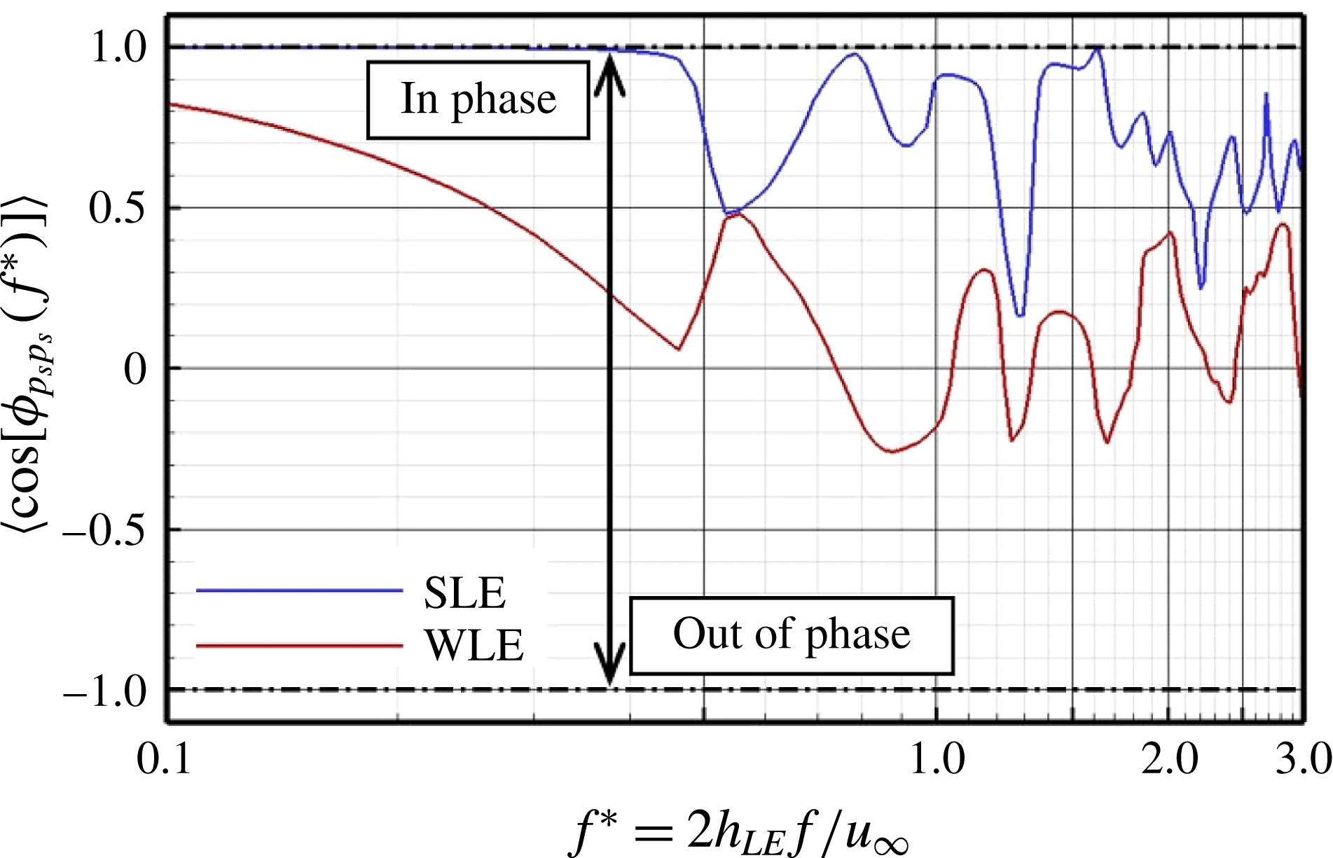
It is evident in figure 24 that the WLE case significantly promotes phase interferences between the peak and the remaining probe points in almost entire frequency range compared to the SLE counterpart. The relative difference of the two averaged phase spectra, i.e.
 ${\rm\Delta}\langle \cos [{\it\phi}_{p_{s}p_{s}}(f^{\ast })]\rangle$
between the SLE and WLE cases is plotted in figure 25(b), which is effectively a spectrum of the phase interference increased due to the modified geometry. This interference spectrum is then compared in figure 25 with the noise-reduction spectrum obtained at the far field (also presented earlier in figure 13). It can be seen from figure 25 that there is a similarity between the two different spectra. It appears that the frequencies at which the local maxima take place (denoted by ‘▵’) match reasonably well between the two spectra. Also the same applies to those of the local minima (denoted by ‘▿’). The agreement seems to be better at higher frequencies except the one near
 $f^{\ast }=2.7$
. The discrepancy near
 $f^{\ast }=2.7$
might be due to the relatively high correlation taking place at that particular frequency (for every LE point) as shown in figure 19. The coincidental sharp increase in the correlation level (despite the large phase interference) might have resulted in a weak noise-reduction effect at that frequency. Meanwhile, the discrepancies in the low-frequency components may be attributed to the fact that there are other mechanisms contributing to the noise reduction (possibly related to vortex dynamics – to be investigated in a follow-on publication). The spectral similarity between the two spectra strongly suggests that the phase interference effect existing between the peak and hill regions of the WLE geometry makes a significant contribution to the reduction of ATI noise.
Relative difference in phase spectra between SLE and WLE cases compared with the radiated noise-reduction spectrum. Symbols denote the local maxima (▵) and minima (▿) of each spectra profile.

5 Concluding remarks
The reduction of ATI noise by using a WLE geometry (with a sinusoidal profile) has been investigated based on high-order accurate compressible Euler simulations with a flat-plate aerofoil. The simulation data offered us a few valuable insights into the understanding of the noise-reduction mechanisms. Firstly, the overall sound pressure level (OASPL) that decreased monotonically (linearly) with the amplitude of the WLE (
 $h_{LE}$
) was related partially with the sweep-angle effect in the hill region where the level of surface pressure fluctuations was substantially lower than those at the peak and the root. The reduction of noise was also related to the rapid decorrelation of surface pressure fluctuations along the LE as
 $h_{LE}$
increased. It was learnt that the edgewise correlation length scale,
 $\langle {\rm\Delta}s_{LE}\rangle$
was a linear function of
 $h_{LE}$
as well (hence, all linear relations between OASPL,
 $\langle {\rm\Delta}s_{LE}\rangle$
and
 $h_{LE}$
) within the current parameter space, which may form a basis to develop a semi-empirical model for the prediction of ATI noise reduction with WLE.
It was found that the noise reduction in the mid- to high-frequency range was contributed by the source cutoff effect taking place mainly in the hill region due to the geometric obliqueness (sweep-angle effect). The source strength diminished rapidly around the hill region across all frequencies. The peak and the root maintained their source strength comparable to that of the SLE counterpart. However, it seemed around the peak region that some of the source power transferred from low frequencies to the high, which might indicate that a nonlinear event took place around the peak region. A follow-on investigation on this is required particularly from fluid dynamic perspectives.
The magnitude-based two-point cross-spectra and coherence spectra led to confirmations on some of the findings in this paper. It was learnt that the source decorrelation was genuinely a low-frequency phenomenon.
The investigation into the phase spectra provided us a significant insight into the understanding of the source relationships, which led to identifying the phase interference effect as one of the mechanisms of ATI noise reduction. The phase interference spectrum at the source (derived in this study) exhibited a noticeable similarity with the noise-reduction spectrum at the far field, showing that the local maxima and minima took place at the same/similar frequencies in both the spectra.
The zero-thickness inviscid flat-plate result offered us useful information to find the fundamental mechanisms. This would be helpful to those who undertake analytical work in which the same assumptions are commonly used. However, the effect of thickness combined with viscosity may be increasingly important when the flow becomes more complex around the WLE geometry (e.g. anisotropic/inhomogeneous turbulence, spanwise skewed mean flow and high incidence angle). It has been briefly shown in the previous experimental paper (Narayanan et al. Reference Narayanan, Chaitanya, Haeri, Joseph, Kim and Polacsek2015) that the level of noise reduction due to WLEs may drop when a thicker aerofoil is used (compared to the flat-plate cases). The level of drop was up to about 2 dB over a wide range of frequencies for the particular aerofoil tested. It is possible that the increased three-dimensionality around the WLE due to the thickness might have played a role there. A comprehensive work plan is required to study and discuss these significant issues.
The current study is based on a low-speed flow as were the cases in the majority of the existing work on WLEs. At present, there are plenty of investigations that should be made in low-speed flows to better understand the physics and mechanisms of WLEs in terms of both aeroacoustics and aerodynamics. In the long term, it is expected that the scope of the work will move towards high-speed flows as well as viscous flows in which more diverse applications can be discussed.
Acknowledgements
The authors gratefully acknowledge the support of EPSRC (Engineering and Physical Sciences Research Council) for the present work under EP/J007633/1. We also acknowledge the high-performance computing facilities and services of the UK National Supercomputer ARCHER via the support of UK Turbulence Consortium (EP/L000261/1) and the local IRIDIS4 at the University of Southampton in the completion of this work.