1. Introduction
In the design of a hypersonic vehicle, knowledge of the factors that affect the thermal and aerodynamic loads acting on the vehicle surface becomes imperative. Usually, in the calculations of the thermal and aerodynamic loads, the analysis assumes that the vehicle has a smooth surface. However, discontinuities or imperfections, such as protuberances, notches, cavities, gaps or steps, are often present on the vehicle surface due to, for instance, fabrication tolerances, sensor installations and differential expansion or ablation rates between non-similar materials (Bertram & Wiggs Reference Bertram and Wiggs1963; Hahn Reference Hahn1969; Nestler, Saydah & Auxer Reference Nestler, Saydah and Auxer1969; Grotowsky & Ballmann Reference Grotowsky and Ballmann2000). Such surface discontinuities or imperfections may constitute a potential source for increased heat flux to the surface, possibly through a premature transition from laminar to turbulent flow.
In hypersonic flight, the flow over protuberances, notches, cavities, gaps or steps may cause local thermal and aerodynamic loads that may dramatically exceed those for a smooth contour. In order to operate safely, these loads have to be predicted correctly. This can be done either by experiments, which are often very expensive for real flight conditions, or by numerical simulation, which is continuously increasing in importance.
An examination of the current literature reveals that much general information is available on the flow physics of protuberances (Bertram & Wiggs Reference Bertram and Wiggs1963; Bertram et al. Reference Bertram, Weinstein, Cary and Arrington1967; Mazaheri & Wood Reference Mazaheri and Wood1967; Estruch et al. Reference Estruch, MacManus, Stollery, Lawson and Garry2010; Neumann & Freeman Reference Neumann and Freeman2012), notches (Charwat Reference Charwat1971; Howell & Korst Reference Howell and Korst1971), cavities (Charwat et al. Reference Charwat, Dewey, Roos and Hitz1961a ,Reference Charwat, Roos, Dewey and Hitz b ; Pan & Acrivos Reference Pan and Acrivos1967; Hahn Reference Hahn1969; Higdon Reference Higdon1985; Morgenstern Jr & Chokani Reference Morgenstern and Chokani1994; Jackson, Hillier & Soltani Reference Jackson, Hillier and Soltani2001; Everhart et al. Reference Everhart, Alter, Merski, Wood and Prabhu2006; Everhart Reference Everhart2009) and gaps (Bertin & Goodrich Reference Bertin and Goodrich1980; Pitts & Murbach Reference Pitts and Murbach1982; Petley et al. Reference Petley, Smith, Edwards, Carlson and Hamilton1984; Vharbonnier & Boerrigter Reference Vharbonnier and Boerrigter1993; Hinderks, Radespiel & Gülhan Reference Hinderks, Radespiel and Gülhan2004; Hinderks & Radespiel Reference Hinderks and Radespiel2006).
For the particular case of steps, there is nowadays a rather extensive literature – mostly, but not entirely, experimental – dealing with forward-facing step flows. In general, these research studies have been conducted in order to understand, among other aspects, the physical aspects of a laminar or turbulent boundary layer in a subsonic (Chapman, Kuehn & Larson Reference Chapman, Kuehn and Larson1958; Stüer, Gyr & Kinzelbach Reference Stüer, Gyr and Kinzelbach1999; Camussi et al.
Reference Camussi, Felli, Pereira, Aloisio and DiMarco2008), supersonic (Bogdonoff & Kepler Reference Bogdonoff and Kepler1955; Chapman et al.
Reference Chapman, Kuehn and Larson1958; Rogers & Berry Reference Rogers, Berry and Leeuw1965; Zukoski Reference Zukoski1967; Uebelhack Reference Uebelhack1969; Driftmyer Reference Driftmyer1973) or hypersonic (Wilkinson & East Reference Wilkinson and East1968; Nestler et al.
Reference Nestler, Saydah and Auxer1969; Pullin & Harvey Reference Pullin and Harvey1977; Grotowsky & Ballmann Reference Grotowsky and Ballmann2000) flow past such a discontinuity, characterized by a sudden change in the surface slope. Certainly, these research studies on forward-facing steps have many useful applications. At low step height to boundary-layer thickness (
 $h/{\it\delta}$
) ratios, the results are important in order to understand and to predict the surface roughness effects on drag and on the performance of aircraft. On the other hand, at larger
 $h/{\it\delta}$
ratios, for instance, the results can be useful for predicting the effectiveness of spoilers and deceleration devices.
Usually, rarefied hypersonic flows are characterized by thick laminar boundary layers. In this fashion, the frontal-face height of steps on the surface of hypersonic vehicles may be less than the boundary-layer thickness. However, specific research studies on heating and pressure loads on forward-facing steps with step heights less than the boundary-layer thickness are very sparse (Rogers & Berry Reference Rogers, Berry and Leeuw1965; Driftmyer Reference Driftmyer1973). For the purpose of this introduction, it will be sufficient to describe only a few of these studies on forward-facing steps.
Bogdonoff & Kepler (Reference Bogdonoff and Kepler1955) conducted an experimental investigation on the separation associated with steps and shock-wave boundary-layer interaction in the continuum flow regime. For a free stream Mach number of approximately three, the experiments showed that separation occurred at a pressure ratio (local static pressure to free stream static pressure) of approximately two for the forward-facing steps investigated. In addition, combined with other investigations, the results indicated a very small variation of the separation pressure ratio with Mach number.
Rogers & Berry (Reference Rogers, Berry and Leeuw1965) conducted an experimental investigation on forward-facing steps in a supersonic flow, Mach number of approximately 2, characterized by a thick laminar boundary layer. The free stream pressure was defined as 30, 50 and
 $70~{\rm\mu}\text{mHg}$
. Eight step heights were tested, ranging in 0.1 in. intervals from 0.1 to 0.9 in., except for 0.8 in. In addition, the step height was comparable with the local boundary-layer thickness for a flat plate without steps. According to the authors, the investigation showed that the largest pressure rise occurred at the step face. Furthermore, it was found that this pressure rise depended on the height-to-length (
 $h/L$
) ratio, where
 $h$
is the step height and
 $L$
is the distance from the flat-plate leading edge to the step position.
Forward-facing steps, for the particular case where the step heights
 $h$
were less that the boundary-layer thickness
 ${\it\delta}$
, were investigated by Driftmyer (Reference Driftmyer1973). The experimental investigation was conducted at a free stream Mach number of 4.9 with a unit Reynolds number in the range of
 $(0.8{-}4.0)\times 10^{6}$
 $\text{ft}^{-1}$
. According to the experimental data, the pressure distributions measured in the separated region ahead of the steps were found to be functions of both
 $\mathit{Re}_{{\it\delta}}$
and
 $h/{\it\delta}$
for the turbulent boundary-layer separation case where
 $h<{\it\delta}$
. It was found that the pressure distribution on the step face was also a function of Reynolds number
 $\mathit{Re}_{{\it\delta}}$
and
 $h/{\it\delta}$
.
Pullin & Harvey (Reference Pullin and Harvey1977) numerically analysed a two-dimensional rarefied hypersonic flow around a forward-facing step by considering
 $\text{N}_{2}$
as the working fluid, and a free stream Mach number of 22. The analysis showed that in the vicinity of the step base, the flow has a rapid deceleration and compression accompanied by a sudden transition to a near-continuum Navier–Stokes-type state nearly in equilibrium at the body temperature. The computational results presented good agreement with experimental data.
Grotowsky & Ballmann (Reference Grotowsky and Ballmann2000) investigated laminar hypersonic flow over forward- and backward-facing steps by employing Navier–Stokes equations. The hypersonic flow over the steps was simulated by considering a free stream Mach number of 8, a Reynolds number of the order of
 $10^{8}$
and an altitude of 30 km. According to them, the computational results presented a good agreement with the experimental data available in the literature. They also pointed out that the quantitative comparison exhibited major differences for the wall heat flux, probably due to the difficulty in measuring it accurately.
The major interest in these studies on forward-facing steps was devoted to considering laminar or turbulent flow in the continuum flow regime. However, there is little understanding of the physical aspects of rarefied hypersonic flows past steps related to the aerothermodynamic environment encountered by re-entry vehicles. In this scenario, the purpose of the present study is to investigate the step-height impact on the flow field structure and on the aerodynamic surface properties of a hypersonic flow on a forward-facing step in the transition flow regime, i.e. between the continuum flow and free collision flow regimes. A detailed and careful effort is made to provide a comprehensive description of the flow with special attention to the particular case where the step height is less than the boundary-layer thickness.
With this aim, the focus of the present study is on the low-density region in the upper atmosphere, where numerical gas kinetic procedures are available to simulate hypersonic flows. At high altitudes, and therefore low density, the molecular collision rate is low and the energy exchange occurs under non-equilibrium conditions. In such circumstances, the Navier–Stokes equations are inappropriate due to the high degree of molecular non-equilibrium. Consequently, the direct simulation Monte Carlo (DSMC) method will be employed to calculate the two-dimensional hypersonic flow on forward-facing steps.
2. Computational tool
Flows are characterized by a variety of dimensionless quantities. The most useful one for the purpose of this work is the Knudsen number
 $\mathit{Kn}$
, defined by the ratio of the molecular mean free path to a characteristic length of the problem. A flow is defined as being in the continuum flow regime when the Knudsen number tends to zero. In this situation, molecules are considered to be so densely packed that the mean free path is insignificant compared with the flow dimensions. On the other hand, a flow is defined as being in the free molecular flow regime as the Knudsen number goes to infinity. Traditionally, the classification of a flow as a function of the Knudsen number is divided into four regimes (Schaff & Chambre Reference Schaff and Chambre1958): (i)
 $\mathit{Kn}<0.01$
, continuum flow, (ii)
 $0.01<\mathit{Kn}<0.1$
, slip flow, (iii)
 $0.1<\mathit{Kn}<10$
, transition flow and (iv)
 $\mathit{Kn}>10$
, free molecular flow.
The choice of the numerical approach to be used to model rarefied non-equilibrium flows greatly relies on the extent of flow rarefaction. For the near-continuum flow regime, it is usually sufficient to take into account the effects of rarefaction through the boundary conditions of slip velocity and temperature jump on the surface. Navier–Stokes equations, commonly used with these boundary conditions, can be derived from the Boltzmann equation by considering the assumption of small deviation of the distribution function from equilibrium. Nevertheless, Navier–Stokes equations become inappropriate for studying rarefied flows where the distribution function becomes considerable in non-equilibrium.
In order to study rarefied flow with a significant degree of non-equilibrium, the DSMC method, pioneered by Bird (Reference Bird1994), has usually been employed. The DSMC method has become the most common computational technique for modelling complex transitional flows of engineering interest.
The DSMC method does not solve a system of equations directly to produce a solution of the flow field, but rather simulates real gas flows with various physical processes by statistically tracking movements and collisions of a large number of simulated particles, each of which is a typical representative of a great number of real gas molecules. Therefore, the DSMC method models the flow as being a collection of discrete particles, each one with a position, velocity and internal energy. The states of particles are stored and modified with time as the particles move, collide and undergo boundary interactions in simulated physical space.
A fundamental assumption in the DSMC method is that the gas is dilute, i.e. the mean molecular diameter is much less than the mean molecular spacing of molecules in the gas. This feature of the DSMC method allows the molecular motion and collisions to be uncoupled over the period of a specific time step. In this fashion, the predictions of the new positions of the molecules as well as the resulting boundary interactions are followed by the selection of a set of possible intermolecular collisions that are appropriate during the time step. In general, the simulation time, discretized into time steps, is identified with the physical time of the real flow, and the time step should be sufficiently small in comparison with the local mean collision time.
The uncoupling of the molecular motion and collisions over small time steps and the division of the flow field into small cells are the key computational assumptions associated with the DSMC method. The method has been tested in the transition flow regime over the last 50 years, and has shown excellent results when compared with experimental data (Harvey Reference Harvey, Moss and Scott1986; Harvey & Gallis Reference Harvey and Gallis2000, Reference Harvey and Gallis2003; Holden & Wadhams Reference Holden and Wadhams2003).
In the present paper, the molecular collision kinetics are modelled by using the variable hard sphere (VHS) molecular model (Bird Reference Bird and Fisher1981), and the no time counter (NTC) collision sampling technique (Bird Reference Bird, Muntz, Weaver and Campbell1989). The VHS model assumes that the cross-section of a molecule changes with the collision energy according to some power law. The exponent is calculated by matching the viscosity of the simulated gas to that of its real counterpart. The VHS model employs the simple hard sphere angular scattering law so that all directions are equally possible for the post-collision velocity in the centre-of-mass frame of reference. However, the collision cross-section depends on the relative speed of colliding molecules.
In the present paper, simulations are performed by using a non-reacting gas model, consisting of
 $\text{N}_{2}$
and
 $\text{O}_{2}$
, while considering energy exchange between translational, rotational and vibrational modes. For diatomic or polyatomic particles, transfer of energy to and from the internal modes has to be considered. Energy exchange between kinetic and internal modes is controlled by the Borgnakke–Larsen statistical model (Borgnakke & Larsen Reference Borgnakke and Larsen1975). The probability of an inelastic collision determines the rate at which energy is transferred between the translational and internal modes after an inelastic collision. For a given collision, the probability is defined by the inverse of the number of relaxation,
 $Z_{R}$
for rotation and
 $Z_{V}$
for vibration, which corresponds to the number of collisions needed, on average, for a molecule to undergo relaxation. In the present paper, the rotational,
 $Z_{R}$
, and vibrational,
 $Z_{V}$
, collision numbers were obtained in a collision-energy-based procedure, as suggested by Boyd (Reference Boyd1998) for rotation and by Bird (Reference Bird and Abe2009) for vibration.
3. Geometry definition
In the present paper, discontinuities on the surface of a hypersonic vehicle are modelled by a forward-facing step. By assuming that the step frontal face
 $h$
is much smaller than the nose radius
 $R$
of a hypersonic vehicle, for instance, the nose radius
 $R$
of a re-entry capsule, i.e.
 $h/R\ll 1$
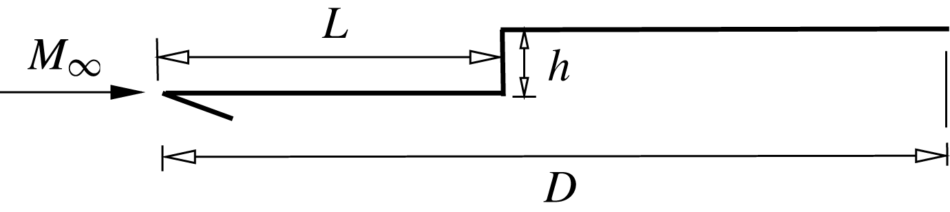
, the hypersonic flow over the step may be considered as a hypersonic flow over a flat plate with a forward-facing step. Figure 1 displays a schematic view of the model employed and presents the important parameters.
A drawing illustrating the forward-facing step schematically.

In figure 1,
 $M_{\infty }$
represents the free stream Mach number,
 $h$
stands for the frontal-face height,
 $L$
is the length of the step upstream surface and
 $D$
is the total length of the flat plate. It was considered that the flat plate was infinitely long but only the total length
 $D$
was examined. Frontal-face heights
 $h$
of 3, 6 and 9 mm were assumed, which correspond to dimensionless face heights
 $H\,(=h/{\it\lambda}_{\infty })$
of 3.23, 6.46 and 9.69 respectively, where
 ${\it\lambda}_{\infty }$
is the free stream mean free path, defined in § 4. In addition, values of
 $L/{\it\lambda}_{\infty }$
of 50 and
 $D/{\it\lambda}_{\infty }$
of 100 were assumed.
An understanding of the impact of the frontal-face height on the flow field structure can be gained by comparing the flow field behaviour of a flat plate with a step with that of a flat plate without a step. In this way, a flat plate free of discontinuities, i.e. without steps, works as a benchmark for the cases with steps, and it will be referred to as the flat-plate case in this work.
4. Free stream and flow conditions
The free stream conditions and gas properties employed in the present calculations are those given by Leite (Reference Leite2009) and tabulated in tables 1 and 2 respectively. These flow conditions represent those experienced by a hypersonic vehicle at an altitude of 70 km. In table 1,
 $T_{\infty }$
,
 $p_{\infty }$
,
 ${\it\rho}_{\infty }$
,
 ${\it\mu}_{\infty }$
,
 $n_{\infty }$
,
 ${\it\lambda}_{\infty }$
and
 $U_{\infty }$
stand respectively for temperature, pressure, density, viscosity, number density, mean free path and velocity. In table 2,
 ${\it\chi}$
,
 $m$
,
 $d$
and
 ${\it\omega}$
stand respectively for mole fraction, molecular mass, molecular diameter and viscosity index.
Free stream flow conditions.

Gas properties.

The free stream velocity
 $U_{\infty }$
, assumed to be constant at
 $7456~\text{m}~\text{s}^{-1}$
, corresponds to a free stream Mach number
 $M_{\infty }$
of 25. The wall temperature
 $T_{w}$
is assumed constant at 880 K.
By assuming the frontal-face height
 $h$
as the characteristic length, the Knudsen number
 $\mathit{Kn}_{h}$
corresponds to 0.3095, 0.1548 and 0.1032 for dimensionless face heights
 $H$
of 3.23, 6.46 and 9.693 respectively. The Reynolds number
 $\mathit{Re}_{h}$
is approximately 136, 272 and 409 for
 $H$
of 3.23, 6.46 and 9.693 respectively, also based on the frontal-face height
 $h$
and on the conditions in the undisturbed stream.
5. Computational flow domain and grid
In order to implement the particle–particle collisions, the flow field around the forward-facing step is divided into an arbitrary number of regions, which are subdivided into quadrilateral cells. The cells are further subdivided into subcells, two subcells per cell in each coordinate direction. The cell provides a convenient reference for the sampling of the macroscopic gas properties, while the collision partners are selected from the same subcell for the establishment of the collision rate. Therefore, the physical space network is used to facilitate the choice of molecules for collisions and for the sampling of the macroscopic flow properties such as density, velocity, pressure, temperature, etc.
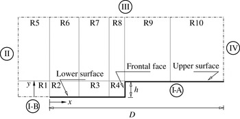
The computational domain used for the calculation is made large enough so that body disturbances do not reach the upstream and side boundaries, where free stream conditions are specified. A schematic view of the computational domain is depicted in figure 2, in which the flow is from the left- to the right-hand side. According to this figure, side I-A is defined by the forward-facing step surface. Diffuse reflection with complete thermal accommodation is the condition applied to this side. In a diffuse reflection, the molecules are reflected equally in all directions, and the final velocity of the molecules is randomly assigned according to a half-range Maxwellian distribution determined by the wall temperature. Side I-B represents a plane of symmetry, where all flow gradients normal to the plane are zero. At the molecular level, this plane is equivalent to a specular reflecting boundary. Sides II and III are the free stream sides through which simulated molecules enter and exit. Side II is positioned
 $5{\it\lambda}_{\infty }$
upstream of the flat-plate leading edge, and side III is defined to be
 $30{\it\lambda}_{\infty }$
,
 $34{\it\lambda}_{\infty }$
and
 $42{\it\lambda}_{\infty }$
above the step upper surface for frontal-face heights
 $H$
of 3.23, 6.46 and 9.69 respectively. In the following, the flow at the downstream outflow boundary, side IV, is predominantly supersonic and vacuum conditions are specified (Guo & Liaw Reference Guo and Liaw2001). Basically, at this boundary, simulated molecules can only exit. Nevertheless, it should be remarked that, close to the wall, molecules may not be moving at supersonic speed. As a result, in this subsonic region close to the wall, there is an interaction between the flow and the downstream boundary. However, the extent of the upstream effect of this boundary condition can be determined by changing the length of the upper surface. For the conditions investigated in the present paper, the upstream disturbance is approximately
 $5{\it\lambda}_{\infty }$
, as can be observed in the results presented for the number flux, pressure and skin friction coefficients in the subsequent sections. Finally, it should be noted that for the purpose of computational modelling, a zero-bluntness leading edge is assumed.
A drawing illustrating the computational domain schematically.

The DSMC results depend on the cell size chosen, the time step and the number of particles per computational cell. In the DSMC code, the linear dimensions of the cells should be small in comparison with the length scale of the macroscopic flow gradients normal to the streamwise directions, which means that the cell dimensions should be of the order of or smaller than the local mean free path (Alexander, Garcia & Alder Reference Alexander, Garcia and Alder1998, Reference Alexander, Garcia and Alder2000). The time step should be chosen to be sufficiently small in comparison with the local mean collision time (Garcia & Wagner Reference Garcia and Wagner2000; Hadjiconstantinou Reference Hadjiconstantinou2000). A very small time step results in an inefficient advancement of the solution and accumulation of statistics. Most particles will take many time steps to cross a given cell. As a result, the collision phase of each time step will involve the same group of particles as the previous time step since almost no particles leave or enter the cell. Moreover, a large time step allows the molecules to move too far without the opportunity to participate in a collision. This again causes a smearing of the properties of the flow, resulting in non-physical results. Therefore, the time step must be chosen such that a typical particle moves approximately one fourth of the cell dimension in each time step. Finally, the number of simulated particles has to be large enough to make statistical correlations between particles insignificant.
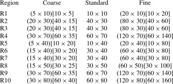
As part of the verification process, a grid independence study was made with three differently structured meshes – coarse, standard and fine – in each coordinate direction. The effect of altering the cell size in the
 $x$
- and
 $y$
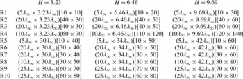
-directions was investigated for the coarse and fine grids with, respectively, 50 % fewer and 100 % more cells with respect to the standard grid. Table 3 summarizes the main characteristics for the standard grid related to ten regions (R1–R10 in figure 2) for cases corresponding to the frontal-face height
 $H$
of 3.23, 6.46 and 9.69. In this way, for
 $H$
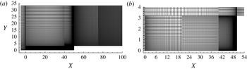
of 3.23, 6.46 and 9.69, the total number of cells corresponds, respectively, to 20 000, 33 800 and 41 600 cells. For completeness, figure 3(a,b) illustrates the standard grid for the
 $H=3.23$
case.
A drawing illustrating the cell distribution for (a) the standard grid for the
 $H=3.23$
case and (b) a magnified view of regions R2, R3 and R4 in the vicinity of the step frontal face.

Dimensions of the regions (
 $x\times y$
) and number of cells [
 $x\times y$
] for
 $H$
of 3.23, 6.46 and 9.69.

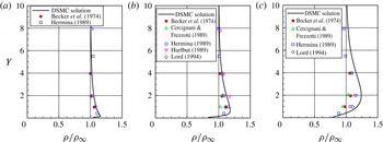
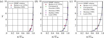
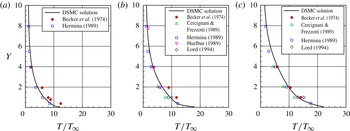
A detailed discussion of the verification process, i.e. the effects of the cell size, time step and number of molecules on the aerodynamic surface quantities for the forward-facing steps presented herein, is given in appendix A. Furthermore, as part of the validation process, results for density, velocity and translational temperature were compared with those obtained from other established DSMC code and experimental data in order to ascertain how well the DSMC code employed in this study is able to predict hypersonic flow about a flat plate. Details of this comparison are also presented in appendix A.
6. Computational results and discussion
Having computed flow field and surface properties over a wide range of simulation parameters, it proves instructive to summarize the major features of the results. Consequently, the purpose of this section is to discuss and compare differences in the flow field properties and the aerodynamic surface properties due to variations in step frontal-face height.
6.1. Flow field properties
This subsection focuses on the calculations of the primary properties obtained from the DSMC results. The primary properties of particular interest in this work are velocity, density, pressure and kinetic temperature.
6.1.1. Velocity field
The DSMC method is essentially a statistical method. In this method, the macroscopic properties are computed as averages from the microscopic properties in each cell in the computational domain. As a result, the velocity vector is given by the following expression:
 $$\begin{eqnarray}\boldsymbol{c}_{0}=\frac{\displaystyle \mathop{\sum }_{j=1}^{N}(m\boldsymbol{c})_{j}}{\displaystyle \mathop{\sum }_{j=1}^{N}m_{j}},\end{eqnarray}$$
where
 $N$
,
 $m$
and
 $\boldsymbol{c}$
represent, respectively, the number of molecules, the molecular mass and the velocity vector of the molecules in each cell. It should be noted that the mean molecular velocity
 $\bar{\boldsymbol{c}}$
(
 $\equiv \boldsymbol{c}_{0}=u\boldsymbol{i}+v\boldsymbol{j}+w\boldsymbol{k}$
) defines the macroscopic mean velocity. It is also important to mention that the velocity of the molecule relative to the mean macroscopic velocity, defined as the thermal or peculiar velocity, is denoted by
 $\boldsymbol{c}^{\prime }\equiv \boldsymbol{c}-\boldsymbol{c}_{0}$
.
Before proceeding with the analysis, it is instructive to first examine the boundary-layer thickness
 ${\it\delta}$
for the flat-plate case, without a step, employed as a benchmark in this investigation. The boundary-layer thickness was obtained by considering the condition
 $u/U_{\infty }=0.99$
, where
 $u$
is the tangential velocity, i.e. the velocity component in the
 $x$
-direction, and
 $U_{\infty }$
is the free stream velocity. It was found that
 ${\it\delta}/{\it\lambda}_{\infty }=16.62$
for a distance of
 $50{\it\lambda}_{\infty }$
from the sharp leading edge. Consequently, the boundary-layer thickness is larger than the step frontal-face height investigated (
 $h/{\it\lambda}_{\infty }$
of 3.23, 6.46 and 9.69), a flow feature of particular interest in this study.
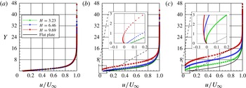
The distribution of tangential velocity
 $u$
for three sections along the lower surface of the steps is illustrated in figure 4(a–c). In this set of plots, the velocity ratio is the tangential velocity
 $u$
normalized by the free stream velocity
 $U_{\infty }$
,
 $H$
is the frontal-face height
 $h$
normalized by the free stream mean free path
 ${\it\lambda}_{\infty }$
,
 $X$
represents the distance
 $x$
from the sharp leading edge, also normalized by
 ${\it\lambda}_{\infty }$
. Therefore, in this framework,
 $X=50$
corresponds to the step position on the flat plate. Finally,
 $Y$
is the distance
 $y$
above the lower surface normalized by
 ${\it\lambda}_{\infty }$
. As a basis of comparison, the tangential velocity profiles for the flat-plate case are illustrated in the same set of plots.
Tangential velocity ratio (
 $u/U_{\infty }$
) profiles for a section
 $X$
of (a) 28, (b) 38 and (c) 48 along the lower surface of the forward-facing step parameterized by the dimensionless frontal-face height
 $H$
.

Important features can be observed in the profiles of tangential velocity shown in this set of plots. For the section
 $X=28$
, the velocity profiles for the step cases are identical, by visual inspection, to those for the flat-plate case. This means that no effect of the presence of the steps is observed up to this section. However, for sections
 $X\geqslant 38$
, the upstream disturbance caused by the steps is observed on the velocity profiles. In addition, it is observed that the velocity profile is affected more upstream with increasing frontal-face height
 $h$
. This behaviour results from the diffusion of molecules that are reflected from the frontal face of the step. Moreover, for sections
 $X\geqslant 38$
, the velocity profiles related to the steps indicate negative velocities near the lower surface, characterizing a recirculation region in the vicinity of the frontal face. For the section
 $X=38$
, negative velocity occurs only for the
 $H=9.69$
case, but for the section
 $X=48$
, all the three frontal-face heights investigated display negative velocities, as shown in figure 4(c). It should be remarked that this flow behaviour, the presence of a recirculation region in the vicinity of a forward-facing step, usually observed in a continuum flow regime (Camussi et al.
Reference Camussi, Felli, Pereira, Aloisio and DiMarco2008), also occurs in a transition flow regime, for the conditions investigated in this work.
Another flow peculiarity with respect to the tangential velocity occurs for
 $Y\approx 0$
, i.e. the velocity along the flat-plate surface, and along the lower surface of the step for sections far from the frontal face. It is clearly seen that
 $u/U_{\infty }\neq 0$
for
 $Y\approx 0$
, a characteristic of a rarefied flow. As a result, the condition of
 $u/U_{\infty }=0$
at the body surface, the no-slip velocity in the continuum flow regime, is not applied in the vicinity of the flat-plate leading edge in a rarefied flow.
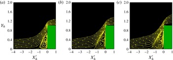
In order to emphasize important features in the flow field structure, streamline traces in the vicinity of the steps are demonstrated in figures 5(a–c). In this group of diagrams,
 $Y_{h}$
stands for the vertical distance
 $y$
, normalized by the step height
 $h$
, and
 $X_{h}^{\prime }$
refers to the horizontal distance (
 $x-L$
), also normalized by the step height
 $h$
. In this context, the reference frame was moved to the step position. According to figures 5(a–c), the presence of a recirculation region is clearly noticed in the vicinity of the frontal face of the steps.
Distribution of streamline traces in the vicinity of the forward-facing step for dimensionless frontal-face heights
 $H$
of (a) 3.23, (b) 6.46 and (c) 9.693.

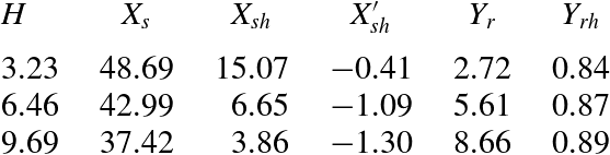
Separation and reattachment points of the flow field as a function of the dimensionless frontal-face height
 $H$
.

The following features are notable in figures 5(a–c). For the
 $H=3.23$
case, the streamlines are basically parallel to the lower surface at section
 $X_{h}^{\prime }=-4.0$
. Therefore, it is thus firmly established that the flow field at sections
 $X_{h}^{\prime }\,\leqslant -4.0$
is unaffected by the presence of the step. In contrast, for the
 $H=6.46$
and 9.69 cases, the streamlines are inclined upward at the same section, an indication that the flow field is affected by the presence of the steps positioned downstream along the lower surface. This information about the presence of the steps is communicated upstream by means of molecular collisions.
Another flow peculiarity is related to the recirculation region. It may be inferred by visual inspection that the recirculation region increases with increasing step height
 $h$
, or by increasing the Reynolds number
 $\mathit{Re}_{h}$
, not only along the lower surface but also along the frontal face. This behaviour differs from that observed in a continuum flow regime. Based on an experimental investigation, Camussi et al. (Reference Camussi, Felli, Pereira, Aloisio and DiMarco2008) pointed out that the separation region occurs independently of the Reynolds number
 $\mathit{Re}_{h}$
. They found that the separation region is of the order of
 $h$
upstream of the step and approximately half of the size of
 $h$
along the frontal face.
Still referring to figures 5(a–c), it is quite apparent that, after the flow separation on the lower surface, the flow reattaches to the frontal face in the vicinity of the step shoulder. Table 4 tabulates the separation point
 $x_{s}$
and the reattachment point
 $y_{r}$
as a function of the dimensionless step height
 $H$
. In this table,
 $X_{s}$
and
 $X_{sh}$
represent, respectively, the separation point
 $x_{s}$
normalized by the free stream mean free path
 ${\it\lambda}_{\infty }$
and by the step height
 $h$
. Moreover,
 $X_{sh}^{\prime }$
corresponds to
 $(x_{s}-L)$
normalized by the step height
 $h$
. Similarly,
 $Y_{r}$
and
 $Y_{rh}$
stand for the point
 $y_{r}$
normalized by
 ${\it\lambda}_{\infty }$
and
 $h$
respectively. According to this table, the results show that the separation point moved away from the step as the step height increased, as observed by Rogers & Berry (Reference Rogers, Berry and Leeuw1965). For the steps under investigation, the separation point
 $x_{s}$
at the lower surface and the reattachment point
 $y_{r}$
on the frontal face were obtained on the basis of zero skin friction coefficient,
 $C_{f}=0$
(or wall shear stress
 ${\it\tau}_{w}=0$
). The reason for this is that the skin friction coefficient along a surface changes from a positive value to a negative value at separation, and vice versa at reattachment, as pointed out by Kim & Setoguchi (Reference Kim and Setoguchi2007) and Deepak, Gai & Neely (Reference Deepak, Gai and Neely2010), and employed by Schäfer, Breuer & Durst (Reference Schäfer, Breuer and Durst2009), Ji & Wang (Reference Ji and Wang2010) and Ji & Wang (Reference Ji and Wang2012). Hence, it is a good indication of the position of separation at the lower surface and reattachment at the frontal face.
6.1.2. Density field
The density in each cell in the computational domain is obtained by the following expression:
 $$\begin{eqnarray}{\it\rho}=\frac{1}{V_{c}}\mathop{\sum }_{j=1}^{N}m_{j},\end{eqnarray}$$
where
 $N$
is the number of molecules in the cell,
 $m$
is the molecular mass and
 $V_{c}$
is the volume of the cell.
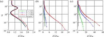
The distribution of density
 ${\it\rho}$
for three sections along the lower surface of the step is displayed in figure 6 parameterized by the dimensionless step height
 $H$
. Similarly to the tangential velocity profiles, the density profiles are shown in this group of plots for three sections defined by
 $X=28$
, 38 and 48. In this group of plots, the density ratio refers to the density
 ${\it\rho}$
normalized by the free stream density
 ${\it\rho}_{\infty }$
. Again,
 $X$
represents the distance
 $x$
, normalized by the free stream mean free path
 ${\it\lambda}_{\infty }$
, and
 $Y$
the distance
 $y$
above the lower surface, also normalized by
 ${\it\lambda}_{\infty }$
. As a basis of comparison, density ratio profiles for the flat-plate case are also presented in the same group of plots. Due to the large range of variation of the ratio
 ${\it\rho}/{\it\rho}_{\infty }$
along the lower surface of the step, the scale in the
 $x$
-direction differs from one plot to another.
Density ratio (
 ${\it\rho}/{\it\rho}_{\infty }$
) profiles for a section
 $X$
of (a) 28, (b) 38 and (c) 48 along the lower surface of the forward-facing step parameterized by the dimensionless frontal-face height
 $H$
.

According to figures 6(a–c), it is clearly seen that the upstream disturbance caused by the step with
 $H=9.69$
is felt by the density profile at section
 $X=38$
. In contrast, there is no indication that the density profile is affected by the presence of the step with
 $H=3.23$
. As expected, by increasing the frontal face
 $h$
, the disturbance caused by the step is felt more upstream in the flow. It should be mentioned in this context that, for
 $X<28$
, the density profiles for the step cases are identical to those for the flat-plate case.
Another flow peculiarity is observed in figures 6(a–c). It is noted that the density increases dramatically as the flow approaches the step, i.e. the density
 ${\it\rho}$
increases by an order of magnitude, almost two, when compared with the free stream density
 ${\it\rho}_{\infty }$
. For comparison purposes, at the step base, the density ratio
 ${\it\rho}/{\it\rho}_{\infty }$
is approximately 32.9, 56.2 and 72.3 for values of
 $H$
of 3.23, 6.46 and 9.69 respectively. This density rise in the vicinity of the frontal face is a characteristic observed in a blunt-body re-entry flow, known as a cold-wall flow. Usually, in a re-entry flow, the wall temperature
 $T_{w}$
is low compared with the stagnation temperature
 $T_{o}$
. For this particular investigation, this ratio is 0.032.
Still referring to figures 6(a–c), it is quite apparent that the density ratio experiences significant changes in the direction perpendicular to the lower surface of the step. For the section
 $X=28$
, the density ratio is high adjacent to the wall,
 $Y\approx 0$
, and rapidly decreases inside a layer with a thickness of approximately one to two free stream mean free paths, where the density ratio is less than one. This means that the density
 ${\it\rho}$
is smaller than the free stream density
 ${\it\rho}_{\infty }$
. After that, as
 $Y$
increases, the density ratio increases significantly at a maximum value,
 ${\it\rho}/{\it\rho}_{\infty }\approx 1.4$
, inside the shock wave. Afterwards, the density decreases again and reaches the free stream density value as
 $Y\rightarrow \infty$
. This behaviour, high-density ratio at the wall and inside the shock wave, and low-density ratio between them, is usually observed when the temperature of the body surface is much lower than the stagnation temperature of the free stream gas. As a result, the gas near the wall tends to be very cold and denser than the rest of the gas in the boundary layer. Furthermore, as will be seen subsequently, the maximum kinetic temperature inside the shock wave takes place in a section corresponding to
 $1<Y<2$
. Consequently, the density decreases in this region, as shown in figure 6(a).
On having a clear qualitative picture of the density behaviour, it becomes instructive to explore the upstream disturbance in the flow due to the presence of the step. A more careful examination was carried out in order to estimate the extent of this effect. In doing so, the difference in the density adjacent the wall was obtained for the two investigations simulated in the present paper, i.e. between the case with a step and the case without a step, the flat-plate case. In this scenario, the
 ${\rm\Delta}{\it\rho}_{x}(={\it\rho}-{\it\rho}_{fp})$
distribution along the lower surface denotes the density rise at section
 $x$
due to the presence of the steps. Figures 7(a,b) illustrate the extension of this effect along the lower surface. In this set of diagrams, the density difference
 ${\rm\Delta}{\it\rho}_{x}$
is normalized by the free stream density
 ${\it\rho}_{\infty }$
. In addition, for illustration purposes, figures 7(a,b) display
 ${\rm\Delta}{\it\rho}_{x}$
as a function of
 $X$
and
 $X_{h}^{\prime }$
respectively, where
 $X_{h}^{\prime }$
refers to the horizontal distance
 $(x-L)$
normalized by the frontal-face height
 $h$
.
The upstream disturbance effect on the density due to the presence of the forward-facing step.

On examining figures 7(a,b), it is observed that the presence of the step causes a significant increase in density in the vicinity of the step. In addition,
 ${\rm\Delta}{\it\rho}_{x}/{\it\rho}_{\infty }$
exhibits a continuous increase up to the frontal face for the
 $H=3.23$
case. Nevertheless, for the
 $H=9.69$
case,
 ${\rm\Delta}{\it\rho}_{x}/{\it\rho}_{\infty }$
exhibits a kink. Moreover, it is clearly noticed that the region affected by the presence of the step is a function of the step height
 $h$
. By considering
 ${\rm\Delta}{\it\rho}_{x}/{\it\rho}_{fp}=0.05$
as the limiting condition, the position corresponding to this condition is denoted as the interaction point,
 $x_{0}$
. In this way, based on the reference system shown in figure 7(a),
 $X_{0}^{\prime }$
corresponds to 38.08, 31.64 and 23.87, for
 $H$
of 3.23, 6.46 and 9.69 respectively. In a similar way, based on figure 7(b), the interaction point
 $X_{0h}^{\prime }$
is approximately
 $-$
3.69,
 $-$
2.84 and
 $-$
2.69 for
 $H$
of 3.23, 6.46 and 9.69 respectively. The difference between the separation point
 $x_{s}$
and the interaction point
 $x_{0}$
determines the pre-separation region, defined here by
 $x_{ps}$
. The pre-separation region defines the distance before the separation that a particular macroscopic property indicates the presence of the step. Table 5 summarizes the interaction point and the pre-separation region related to the density. In this table,
 $X_{0}$
and
 $X_{ps}$
stand, respectively, for the interaction point and the pre-separation region normalized by the free stream mean free path
 ${\it\lambda}_{\infty }$
. Similarly,
 $X_{0h}^{\prime }$
and
 $X_{ps}^{\prime }$
represent the interaction point and the pre-separation region, based on the reference system located at the step position, normalized by the height
 $h$
.
The point of interaction and the pre-separation region related to the density as a function of the dimensionless frontal-face height
 $H$
.

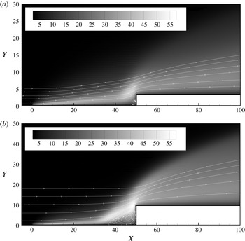
In the following, contour maps along with streamline traces for the density ratio,
 ${\it\rho}/{\it\rho}_{\infty }$
, are displayed in figures 8(a,b) for dimensionless heights
 $H$
of 3.23 and 9.69. The density ratio for the
 $H=6.46$
case is intermediate to the cases shown, and it will not be presented. From this set of plots, as discussed earlier, it is clearly noticed that representative changes in the density ratio take place in the vicinity of the step concave corner.
Contour maps for the density ratio
 $({\it\rho}/{\it\rho}_{\infty })$
for dimensionless frontal-face heights
 $H$
of (a) 3.23 and (b) 9.69.

6.1.3. Pressure field
The pressure in each cell inside the computational domain is obtained by the following equation:
 $$\begin{eqnarray}p=\frac{1}{3V_{c}}\mathop{\sum }_{j=1}^{N}\frac{(mc^{\prime 2})_{j}}{N},\end{eqnarray}$$
where
 $N$
is the number of molecules in the cell,
 $m$
is the molecular mass,
 $V_{c}$
is the volume of the cell and
 $c^{\prime }$
is the thermal velocity of the molecules.
The distribution of pressure
 $p$
for three sections along the lower surface of the step is illustrated in figures 9(a–c) parameterized by the dimensionless step height
 $H$
. In this set of plots, the pressure ratio corresponds to the pressure
 $p$
normalized by the free stream pressure
 $p_{\infty }$
. Here,
 $X$
and
 $Y$
are dimensionless variables as defined previously for the density profiles. Moreover, for comparative purpose, pressure profiles for the flat-plate case are also exhibited in these plots. It is important to emphasize that, due to the large range of variation of the ratio
 $p/p_{\infty }$
along the lower surface of the step, the scale in the
 $x$
-direction differs from one plot to another.
Pressure ratio (
 $p/p_{\infty }$
) profiles for a section
 $X$
of (a) 28, (b) 38 and (c) 48 along the lower surface of the forward-facing step parameterized by the dimensionless frontal-face height
 $H$
.

The upstream disturbance effect on pressure due to the presence of the forward-facing step.

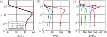
Based on figures 9(a–c), it is noticed that the pressure profiles follow a similar behaviour to that presented by the density profiles in the sense that the pressure profiles for the steps are basically identical to those for the flat-plate case for the section
 $X=28$
, indicating that the pressure field has not been affected yet by the presence of the steps. For the section
 $X=38$
, the pressure field is already affected by the presence of the steps with heights
 $H$
of 6.46 and 9.69. In contrast, no effect is observed in the pressure profile for the section
 $X=38$
due to the presence of the step with a height
 $H$
of 3.23. On the other hand, for the section
 $X=48$
, the pressure profiles for the step cases differ considerably from that for the flat-plate case. As expected, the upstream disturbance increases with increase in the step frontal face. It is also noticed that the pressure ratio increases dramatically as the flow approaches the step base. It is seen that the pressure
 $p$
increases by two orders of magnitude compared with the free stream pressure
 $p_{\infty }$
. For illustration purpose, at the step base, the pressure ratio
 $p/p_{\infty }$
is 142, 230 and 293 for heights
 $H$
of 3.23, 4.46 and 9.69 respectively. Consequently, it may be inferred in passing that particular attention should be paid to the step base in terms of pressure loads, since the vicinity of the step base represents a zone of strong compression.
Proceeding in a manner analogous to the density field, it proves convenient to estimate the upstream disturbance in the pressure field due to the presence of the steps. In this way, the pressure difference
 ${\rm\Delta}p_{x}$
was calculated for the two investigations, i.e. pressure for the flat-plate case with steps minus pressure for the flat-plate case without steps. As calculated along the lower surface, the region defined by
 ${\rm\Delta}p_{x}>0$
represents the pressure rise due to the presence of the steps.
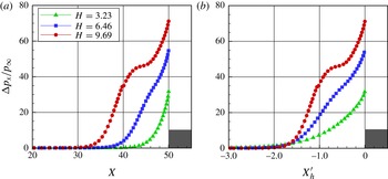
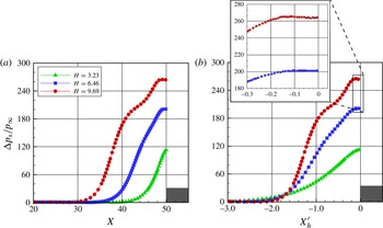
The extension of this effect along the lower surface is displayed in figures 10(a,b). In this group of graphs, the pressure difference
 ${\rm\Delta}p_{x}$
is normalized by the free stream pressure
 $p_{\infty }$
. Besides, for illustration purposes, figures 10(a,b) exhibit
 ${\rm\Delta}p_{x}/p_{\infty }$
as a function of
 $X$
and
 $X_{h}^{\prime }$
, respectively. Based on figures 10(a,b), it is noted that the region affected by the presence of the steps is a function of the frontal-face height. Moreover, it is very encouraging to observe that the pressure difference
 ${\rm\Delta}p_{x}/p_{\infty }$
exhibits a region of constant pressure, a plateau, in the vicinity of the frontal-face base, as highlighted by the magnified view. It should be remarked that the presence of a plateau downstream of the separation point in the pressure profile was reported by Chapman et al. (Reference Chapman, Kuehn and Larson1958). In contrast, Rogers & Berry (Reference Rogers, Berry and Leeuw1965) did not observe any evidence of a constant pressure region. According to these authors, the presence of a plateau might be associated with a high-Reynolds-number phenomenon, which develops when the interaction length is several times the local boundary-layer thickness. For their investigations, the interaction length was relatively small and extended upstream of the steps by two or three boundary-layer thicknesses for the tallest step. For comparison purposes, in the present investigation, the boundary-layer thickness is approximately 1.72 times the tallest step.
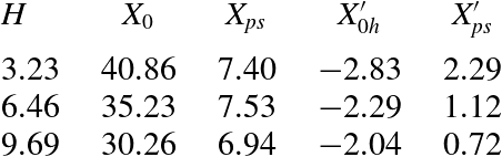
Further, it proves helpful to define the interaction point
 $x_{0}$
and the pre-separation region
 $x_{ps}$
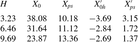
related to the pressure field. Similarly to the density field, these properties were also estimated and are tabulated in table 6. Compared with the data shown in table 5, it is seen that the interaction point and the pre-separation region for the pressure are slightly different from those for the density.
The point of interaction and the pre-separation region related to the pressure as a function of the dimensionless frontal-face height
 $H$
.

Of particular interest is the ratio of the pressure at separation
 $p_{s}$
to the free stream pressure
 $p_{\infty }$
. For
 $H$
values of 3.23, 6.46 and 9.69, the
 $p_{s}/p_{\infty }$
ratio corresponds to 108.8, 116.0 and 125.6 respectively. The dependence of the
 $p_{s}/p_{\infty }$
ratio on the step height was discussed by Bogdonoff & Kepler (Reference Bogdonoff and Kepler1955) for the case of a turbulent boundary layer. For
 $M_{\infty }\approx 3$
, separation occurred at a pressure ratio of approximately 2.1 independently of the step height. By combining their results with other investigations for low Mach numbers, they concluded that the
 $p_{s}/p_{\infty }$
ratio presents a very small change with Mach number. According to Zukoski (Reference Zukoski1967), the
 $p_{s}/p_{\infty }$
ratio is a rather sensitive function of the ratio of step height to boundary-layer thickness as long as
 $h<{\it\delta}$
, but appears to become independent of
 $h/{\it\delta}$
when
 $h>{\it\delta}$
.
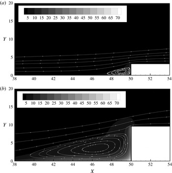
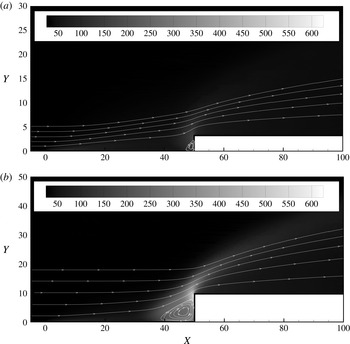
On having a clear qualitative picture of the flow patterns associated with the pressure profiles, it proves convenient to assess the overall performance of the pressure in the entire computational domain. In this way, contour maps along with streamline traces for pressure ratio distributions are demonstrated in figures 11(a,b) for frontal-face heights
 $H$
of 3.23 and 9.69. These plots confirm that the pressure ratio is affected by an increase in the frontal-face height
 $H$
in the vicinity of the steps. In addition, the maximum pressure ratio occurs close to the step shoulder.
Contour maps for the pressure ratio
 $(\,p/p_{\infty })$
for dimensionless frontal-face heights
 $H$
of (a) 3.23 and (b) 9.69.

6.1.4. Kinetic temperature field
In a monatomic gas, the translational temperature, related to the translational kinetic energy of molecules, is simply defined as the temperature. In a diatomic or polyatomic gas, the molecules have internal energy associated with the internal modes of rotation and vibration. In addition, for a gas in thermodynamic equilibrium, the translational temperature is equal to the temperature related to the internal modes, i.e. rotational and vibrational temperatures, and it is identified as the thermodynamic temperature. Conversely, in a thermodynamic non-equilibrium gas, an overall temperature is defined as the weighted mean of the translational and internal temperatures (Bird Reference Bird1994) as
 $$\begin{eqnarray}T_{O}=\frac{{\it\zeta}_{T}T_{T}+{\it\zeta}_{R}T_{R}+{\it\zeta}_{V}T_{V}}{{\it\zeta}_{T}+{\it\zeta}_{R}+{\it\zeta}_{V}},\end{eqnarray}$$
where
 ${\it\zeta}$
is the degree of freedom and the subscripts
 $T$
,
 $R$
and
 $V$
stand for translation, rotation and vibration respectively.
The translational, rotational and vibrational temperatures are obtained for each cell in the computational domain by the following equations:
 $$\begin{eqnarray}\displaystyle & \displaystyle T_{T}=\frac{1}{3k}\mathop{\sum }_{j=1}^{N}\frac{(mc^{\prime 2})_{j}}{N}, & \displaystyle\end{eqnarray}$$
 $$\begin{eqnarray}\displaystyle & \displaystyle T_{R}=\frac{2}{k}\frac{\overline{{\it\varepsilon}_{R}}}{{\it\zeta}_{R}}, & \displaystyle\end{eqnarray}$$
 $$\begin{eqnarray}\displaystyle & \displaystyle T_{V}=\frac{{\rm\Theta}_{V}}{\displaystyle \ln \left(1+\frac{k{\rm\Theta}_{V}}{\overline{{\it\varepsilon}_{V}}}\right)}, & \displaystyle\end{eqnarray}$$
 $k$
is the Boltzmann constant,
 ${\rm\Theta}_{V}$
is the characteristic temperature of vibration and
 $\overline{{\it\varepsilon}_{R}}$
and
 $\overline{{\it\varepsilon}_{V}}$
are, respectively, rotation and vibration average energies in each cell.
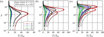
Kinetic temperature profiles along the lower surface are displayed in figures 12(a–c) for sections
 $X$
of 28, 38 and 48 respectively. In this set of diagrams, the temperature ratio stands for the translational temperature
 $T_{T}$
, rotational temperature
 $T_{R}$
, vibrational temperature
 $T_{V}$
or overall temperature
 $T_{O}$
normalized by the free stream temperature
 $T_{\infty }$
. Moreover, the solid lines correspond to the kinetic temperature profiles for the flat-plate case, empty and filled symbols refer to the temperature distributions for frontal-face heights
 $H$
of 3.23 and 9.69 respectively. The temperature profiles for the
 $H=6.46$
case are intermediate to the two other cases, and they will not be shown.
Kinetic temperature ratio (
 $T/T_{\infty }$
) profiles for a section
 $X$
of (a) 28, (b) 38 and (c) 48 along the lower surface of the forward-facing step parameterized by the dimensionless frontal-face height
 $H$
.

On examining figures 12(a–c), it is quite apparent that thermodynamic non-equilibrium occurs throughout the shock layer, as shown by the lack of equilibrium of the translational and internal kinetic temperatures. Thermal non-equilibrium occurs when the temperatures associated with the translational, rotational and vibrational modes of a polyatomic gas are different. The overall kinetic temperature
 $T_{O}$
is equivalent to the thermodynamic temperature only in thermal equilibrium conditions. As a matter of fact, it should be noticed that the ideal gas equation of state does not apply to this temperature in a non-equilibrium situation.
Still referring to figures 12(a–c), it is clearly seen that, in the undisturbed free stream far from the lower surface,
 $Y\rightarrow \infty$
, the translational and internal kinetic temperatures have the same value and are equal to the thermodynamic temperature. On approaching the lower surface, say
 $Y\approx 2$
, the translational kinetic temperature rises to well above the rotational and vibrational temperatures and reaches a maximum value that relies on the section
 $X$
. Since a large number of collisions is needed to excite molecules vibrationally from the ground state to the upper state, the vibrational temperature is seen to increase much more slowly than the rotational temperature. Still further toward the lower surface,
 $Y\approx 0$
, the translational, rotational, vibrational and overall kinetic temperatures decrease, and reach values that depend on the section
 $X$
. For the section
 $X=28$
, the kinetic temperatures reach values on the wall that are above the wall temperature
 $T_{w}$
(
 ${\approx}4T_{\infty }$
), resulting in a temperature jump, as defined in the continuum formulation (Gupta, Scott & Moss Reference Gupta, Scott, Moss and Nelson1985). For the section
 $X=38$
, the difference between the translational temperature and the internal temperatures for the
 $H=9.69$
case indicates that thermodynamic equilibrium is achieved close to the lower surface. Finally, for the section
 $X=48$
, the kinetic temperatures basically reach the wall temperature
 $T_{w}$
, and thermodynamic equilibrium is achieved for the cases defined by
 $H$
values of 3.23 and 9.69.
In order to bring out the essential features of the temperature field, contour maps along with streamline traces for the overall temperature ratio,
 $T_{O}/T_{\infty }$
, are depicted in figures 13(a,b) for dimensionless heights
 $H$
of 3.23 and 9.69.
Contour maps for the overall temperature ratio (
 $T_{O}/T_{\infty }$
) for dimensionless frontal-face heights
 $H$
of (a) 3.23 and (b) 9.69.

Having completed the discussion of the flow field structure, attention is now turned to the aerodynamic properties, where the basic idea is to provide a comprehensive discussion of the results related to the surface quantities, with special attention to the heating and pressure loads.
6.2. Aerodynamic surface properties
The aerodynamic surface quantities of particular interest in the present paper are the number flux, pressure, shear stress and heat transfer. Thus, the purpose of this subsection is to present and discuss these quantities, expressed in coefficient form, with variation in the step frontal-face height.
6.2.1. Number flux
The number flux
 $N$
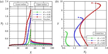
is calculated by sampling the molecules impinging on the surface by unit time and unit area. The distribution of the number flux along the step surfaces – lower, face and upper – is illustrated in figures 14(a,b). In this group of plots,
 $N_{f}$
represents the number flux
 $N$
normalized by
 $n_{\infty }U_{\infty }$
, where
 $n_{\infty }$
is the free stream number density and
 $U_{\infty }$
is the free stream velocity. In addition,
 $X$
and
 $Y$
are the lengths
 $x$
and
 $y$
normalized by the free stream mean free path
 ${\it\lambda}_{\infty }$
. As a basis of comparison, the dimensionless number flux for the flat-plate case is also illustrated in these plots.
The distribution of the number flux
 $N_{f}$
along (a) the lower and upper surfaces and (b) the frontal-face surface parameterized by the dimensionless frontal-face height
 $H$
.

Looking first at figure 14(a), it is clearly noticed that the number flux to the surface depends on the frontal-face height
 $H$
. Close to the sharp leading edge, the behaviour of the number flux to the step lower surface is similar to that for the flat-plate case. This is an expected behaviour since the flow in this region is not affected by the presence of the step. As the flow develops downstream along the lower surface, the presence of the step is felt in the number-flux distribution at section
 $X$
corresponding to approximately 32.6, 38.1 and 43.4 for frontal-face heights
 $H$
of 9.69, 6.46 and 3.23 respectively. From these sections up to the section where the steps are located (
 $X=50$
) the number flux to the lower surface increases dramatically in comparison with the number flux observed for the flat-plate case.
Of particular interest is the number-flux behaviour in the vicinity of the step base. This region, where a significant number-flux rise is observed, is directly related to the recirculation zone that forms ahead of the step frontal face. The recirculation zone concentrates a large number of molecules. The molecules enclosed in this region, when colliding with the lower and frontal-face surfaces, increase not only the number flux to both surfaces but also the energy exchange as well as the linear momentum.
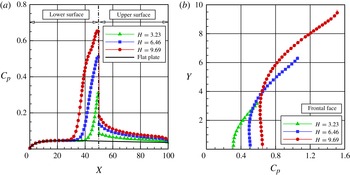
The distribution of the pressure coefficient
 $C_{p}$
along (a) the lower and upper surfaces and (b) the frontal-face surface parameterized by the dimensionless frontal-face height
 $H$
.

Turning next to figure 14(b), it can be seen that the number flux to the frontal-face surface is more intense than that observed to the lower surface. Similarly to that for the lower surface, the number flux to the frontal face is a function of the step height
 $H$
, i.e. it increases with increase of the frontal-face height. It may be recognized from this figure that the number-flux distribution presents a peak value in the vicinity of the step corner. It should be remarked that the peak value occurs at section
 $Y$
equal to 2.79, 6.03 and 9.16 for
 $H$
of 3.23, 6.46 and 9.69 respectively. As a matter of fact, the flow reattachment point,
 $Y_{r}$
, on the frontal face occurs for section
 $Y$
equal to 2.72, 5.61 and 8.66 for
 $H$
of 3.23, 6.46 and 9.69 respectively.
6.2.2. Pressure coefficient
The pressure coefficient
 $C_{p}$
is defined as follows:
 $$\begin{eqnarray}C_{p}=\frac{p_{w}-p_{\infty }}{{\textstyle \frac{1}{2}}{\it\rho}_{\infty }U_{\infty }^{2}}.\end{eqnarray}$$
The pressure
 $p_{w}$
on the body surface is calculated by the sum of the normal momentum fluxes of both incident and reflected molecules at each time step as follows:
 $$\begin{eqnarray}p_{w}=p_{i}-p_{r}=\frac{F_{N}}{A{\rm\Delta}t}\mathop{\sum }_{j=1}^{N}\{[(mv)_{j}]_{i}-[(mv)_{j}]_{r}\},\end{eqnarray}$$
where
 $F_{N}$
is the number of real molecules represented by a single simulated molecule,
 $N$
is the number of molecules colliding with the surface by unit time and unit area,
 ${\rm\Delta}t$
refers to the time step,
 $A$
is the reference area,
 $m$
is the molecular mass and
 $v$
is the velocity component of the molecule
 $j$
in the surface normal direction.
The impact on the pressure coefficient
 $C_{p}$
due to changes in the frontal-face height
 $h$
is depicted in figures 15(a,b) for the lower, frontal-face and upper surfaces. From this group of plots, it is noted that the pressure coefficient behaviour follows the same trend as that shown for the number flux in the sense that (i) the pressure coefficient behaviour along the step surface is similar to that for the flat-plate case in the vicinity of the sharp leading edge, (ii) the upstream disturbances in the pressure coefficient
 $C_{p}$
, due to the presence of the step, are felt up to section
 $X$
corresponding to approximately 32.6, 38.1 and 43.4 for steps with heights
 $H$
of 9.69, 6.46 and 3.23 respectively, (iii) from these sections to the step position, the pressure coefficient
 $C_{p}$
increases dramatically when compared with that for the flat-plate case, (iv) the maximum values for the pressure coefficient
 $C_{p}$
along the lower surface occur at the stagnation point, at the lower-surface/frontal-face junction, (v) along the frontal-face surface, the peak value for
 $C_{p}$
occurs close to the frontal-face/upper-surface junction.
For comparison purposes, the maximum values for
 $C_{p}$
on the frontal face are approximately 0.61, 1.06 and 1.51 for heights
 $H$
of 3.23, 6.46 and 9.69 respectively. In contrast, the maximum value of
 $C_{p}$
for the flat-plate case, i.e. a flat plate without steps, is approximately 0.0471 at section
 $X=25.57$
on the lower surface. Therefore,
 $C_{p}$
values of 0.61, 1.06 and 1.51 correspond respectively to 12.95, 22.52 and 32.06 times the peak value for the flat-plate case, which corresponds to a smoothsurface.
It is noteworthy that, similarly to the number flux, the pressure coefficient rise in the vicinity of the frontal face is directly related to the recirculation zone that forms ahead of the step. This pressure rise is explained by the fact that molecules, confined in the recirculation zone, collide with the lower surface and with the frontal face of the step, resulting in an increase in the normal momentum to both surfaces of the step.
6.2.3. Skin friction coefficient
The skin friction coefficient
 $C_{f}$
is defined as follows:
 $$\begin{eqnarray}C_{f}=\frac{{\it\tau}_{w}}{{\textstyle \frac{1}{2}}{\it\rho}_{\infty }U_{\infty }^{2}}.\end{eqnarray}$$
The shear stress
 ${\it\tau}_{w}$
on the body surface is calculated as the sum of the tangential momentum fluxes of both incident and reflected molecules impinging on the surface at each time step by the following expression:
 $$\begin{eqnarray}{\it\tau}_{w}={\it\tau}_{i}-{\it\tau}_{r}=\frac{F_{N}}{A{\rm\Delta}t}\mathop{\sum }_{j=1}^{N}\{[(mu)_{j}]_{i}-[(mu)_{j}]_{r}\},\end{eqnarray}$$
where
 $u$
is the velocity component of the molecule
 $j$
in the surface tangential direction.
It is worthwhile to note that for the special case of diffuse reflection, the gas–surface interaction model adopted herein, the reflected molecules have a tangential momentum equal to zero, since molecules essentially lose, on average, their tangential velocity components. Thus, the tangential momentum flux of the molecules is defined as follows:
 $$\begin{eqnarray}{\it\tau}_{w}={\it\tau}_{i}=\frac{F_{N}}{A{\rm\Delta}t}\mathop{\sum }_{j=1}^{N}\{[(mu)_{j}]_{i}\}.\end{eqnarray}$$
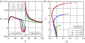
The distribution of the skin friction coefficient
 $C_{f}$
along the step surfaces – lower, frontal face and upper – is displayed in figures 16(a,b). Once again, in this set of plots,
 $X$
and
 $Y$
represent, respectively, the lengths
 $x$
and
 $y$
normalized by the free stream mean free path
 ${\it\lambda}_{\infty }$
.
The distribution of the skin friction coefficient
 $C_{f}$
along (a) the lower and upper surfaces and (b) the frontal-face surface parameterized by the dimensionless frontal-face height
 $H$
.

Looking first at figure 16(a), it is observed that the upstream disturbances, due to the presence of the steps, are felt in the skin friction coefficient
 $C_{f}$
approximately up to sections
 $X$
of 32.6, 38.1 and 43.4 for heights
 $H$
of 9.69, 6.46 and 3.23 respectively. From this position to the step position, the skin friction coefficient
 $C_{f}$
decreases, when compared with that for the flat-plate case, and reaches zero for sections
 $X$
of 37.4, 42.9 and 48.6 for heights
 $H$
of 9.69, 6.46 and 3.23 respectively. After that, as a result of the recirculation region, the skin friction coefficient
 $C_{f}$
continues to decrease until a minimum value that depends on the step height
 $h$
. After the minimum value,
 $C_{f}$
increases again and reaches positive values close to the stagnation point at the base of the step. Along the upper surface, the skin friction coefficient
 $C_{f}$
presents the maximum value at the step shoulder, then drops off downstream and approaches the value observed for the flat-plate case.
Turning to figure 16(b), along the frontal face, the skin friction coefficient
 $C_{f}$
is basically zero at the step base. After that, it stays negative from the step base up to the flow reattachment point. From this point up to the step corner, the skin friction coefficient increases drastically, since this is basically a region exposed to a high-speed flow. Afterwards, due to the flow expansion around the step corner, the skin friction coefficient
 $C_{f}$
diminishes by approximately 50 % in comparison to the values observed at the beginning of the upper surface. It should be emphasized that the section corresponding to the condition of
 $C_{f}=0$
was used to define the separation and reattachment points. As mentioned earlier, the skin friction coefficient along a surface changes from a positive value to a negative value at separation and vice versa at reattachment (Kim & Setoguchi Reference Kim and Setoguchi2007; Deepak et al.
Reference Deepak, Gai and Neely2010). Therefore, it is a good indication of the position of separation at the lower surface and reattachment at the frontal face.
A more careful analysis of the distribution of the skin friction coefficient
 $C_{f}$
reveals important flow peculiarities in the vicinity of the step base. As shown in figure 16(a), the skin friction coefficient
 $C_{f}$
, after reaching the maximum negative value, increases again and reaches positive values in the vicinity of the stagnation point. A magnified view of the stagnation region indicates that the skin friction coefficient
 $C_{f}$
becomes positive in this region, more precisely at sections
 $X$
of 49.1, 49.3 and 49.1 for heights
 $H$
of 3.23, 6.46 and 9.69 respectively. Therefore, the skin friction coefficient starts with positive values near the sharp leading edge, becomes negative along the lower surface, then changes to positive values very close to the stagnation point. It should be emphasized that the change from positive to negative value of the skin friction coefficient
 $C_{f}$
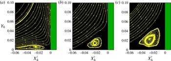
indicates a change in the flow direction, and results in a recirculation region as shown in figures 5(a–c). Consequently, a new sign change, from a negative to a positive value, may indicate the possibility of a second recirculation region very close to the step base. In attempting to assess this effect, a magnified view of figures 5(a–c) was obtained in the vicinity of the step base. This magnified view revealed the formation of a second recirculation region in a much smaller scale than that shown previously in figures 5(a–c).
For completeness, figures 17(a–c) illustrate this second recirculation zone very close to the step base. In this group of plots,
 $Y_{h}$
represents the vertical distance
 $y$
normalized by the frontal-face height
 $h$
, and
 $X_{h}^{\prime }$
refers to the horizontal distance
 $(x-L)$
also normalized by the height
 $h$
. From this set of plots it is very encouraging to observe that, for the conditions investigated in this work, a second recirculation region appears between the first recirculation region and the step base, i.e. in the concave step corner.
The distribution of the streamline traces in the vicinity of the step base for dimensionless frontal-face heights
 $H$
of (a) 3.23, (b) 6.46 and (c) 9.69.

This second recirculation region is a very small region for the
 $H=3.23$
case, increases for the
 $H=6.46$
case and becomes a well defined region for the
 $H=9.69$
case. Of particular interest is the flow direction in both recirculation regions. The flow in the first recirculation region turns in the clockwise direction, whereas the flow in the second recirculation region turns in the counterclockwise direction. Moreover, it should be emphasized that the second recirculation region is formed by molecules with low velocity. On the other hand, it is a region with a high concentration of molecules. As a basis of comparison, for step heights
 $H$
of 3.23, 6.46 and 9.69, the density
 ${\it\rho}$
is, respectively, approximately 32.9, 56.2 and 72.3 times the free stream density
 ${\it\rho}_{\infty }$
at the step base, as mentioned previously. Confined in this region, some of these molecules collide with the lower surface, exchanging energy and linear momentum. Back in the recirculation region, these molecules collide with the step frontal face, again exchanging energy and linear momentum. As a result, a large flux of molecules to both walls is observed in the vicinity of the step base, as indicated in figures 14(a,b).
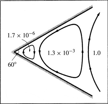
It is important to recall that the presence of a second recirculation region is consistent with the findings of Moffatt (Reference Moffatt1964) in the sense that it is possible to induce a flow near a corner simply by stirring a distant fluid. Under certain conditions, the flow sufficiently near the corner consists of a sequence of eddies of decreasing size and rapidly decreasing intensity, as shown in figure 18. The dimensions of successive eddies fall off in geometric progression with a ratio of
 $r_{n}/r_{n+1}\approx 16.28$
for a corner with a right angle, where
 $r_{n}$
and
 $r_{n+1}$
are the distances of the centres of the
 $n$
th and (
 $n+1$
)th eddies from the corner respectively. As a basis of comparison, the ratio of the sizes of the first and second recirculation regions found in this investigation is approximately 12.6 for the
 $H=9.69$
case. Therefore, this value is in reasonable agreement with the theoretical value calculated by Moffatt (Reference Moffatt1964).
A drawing illustrating Moffatt eddies in a 60° concave corner. The values indicate the relative intensities (adapted from Moffatt (Reference Moffatt1964)).

It is perhaps worth noting that, based on an analytical work, Moffatt derived an expression for the complex stream function as a function of the angle
 $2{\it\alpha}$
between two rigid boundaries for the flow in the vicinity of sharp corners. Under the condition
 $2{\it\alpha}<146^{\circ }$
, Moffatt (Reference Moffatt1964) showed the existence of an infinite sequence of closed eddies with decreasing size and strength in the sharp corner (see figure 18), known as Moffatt eddies. On the other hand, for angles above the critical value,
 $2{\it\alpha}>146^{\circ }$
, no Moffatt eddies are observed. Indeed, it is quite apparent that an infinite system of vortices due only to the viscosity effect is unexpected because of its dissipative role. In addition, it is somewhat surprising with the disappearance of these vortices for
 $2{\it\alpha}>146^{\circ }$
. This problem was defined as Moffatt’s paradox (Goldshtik Reference Goldshtik1990).
6.2.4. Heat transfer coefficient
The heat transfer coefficient
 $C_{h}$
is defined as follows:
 $$\begin{eqnarray}C_{h}=\frac{q_{w}}{{\textstyle \frac{1}{2}}{\it\rho}_{\infty }U_{\infty }^{3}}.\end{eqnarray}$$
The heat flux
 $q_{w}$
to the body surface is calculated by the net energy flux of the molecules impinging on the surface. A flux is regarded as positive if it is directed toward the body surface. The net heat flux
 $q_{w}$
is related to the sum of the translational, rotational and vibrational energies of both incident and reflected molecules, as defined by
 $$\begin{eqnarray}q_{w}=q_{i}-q_{r}=\frac{F_{N}}{A{\rm\Delta}t}\left\{\mathop{\sum }_{j=1}^{N}\left[\frac{1}{2}m_{j}c_{j}^{2}+e_{Rj}+e_{Vj}\right]_{i}-\mathop{\sum }_{j=1}^{N}\left[\frac{1}{2}m_{j}c_{j}^{2}+e_{Rj}+e_{Vj}\right]_{r}\right\},\end{eqnarray}$$
where
 $F_{N}$
is the number of real molecules represented by a single simulated molecule,
 $N$
is the number of molecules colliding with the surface by unit time and unit area,
 ${\rm\Delta}t$
refers to the time step,
 $A$
is the area,
 $m$
is the molecular mass,
 $c$
is the velocity of the molecules and
 $e_{R}$
and
 $e_{V}$
stand for the rotational and vibrational energies respectively. The subscripts
 $i$
and
 $r$
refer to incident and reflected molecules.
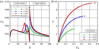
The dependence of the heat transfer coefficient
 $C_{h}$
on the frontal-face height
 $h$
is demonstrated in figures 19(a,b) for the lower, frontal face and upper surfaces. According to this set of diagrams, important features can be observed in the heat transfer coefficient behaviour. For instance: (i) Similarly to the number flux, the heat transfer coefficient
 $C_{h}$
for forward-facing steps follows the same behaviour as that presented by the flat-plate case close to the sharp leading edge; that is, the region unaffected by the presence of the steps. (ii) Further downstream along the lower surface, the heat transfer coefficient
 $C_{h}$
increases significantly and reaches peak values close to the frontal face, then decreases to almost zero in the stagnation region. (iii) Along the upper surface, the heat transfer coefficient presents a maximum value at the step corner and then decreases downstream along the surface, basically approaching the values observed for the flat-plate case. (iv) Along the frontal face, the heat transfer coefficient increases monotonically, from zero at the stagnation point to a maximum value near the step corner, which depends on the frontal-face height
 $h$
. (v) It is quite apparent that this significant increase in the heat transfer coefficient is due to the flow reattachment zone. (vi) Finally, the maximum values observed for the heat transfer coefficient on the frontal-face surface are an order of magnitude larger than those observed on the lower surface. For comparative purposes, the maximum values for
 $C_{h}$
are approximately 0.20, 0.33 and 0.47 for heights
 $H$
of 3.23, 6.46 and 9.69 respectively. In contrast, the
 $C_{h}$
for the flat-plate case, i.e. a flat plate without steps, is approximately 0.031 at section
 $X=8.62$
in the lower surface. Therefore,
 $C_{h}$
values of 0.20, 0.33 and 0.47 correspond respectively to 6.45, 10.65 and 15.16 times the peak value for the flat-plate case.
The distribution of the heat transfer coefficient
 $C_{h}$
along (a) the lower and upper surfaces and (b) the frontal-face surface parameterized by the dimensionless frontal-face height
 $H$
.

Another feature of particular interest in the heat transfer coefficient behaviour is related to the peak values on the lower surface due to the presence of the step in the flow. As shown in figure 19(a), the maximum values observed for the heat transfer coefficient
 $C_{h}$
as well as the locations at which they occur depend on the frontal-face height
 $H$
. For heights
 $H$
of 3.23, 6.46 and 9.69, the maximum values for the heat transfer coefficient
 $C_{h}$
correspond to sections
 $X$
of 47.5, 42.8 and 37.1 respectively. Nevertheless, the separation point corresponds to sections
 $X_{s}$
of 48.69, 42.99 and 37.42 for
 $H$
values of 3.23, 6.46 and 9.69 respectively. Therefore, it is thus firmly established that the point of maximum heat flux to the lower surface basically coincides with the separation point. For the time being, it is worth taking a closer look at the peak values for the
 $H=9.69$
case. Referring to figure 19(a), a second point of maximum heat transfer coefficient is clearly noticed in the vicinity of the concave step corner, more precisely for a section of
 $X=46.5$
. This behaviour differs from the other two cases, i.e. frontal-face heights
 $H$
of 3.23 and 6.46.
A detailed and careful effort was made in order to identify the physical process responsible for this second peak for the heat transfer coefficient
 $C_{h}$
. According to (6.13) and (6.14), the heat transfer coefficient can be separated into two parts: one part related to the contribution of the incident energy and the other one to the contribution of the reflected energy from the surface of the step. Thus, figures 20(a–c) demonstrate the distribution of these two contributions along the lower surface for heights
 $H$
of 3.23, 6.46 and 9.69. In this set of plots,
 $C_{hi},C_{hr}$
and
 $C_{h}$
correspond, respectively, to the incident, reflected and total heat transfer coefficients.
The distribution of the incident, reflected and total heat transfer coefficients along the lower surface of the step with height
 $H$
of (a) 3.23, (b) 6.46, and (c) 9.69.

From figures 20(a–c), it is clearly seen that the maximum point in the heat transfer coefficient distribution is directly related to the incident heat flux to the surface of the step. One can also recognize from these plots the presence of one peak value in the incident distribution
 $C_{hi}$
for the
 $H=3.23$
case and two peak values for the
 $H=9.69$
case. For the intermediate case,
 $H=6.46$
, it is also seen that one peak value occurs in the
 $C_{hi}$
distribution; however, there is sufficient evidence of the formation of a second peak value. It should be remarked that the incident heat flux
 $C_{hi}$
to the surface is composed of the contributions of the translation, rotation and vibration energies of the molecules, as defined in (6.9). In this sense, figures 21(a–c) display the contributions of each energy mode along the lower surface for the heights
 $H$
of 3.23, 6.46 and 9.69 respectively. In this group of diagrams, the subscripts
 $T,R$
and
 $V$
refer, respectively, to translation, rotation and vibration energy modes of the molecules.
The contribution of translation, rotation and vibration energy modes to the incident heat transfer coefficient along the lower surface of the step with height
 $H$
of (a) 3.23, (b) 6.46 and (c) 9.69.

Referring to figures 21(a–c), it is firmly established that the three energy modes contribute to the formation of the peak values in the heat transfer distribution to the lower surface. It is seen that the translation energy contributes the largest portion, followed by the rotation and, finally, the vibration energy. Nevertheless, there is no evidence that a particular internal energy mode is responsible for the second peak value in the heat transfer coefficient for the
 $H=9.69$
case. Thus, the physical process, related to the presence of the peak values in the heat transfer coefficient at sections of
 $X=47.5$
, 42.8 and 37.1, can be explained as follows. As shown earlier, the location of the peaks corresponds to the recirculation zone. Some of the molecules confined in the recirculation zone collide with the frontal-face surface of the step. These molecules exchange energy with the frontal-face surface (see figure 19
b) and reflect from the surface with an energy corresponding to the step surface temperature
 $T_{w}$
. Back in the recirculation zone, in a clockwise direction (see figures 5
a–c), some of these molecules collide with the lower surface and exchange energy with the surface. It is important to emphasize that, although these molecules have low velocities when compared with those from the free stream, these molecules contribute significantly to enhancement of the heat flux to the surfaces due to the large number of molecules in this region, not only colliding with the lower surface but also colliding with the frontal face of the step, as shown in figures 14(a,b). Similarly, some of the molecules confined in the second recirculation region (figures 17
a,b) collide with the lower surface, exchanging energy and momentum. Back in the second recirculation region, these molecules collide with the frontal face in the vicinity of the step base, again exchanging energy and momentum. Although these molecules have very low velocities when compared with those in the main recirculation region, the number of molecules is dramatically large in this region (figures 8
a,b), and the product of these two properties contributes to enhancement of the heat flux, according to the parcel of kinetic energy in (6.13). Consequently, it may be inferred that the behaviour of these molecules, confined in this second recirculation region, seems to be responsible for the presence of the second peak in the heat transfer coefficient
 $C_{h}$
for the
 $H=9.69$
case.
7. Comparison with numerical and experimental data
There are sparse experimental and computational studies, to the best of the authors’ knowledge, on forward-facing steps in the transition flow regime. In view of this difficulty, special attention is given to the study presented by Pullin & Harvey (Reference Pullin and Harvey1977), where they numerically investigated a rarefied hypersonic flow over a forward-facing step by employing the DSMC method. For the flow conditions, they assumed
 $\text{N}_{2}$
as the working fluid, a free stream Mach number
 $M_{\infty }$
of 22.9 and a free stream temperature
 $T_{\infty }$
of 20 K. The forward-facing step, located
 $48{\it\lambda}_{\infty }$
downstream of the flat-plate leading edge, had a wall temperature
 $T_{w}$
of 288 K, which corresponded to
 $T_{w}/T_{\infty }=14.4$
. Although it was not directly defined in the technical note, the frontal-face height
 $h$
was in the range of
 $3{\it\lambda}_{\infty }<h<5{\it\lambda}_{\infty }$
. According to the authors, the flow and body conditions were chosen in order to reproduce the experiments conducted by Jeffrey in 1973, cited as a private communication in Pullin & Harvey (Reference Pullin and Harvey1977).
For this scenario, figures 22(a,b) display the pressure ratio
 $p_{w}/p_{\infty }$
for the
 $H=3.23$
case investigated in the present paper and those numerically investigated by Pullin & Harvey (Reference Pullin and Harvey1977) and experimentally by Jeffrey in 1973. In this set of diagrams,
 $X^{\prime }$
and
 $Y$
are, respectively, the horizontal length (
 $x-L$
) and the vertical length
 $y$
normalized by the mean free path
 ${\it\lambda}_{\infty }$
. From figures 22(a,b), the comparison presents a good qualitative agreement on the pressure ratio distribution along the lower, frontal-face and upper surfaces of the step. Despite some differences in terms of the flow conditions, summarized in table 7, the comparison seems to be relevant in the sense that the pressure ratio
 $p_{w}/p_{\infty }$
demonstrates a similar trend for the three investigations.
Comparison of the pressure ratio (
 $p_{w}/p_{\infty }$
) distribution acting along (a) the lower and upper surfaces and (b) the frontal-face surface for the
 $H=3.23$
case.

Comparison of the free stream and flow conditions for the present DSMC simulation and for that presented by Pullin & Harvey (Reference Pullin and Harvey1977).

8. Concluding remarks
Computations of a hypersonic flow over forward-facing steps in the transition flow regime have been performed by using the DSMC method. The simulations provided information concerning the nature of the flow field properties and the aerodynamic surface quantities acting on the surface of the steps. Effects of the frontal-face height on the primary properties, velocity, density, pressure and temperature, and on the aerodynamic properties, such as number flux, heat transfer, pressure and skin friction coefficients, for a representative range of parameters were investigated. The frontal-face height ranged from 3 to 9 mm, which corresponded to overall Knudsen numbers in the transition flow regime. These frontal-face heights were smaller than the boundary-layer thickness for a flat plate without steps at the section corresponding to the position of the steps.
The analysis showed that hypersonic flow past a forward-facing step in the transition flow regime is characterized by a strong compression region ahead of the frontal face similar to that observed in the continuum flow regime. This region influences the flow field properties upstream of and adjacent to the frontal face. In addition, the extension of this upstream influence relies on the step frontal-face height. For the conditions investigated in this work, no recirculation region was observed on the upper surface, in the vicinity of the convex step corner. This flow structure is in contrast to that observed in a forward-facing step in a continuum flow regime. Nevertheless, a well defined recirculation region was identified in the concave corner ahead of the step. It was verified that the size of this recirculation region increased with the step frontal-face height. Based on the theory of Moffatt (Reference Moffatt1964), an infinite sequence of closed eddies with decreasing size and strength is expected for
 $\mathit{Re}\rightarrow 0$
. In the present investigation, the first and second corner eddies were identified. Due to the requirement for excessive computational resources, further eddies with decreasing strength could not be captured with reasonable effort.
Locally high heating and pressure loads were observed on the upstream and frontal-face surfaces of the steps. The simulations showed that these loads are several times larger that those observed on a smooth surface, i.e. on a flat plate.
Acknowledgement
The authors would like to acknowledge the financial support provided by CNPq (Conselho Nacional de Desenvolvimento Cientfico e Tecnolgico) under grant No. 473267/2008-0.
Appendix A. Verification and validation processes
Verification and validation processes should establish trust that the computer code is suitable for the intended use. In the DSMC method, these processes consist of four basic steps: (i) verify the appropriate number of cells, (ii) verify the appropriate number of molecules, (iii) verify the appropriate time step and (iv) compare the DSMC results with experimental results available in the open literature. In this context, the purpose of this appendix is to discuss these steps related to the forward-facing steps.
A.1. Verification process
The DSMC method has been developed to deal with very complicated flow phenomena in the transition flow regime. For this method a computational grid should be constructed to form a reference for selecting collision partners and for sampling and averaging the macroscopic flow field properties. In addition, the numerical accuracy of the DSMC method depends on the cell size chosen and the time step, as well as on the number of particles per computational cell. These effects were investigated in order to determine the number of cells, the time step and the number of particles required to achieve grid-independent solutions.
A grid independence study was made with three different structured meshes – coarse, standard and fine – in each coordinate direction. The effect of altering the cell size in the
 $x$
- and
 $y$
-directions was investigated for coarse and fine grids with, respectively, 50 % fewer and 100 % more cells with respect to the standard grid. In addition, each grid was made up of non-uniform cell spacing in both directions. Moreover, point clustering was used close to solid walls. Table 8 lists the number of cells employed in the ten regions (R1–R10 in figure 2) for coarse, standard and fine grids for the
 $H=3.23$
case.
The number of cells in the (
 $x$
-direction) and [
 $y$
-direction] for the
 $H=3.23$
case.

The effect of changing the number of cells in the
 $x$
-direction is illustrated in figures 23(a–c) and 24(a–c) as it impacts the calculated heat transfer coefficient
 $C_{h}$
, pressure coefficient
 $C_{p}$
and skin friction coefficient
 $C_{f}$
along the lower, upper and frontal-face surfaces. In this set of plots,
 $X$
and
 $Y$
are the length
 $x$
and the height
 $y$
normalized by the free stream mean free path
 ${\it\lambda}_{\infty }$
. The comparison clearly shows that the calculated results are rather insensitive to the range of cell spacing considered for the coarse, standard and fine grids.
Effect of altering the cell size along the
 $x$
-direction on (a) the heat transfer coefficient
 $C_{h}$
, (b) the pressure coefficient
 $C_{p}$
and (c) the skin friction coefficient
 $C_{f}$
along the lower and upper surfaces for the
 $H$
= 3.23 case.

Effect of altering the cell size along the
 $x$
-direction on (a) the heat transfer coefficient
 $C_{h}$
, (b) the pressure coefficient
 $C_{p}$
and (c) the skin friction coefficient
 $C_{f}$
along the frontal-face surface for the
 $H$
= 3.23 case.

Effect of altering the cell size along the
 $y$
-direction on (a) the heat transfer coefficient
 $C_{h}$
, (b) the pressure coefficient
 $C_{p}$
and (c) the skin friction coefficient
 $C_{f}$
along the lower and upper surfaces for the
 $H$
= 3.23 case.

Effect of altering the cell size along the
 $y$
-direction on (a) the heat transfer coefficient
 $C_{h}$
, (b) the pressure coefficient
 $C_{p}$
and (c) the skin friction coefficient
 $C_{f}$
along the frontal-face surface for the
 $H$
= 3.23 case.

In an analogous fashion, an examination was made in the
 $y$
-direction with the cell distribution as shown in table 8. Again, each grid was made up of non-uniform cell spacing in both directions. The sensitivity of the calculated results to cell size variations in the
 $y$
-direction is displayed in figures 25(a–c) and 26(a–c) for the heat transfer, pressure and skin friction coefficient distribution along the lower, upper and frontal-face surfaces. According to this set of plots, the results for the three grids are basically the same, indicating that the standard grid, with a total of 20 000 cells for the
 $H=3.23$
case, is essentially grid-independent.
In a second stage of the grid independence investigation, a similar examination was made for the number of molecules. The standard grid for the
 $H=3.23$
case corresponds to, on average, a total of 420 000 molecules. Two new cases using the same grid were investigated. These two new cases corresponded to 210 000 and 840 000 molecules in the entire computational domain. As the three cases presented the same results (not shown) for the heat transfer, pressure and skin friction coefficients, the standard grid with a total of 420 000 molecules was considered to be sufficient for the computation of the aerodynamic surface quantities.
In order to maintain a uniform distribution of simulated particles in the entire computational domain, a different time step
 ${\rm\Delta}t$
and scaling factor
 $F_{N}$
can be obtained for each cell. Here,
 $F_{N}$
is the number of real particles represented by one single simulated particle. As a result, the DSMC efficiency increases, and the computational effort is balanced within the simulated domain. It is worthwhile to highlight that although the time step
 ${\rm\Delta}t$
and scaling factor
 $F_{N}$
vary among the cells, the ratio
 $F_{N}/{\rm\Delta}t$
must be the same in the entire domain.
With this perspective in mind, the following procedure was followed: (i) a computational grid was generated based on free stream conditions; (ii)
 ${\rm\Delta}t$
and
 $F_{N}$
values were defined for each cell according to the DSMC requirements and subject to the condition that
 $F_{N}/{\rm\Delta}t$
has the same value in every cell; (iii) the parameters
 ${\rm\Delta}t$
and
 $F_{N}$
were iteratively modified as the flow evolved within the simulated domain until each cell contained, on average, the desired number of simulated particles; (iv) for the entire flow field, all DSMC requirements were verified, i.e. cell size smaller than the local mean free path, the time step smaller than the time related to the local collision frequency and a number of molecules of approximately 20–30 molecules. If within any cell these conditions were not satisfied, the grid adaptation procedure, steps (i)–(iii), was restarted for a more appropriate spatial discretization.
In doing so, by considering the standard grid for the
 $H=3.23$
case, a total of 20 000 cells, the time step
 ${\rm\Delta}t$
changed from
 $3.8235\times 10^{-9}$
to
 $7.3182\times 10^{-7}$
and the scaling factor
 $F_{N}$
changed from
 $3.8230\times 10^{+11}$
to
 $7.3172\times 10^{+13}$
. Nevertheless, as these time steps satisfy the DSMC requirements, the effect on the aerodynamic surface quantities is that presented in figures 23(a–c)–25(a–c).
Free stream and flow conditions for the DSMC test case.
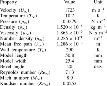
A similar procedure for the grid independence study was performed for the other two cases. As a result, for
 $H$
of 6.46 and 9.69, the standard grid corresponded, respectively, to a total of 33 800 and 41 600 cells, with a total of 710 400 and 896 300 molecules. A detailed discussion of the verification process, i.e. the effects of the cell size, time step and number of molecules on the aerodynamic surface quantities for the forward-facing step presented herein, is given by Leite (Reference Leite2009).
A.2. Validation process
The problem of a hypersonic rarefied flow over a flat plate is used to validate the two-dimensional version of the DSMC algorithm employed in this work. The exceptionally simple geometry makes it the most useful test case for the verification of the DSMC method through comparison with experiment. This model problem has been selected because both experimental data (Becker, Robben & Cattolica Reference Becker, Robben and Cattolica1974) and previous numerical simulations (Cercignani & Frezzotti Reference Cercignani, Frezzotti, Muntz, Weaver and Campbell1989; Hermina Reference Hermina1989; Hurlbut Reference Hurlbut1989; Lord Reference Lord, Shizgal and Weaver1994) are available for comparison. Therefore, a flat plate with the same characteristics as that investigated by Becker et al. (Reference Becker, Robben and Cattolica1974) was adopted in this work as the DSMC test case. Since these data have been published elsewhere, details will be kept to a minimum and the discussion will be restricted to the significant conclusions.
According to Becker et al. (Reference Becker, Robben and Cattolica1974), a flat plate of 50.8 mm in length, 25.4 mm in width and with a leading-edge thickness of 0.04 mm was positioned along the centreline of a helium jet gas. The helium flow field was generated by a free jet expansion from a distance from the flat plate that resulted in a free stream Mach number of 8.9, free stream temperature of 10.7 K and free stream pressure of
 $0.337~\text{N}~\text{m}^{-2}$
. The free stream Knudsen number, based on the plate length, was 0.0253. Table 9 summarizes the free stream and flow conditions for the DSMC test case.
In the computational solution, it was assumed that the flat plate was immersed in a uniform stream flowing parallel to the plate itself. The flat plate was modelled as one with zero thickness and a length of
 $80{\it\lambda}_{\infty }$
. The undisturbed free stream boundary conditions were imposed
 $5{\it\lambda}_{\infty }$
upstream of the plate leading edge, and the outer boundary was positioned at a distance of
 $30{\it\lambda}_{\infty }$
from the plate surface. The computational domain was divided into two regions, region 1 (
 $5{\it\lambda}_{\infty }\times 30{\it\lambda}_{\infty }$
) with
 $10\times 40$
cells and region 2 (
 $80{\it\lambda}_{\infty }\times 30{\it\lambda}_{\infty }$
) with a total of
 $300\times 80$
cells. The cell spacing was non-uniform in both directions. This grid was designated as the standard case, which corresponded to a total of 24 400 cells and approximated a total of 512 600 molecules. In addition to this high-resolution grid, two other grids, defined as coarse and fine, were used to study the sensitivity of the computations to grid resolution. Details of this grid independence study are given in Leite (Reference Leite2009).
Density ratio (
 ${\it\rho}/{\it\rho}_{\infty }$
) profiles normal to the flat-plate surface for three sections along the flat plate: (a)
 $x=0.5~\text{mm}$
, (b)
 $x=2.5~\text{mm}$
and (c)
 $x=6.5~\text{mm}$
. Solid lines represent the present DSMC simulations, full and empty symbols represent experimental and numerical data respectively.

Tangential velocity ratio (
 $u/U_{\infty }$
) profiles normal to the flat-plate surface for three sections along the flat plate: (a)
 $x=0.5~\text{mm}$
, (b)
 $x=2.5~\text{mm}$
and (c)
 $x=6.5~\text{mm}$
. Solid lines represent the present DSMC simulations, full and empty symbols represent experimental and numerical data, respectively.

Density profiles normal to the flat-plate surface are illustrated in figures 27(a–c) for three axial positions along the flat plate. In this set of diagrams, the density
 ${\it\rho}$
is normalized by the free stream density
 ${\it\rho}_{\infty }$
, and the dimensionless height
 $Y$
corresponds to the height
 $y$
above the flat-plate surface normalized by the free stream mean free path
 ${\it\lambda}_{\infty }$
. In addition, solid lines represent the present DSMC simulations, and full and empty symbols correspond, respectively, to experimental and numerical data available in the literature. The numerical simulation data shown were obtained by Cercignani & Frezzotti (Reference Cercignani, Frezzotti, Muntz, Weaver and Campbell1989) by means of the Boltzmann equation, and by Hermina (Reference Hermina1989), Hurlbut (Reference Hurlbut1989) and Lord (Reference Lord, Shizgal and Weaver1994) by employing the DSMC method. It is immediately evident from figures 27(a–c) that there is a close overall agreement between the present DSMC simulation and the measured and calculated data near the leading edge of the flat plate.
Temperature ratio (
 $T/T_{\infty }$
) profiles normal to the flat-plate surface for three sections along the flat plate: (a)
 $x=0.5~\text{mm}$
, (b)
 $x=2.5~\text{mm}$
and (c)
 $x=6.5~\text{mm}$
. Solid lines represent the present DSMC simulations, full and empty symbols represent experimental and numerical data respectively.

Tangential velocity profiles normal to the flat-plate surface are displayed in figures 28(a–c) for the same three axial positions. In this group of plots, the tangential velocity
 $u$
is normalized by the free stream velocity
 $U_{\infty }$
. The comparison of the computed results with experimental data shows that in the vicinity of the leading edge the computed velocities show good agreement with the measured velocities.
In an analogous fashion, variations in the temperature
 $T$
profiles, normalized by the free stream temperature
 $T_{\infty }$
, are displayed in figures 29(a–c). Once again, it is immediately evident that there is close overall agreement between the present DSMC calculations and the other computational results for temperature profiles.