INTRODUCTION
For a long time the prevailing view of exchange rate formation was that exchange rates were essentially determined by “fundamentals,” however the latter might be defined. Yet many of the stylized facts concerning the observed time series of exchange rates can be better explained by models that relax some of the assumptions of fundamentals-based models, which are closely related to the “efficient markets” hypothesis. This is true, in particular, for models that take explicit account of the way in which individuals form their expectations and the way in which that process is influenced by the other individuals in the market, and this will be the subject of this paper.
Considerable doubt has been cast on the theoretical consistency and the empirical validity of fundamentals-based models and in particular the efficient markets hypothesis. In financial markets in general the price of an asset is assumed to reflect the fundamentals, which are given by the discounted sum of the stream of earnings that that asset will yield over time. In foreign exchange markets, which are what will concern us here, this can be translated into saying that the fundamentals are reflected in the real interest differential between the countries that emit the various currencies. Yet it has long been observed that asset prices have higher volatility than the underlying fundamentals. This “excess volatility” puzzle has generated a large literature. There are those who argue that there is indeed excess volatility [see, e.g., Le Roy and Porter (1981), Shiller (1981), Blanchard and Watson (1982), and for a recent comprehensive analysis, Lo and MacKinlay (1999)]. The discussion has not been completely one-sided, however, and it was suggested, in reply to the first criticisms, that it may be the testing procedure that is at fault [for a discussion see Campbell and Shiller (1987) or West (1987) for example] and that prices do, in fact, contain all pertinent information. The overall result of the debate seems to have been that the underlying model is indeed flawed and the next step is to seek possible explanations and alternatives.
In the specific exchange rate context, the standard model, based on the fundamentals of the system, is the so-called real interest differential model, which was given its definitive expression by Hooper and Morton (1982). As in most of the models developed in the eighties and nineties, the fundamentals used are some subset of the money supply, real income, the expected inflation rate, the nominal rate of interest, and the current account balance. Models of this sort performed very poorly from a forecasting point of view, as indicated by Meese and Rogoff (1983, 1988) and Edison (1991). Doubts were cast on the existence of a consistent relation between exchange rates and fundamentals. With the improvement of econometric techniques, models were developed that took into account the nonstationarity of the exchange rate and fundamental time series. Cointegration models such as those used by Chinn and Meese (1995), Mark and Choi (1997), MacDonald and Marsh (1997), and Mark and Sul (2001) seem to establish a long-run equilibrium relation between exchange rate and fundamentals, as do the error correction models used by Campbell and Schiller (1987). Although these models have been challenged because of the fragility of the results [see Diebold ET AL. (1994) and Sephton and Larsen (1991)], even if accepted, they raise an important problem. Expectations play a key role in any exchange rate model, and if the relation between exchange rates and fundamentals is truly a long-term one how can agents who often have relatively short horizons be expected to use this relation to determine their forecasts?
A possible resolution of this difficulty may lie in the fact that the standard model says little about the way in which the market processes the information that is available into prices. One way of thinking of markets is to consider them as algorithms that transform information into prices. In the case that will concern us in this paper, the foreign exchange market, Lyons (2001) has taken this problem seriously and shows how information may be transformed into prices as a result of the order flows observed by traders or market makers. Thus, we can see how the information from those who give orders is transformed through the market into price signals. Such transmission may be far from perfect and, in particular, the different horizons of the individuals in the chain will be important.
What is it that generates the orders that, in turn, generate current prices? Individuals have preferences and forecasts as to future prices. This, coupled with their wealth, will generate their demand. What Lyons is suggesting is that the demands alone will not explain the evolution of prices, because these are intermediated by individuals who themselves take positions. This complicated process may lead to some of the features that one observes in actual markets. Lyons focuses on the process of equilibration, how the arrival of orders that then enter a dealer's order book will convey information to the dealer, and how that, in turn, will affect the prices quoted. However, Lyons's emphasis is on the idea that this complicated process of transmission will lead to efficient outcomes in the standard sense. Thus the presence of varying expectations will not perturb the market from its true course. Yet more attention has been paid to the idea that some individuals not only may not forecast on the basis of fundamentals, but also may have an important influence on the evolution of prices.
Such considerations gave rise to a series of models in which agents forecast purely on the basis of previous exchange rates, which are frequently referred to as “chartist” models. These models were contested by theorists on the grounds that, if fundamentals really do determine exchange rates in the long run, then arbitrageurs would take positions that would remove any profits that chartists might have made. Nevertheless a series of papers starting with DeLong ET AL. (1990) showed that chartists could, under quite reasonable assumptions, consistently make money, and this was confirmed by LeBaron (1999).
The empirical evidence is mixed, Curcio ET AL. (1997) arguing that chartist or technical rules are not profitable, whereas Dooley and Schafer (1983), Sweeney (1986), Levich and Thomas (1993), and Neely ET AL. (1997) suggest that technical rules can be shown to be profitable. More recently, Dewachter (2001) showed that Markov switching regime models could be profitable.
This raises a natural question. Do traders actually use technical rules? Allen and Taylor (1990) and Menkhoff (1997) conducted surveys in London and Frankfurt. The former found that 90% of traders used at least a chartist component in their short-term forecasts and that a majority of them found that the chartist component was at least as important as the fundamentals. In the long run, agents using methods based solely on fundamentals composed 30% of the total, whereas, on the other hand, 86% found that fundamentals were more important than extrapolations. Menkhoff's results are strikingly similar.
We are then faced with a paradox. There seems to be some evidence of a long-term relation between exchange rates and fundamentals, and agents acknowledge this, but in the short run they overwhelmingly use chartist methods and there is some evidence that these are indeed profitable. The only reasonable answer seems to be to use models in which fundamentalists and chartists coexist, as suggested by Frankel and Froot (1988) and Goodhart (1988).
In this paper we not only allow for the coexistence of chartists and fundamentalists but also allow for individuals switching between the two types of forecasts, as in Kirman (1993) and Kirman and Teyssiere (2002). Whereas in the latter model the supply of foreign currency from the foreign investors was exogenous, in the model presented here this supply is endogenous and results from the choices of fundamentalist or chartist foreign investors. As shown by Kirman and Teyssiere (2000), such models capture certain features of the real data, such as long memory. They also eliminate some of the contradictions inherent in the evidence by allowing traders to vary the importance they attach to fundamentals over time. The choice, made by the investors, either domestic or foreign, between the forecasting rules representing their beliefs about the functioning of the market, that is, fundamentalist or chartist, is probabilistic. To be more precise, it is made by a drawing from a Logit probability law that is exponential, and where the exponent is positively proportional to the discounted cumulative gain obtained from using the rule in question. Thus, the probability is an increasing function of the cumulative gain. Then, every investor revises his or her beliefs according to an exploration-exploitation process. Such a process emphasizes the forecasting strategy that has been the most profitable in the past—exploitation—but the choice of the other strategy is still possible—exploration. Finally, the investor demand for foreign currency is determined according to a standard model of the theory of finance [Grossman (1976)]. Thus we concentrate on the way in which individuals change their expectations and how this then changes their demands. We do not study the precise way in which markets equilibrate, but assume that prices adjust to clear the market in each period. Thus we analyze a series of temporary equilibria.
Unlike most models, in which the changing expectations of individuals cause movements in the exchange rate [see Goeree and Hommes (2000), Lux (1998)], we consider both sides of the market; that is, we think of a situation in which there are two countries and there are domestic and foreign traders who will take positions in each other's assets. This avoids some of the artificial features found in the single-country trading models and allows us to examine the coordination that may occur between the expectations in the two countries. In each country there are what are considered as domestic fundamentals by their inhabitants, and these may be strongly related. To be more explicit about the two types of expectation that may prevail in the tradition of Frankel and Froot (1990) and the literature based on their idea, we define them as follows. There is a “fundamentalist” point of view that takes the position that there is an equilibrium value of the exchange rate based on fundamentals and that the rate will tend towards that value. There is also a “chartist” point of view that simply forecasts on the basis of an extrapolation from previous values. We will give an explicit form to these extrapolations, but any rule that conditions only on past values of exchange rates will serve the purpose. There will be chartists and fundamentalists in each country and the proportions will depend on the success that individuals have had, in the past, from following the two forecasting rules.
Recall that a standard formulation of the exchange rate model can be written

where st is the current or spot exchange or its logarithm,
is the expected change in the exchange rate,
, conditioned on current information, It, and zt is a vector of fundamentals.1
The following notation is used throughout the paper: any stochastic variable is denoted with a tilde, e.g., any nonobserved variable such as the exchange rate of the next period
, whereas any realization of a variable is denoted by the same symbol without any particular sign, e.g., the observed exchange rate value of the current period st or the agent's information set It.
, which can be interpreted as the market forecast based on a weighted average of the two forecasting rules. The weights will depend on the relative number of traders using each rule and the market forecast will not necessarily be the same in the two countries. Furthermore, the market forecasts will evolve as the proportions of fundamentalists and chartists change over time.
Having developed our basic model, we will then analyze the effect of the evolving beliefs of the traders in the two countries on the exchange rate, and we will examine the uniqueness of the equilibrium and the dynamic evolution of the exchange rate. We will finally simulate the model in order to evaluate our theoretical conclusions and to get an idea as to the relative influence of the various parameters on the exchange rate time series.
THE MODEL
We assume the following:
There is one domestic exchange market on which are traded two currencies, domestic d and foreign f, whose values are linked by the exchange rate s. The variable s is the price of one unit of foreign currency in units of domestic currency, so that, from the point of view of a domestic investor, a devaluation of her currency means an increase in the value of s. For convenience, we define the exchange rate in terms of foreign currency as
.
There are n domestic and m foreign investors; the former measure their wealth in units of d and the latter in units of f (investors of one kind are all identical, i.e., they have the same risk aversion and the same utility functions).
Investors can hold one of two views as to the evolution of the exchange rate.
Consider the case of the domestic investor who wishes to forecast the value of the exchange rate of the next period, which is not observed when the expectation is determined,
(the case of the foreign investor is symmetric).
If the investor is a fundamentalist, he or she believes there is a fundamental value
that is observed before the expectations are determined and to which the equilibrium exchange rate will revert. We attribute the following form to these beliefs:

If the investor is a chartist, his or her forecast as to the future value of the exchange rate will be an extrapolation of its past values. We give these extrapolations the following form:

Now define the following variables at time t:
- ρ is the dividend in foreign currency paid on one unit of foreign currency;
- r is the interest rate on domestic assets;
- st is the exchange rate of the current period t;
- is the demand by individual i for foreign currency;
- is the demand by individual i for domestic currency.
The wealth of individual i at time t is determined by his or her investments in foreign and domestic assets and what he or she earned on them. That is,

At each point in time the individual's demands for foreign and domestic assets must satisfy the budget constraint

The discounted financial gain for individual i in period t is given by

where ω is the discount factor. Explicitly, it reads

Note that if ω=0, then the financial gain in the period is

which is the sum of the interests
paid on the investor i's portfolio
and the capital gain
. And the cumulative gain is given by

where
is the wealth of individual i at the beginning of period one (before she chooses the rule to be used).
However, the gains in each period are determined by the demands for domestic and foreign currency in the previous period, and these are, in turn, determined by the forecast that the individual made as to the exchange rate in the next period. The latter depends on whether he or she was following the fundamentalist or chartist rule. As already mentioned, the choice of rule is made by a drawing from a Logit probability law. It is a stochastic individual behavioral learning process. We want to keep a total of the gains obtained up to period t by following the fundamentalist rule and similarly for the chartist rule. Define a random variable
that will take on two values F and C; that is,

Now we can define an indicator function for the random variable, and this is simply

This leads to the gains for an individual using each forecasting rule as

where
is the investor i's financial gain at the current period, which is a function of his or her beliefs
and of the equilibrium exchange rate sr−1, as shown further in the paper, and with
.
An alternative model—not investigated in the paper—would be one in which everyone is able, ex post, to calculate what his or her gains would have been had he or she used the other rule. In this case all agents would attribute the same gains to each rule, that is,

where
and
denote the gain that would have been obtained by an individual using the rules F and C, respectively, in the period t−1. Of course, this depends on the fact that the individual's gains depend only on the forecasting rule chosen and not on his or her wealth, as will be the case for the class of utility functions that we will consider in this paper. Such a rule corresponds to a collective behavioral learning process.
The first piece of information that investor i is the rule
he or she has drawn. What is the remaining information
of a domestic investor i at time t? He or she has observations of the past values of his or her demands for foreign and domestic assets in the previous periods, the vector of observed exchange rates up to period t−1 and the cumulated gains that he or she has realized from using each of the two forecasting rules, fundamentalist and chartist. Thus we have

The total information available to the individual i once a forecasting rule has been determined is given by
. The total information of a foreign investor j has the same form, with the foreign currency replaced by the domestic and vice versa, and the exchange rate replaced by its inverse.
We now turn our attention to the derivation of the individual i's demand for foreign assets and, given his or her budget constraint, this will also determine his or her demand for domestic assets.
The Demand of a Domestic Investor for Foreign Currency
Consider the set of domestic investors D. Any i in D determines his or her optimal demand for risky currency according to the standard Grossman (1976) model, which states that the investor maximizes the expected utility of his or her wealth in the next period t+1. So the investor has the following problem:

where the investor's wealth in the next period, t+1, is given by

In this paper we choose, on the one hand, the very simple mean-variance utility function,

where μD is the measure of risk aversion. The expectations of the investor depend on whether he or she is following the fundamentalist or the chartist rule.
Hence, using first-order conditions, we can write the demand for agent i as

As for the CARA utility function, the optimal demand does not depend on the agent's wealth in the current period t.
Clearly the expectations in equations (12) and (15) are conditioned on which rule the agent is following, and recalling the definition of the indicator function for the random variable given in equation (7), we can write

Recall, finally, that the demand for the individual i when he or she is using the rule F or C is given by replacing the expectation in (13) by the expectations for each of the rules that were defined in (2) and (3):
(i) for the fundamentalist,

(ii) for the chartist,

The Demand for Domestic Assets by a Foreign Investor
The Demand for Domestic Assets by a Foreign Investor is obtained in a precisely analogous manner for each investor j in the set of foreign investors F. The wealth of an individual is now measured in foreign currency, for whom the risky investment is in domestic assets, the safe rate of interest is that in the foreign country, ρ, and the exchange rate
. Thus we can write the foreign investor's demand for domestic currency as

and, as in the case of the domestic investor, he or she will use one of the two rules given by (2) and (3), with st replaced by et. Thus we have

The Market Equilibrium
Consider first the aggregate demand for foreign currency of the domestic investors. This is given by

or, if we define the number of domestic investors who use the fundamental rule at time t as ND,t(F) and the total number of domestic investors as ND, and
, then we can rewrite aggregate demand as

Now define analogously for the foreign investors their total number NF and the number of them who are fundamentalists at time t by NF,t(F) and
. Then we can write the aggregate demand for domestic assets by foreigners as

The equilibrium exchange rate
is then determined by the equilibrium condition, given in the domestic currency, of the foreign exchange market,

where
(Γt) is the value in domestic currency of the demand for foreign (domestic) currency of the domestic (foreign) investors. It also reads

where

Having specified our model, we can now turn to the basic analytic results.
RESULTS
Analytical Results
The first result (Proposition 1) establishes the existence and uniqueness of the temporary equilibrium at each point in time and the second the properties of the probability that an investor chooses the fundamentalist rule (Proposition 2).
The equilibrium exchange rate
PROPOSITION 1. Let
be the exchange rate for which the second derivative with respect to the exchange rates of the excess demand is equal to zero and let
be the maximum of the first derivative. Let s1 and s2 be the values of the exchange rate such that the first derivative of the excess demand equals 0.
Define the following auxiliary variables:

The equilibrium exchange rate
exists, is positive, and is unique, unless the following conditions hold:

Proof. The equilibrium exchange rate is that for which the excess demand is equal to zero; it is the solution of the polynomial of degree 3 that is the equilibrium condition (23). The analysis of the variations of the excess demand according to the parameter values of the demand and the supply of foreign currency gives the conditions to be fulfilled for the equilibrium condition (23) to have either one real solution, that is, one equilibrium state, or three real solutions, that is, three equilibrium states (see Appendix).
Interpretation of Proposition 1. Condition (i) can be more easily interpreted in the particular case where the numbers of investors, the interest rates, and the conditional variances of the exchange rates for the two countries are equal. Then
is equal to the cube root of the ratio
of risk aversions and the quantity
is the difference between, on the one hand, the expected gain for the domestic investors with respect to s, and on the other hand, what can be considered as an “expected” gain for the foreign investors, defined as the difference between the inverse of the square of the expected exchange rate e=1/s and the inverse of the square of s.
In the particular case of interest, the proposition says that, if the domestic and foreign investors' expectations and risk aversion are such that
, then the exchange rate exists, is positive, and is unique.
The probability of choosing a rule.
As already mentioned, after the equilibrium exchange rate of the current period has been determined and consequently the investor knows his or her gain, each investor chooses the rule he or she is going to use to determine his or her demand for the next period. The probability of individual i being a fundamentalist at time t is given by

which can be rewritten as

where

defined as in (9), that is,

To analyze the properties of the probability of an investor choosing the fundamentalist rule, we can drop the i superscript in (25), because all individuals calculate the gains from each strategy in the same way. Then the evolution of the two groups, the fundamentalists and the chartists, in each country can be deduced. Clearly this will depend on the success of the two strategies. The extreme cases are defined by the extreme magnitudes of the ratio
between the coefficient of cumulative gain and the coefficient of risk aversion in the above probability. They are illustrated by the following result:
PROPOSITION 2 Investor i has the following extreme probability of choosing the fundamentalist rule:

Proof
This is easily obtained using equations (26), (9), and (7):

What this result says is that, if one rule gets the direction of the change of the exchange rate wrong, and the ratio of the importance the investor attaches to his or her previous experience, which is given by β, to his or her coefficient of risk aversion, μ, becomes large, then the probability of its being used will tend to zero. On the other hand, if the investor does not attach much importance to the past or is very risk-averse, the proportions of the two types will fluctuate around one-half.
An alternative.
So far, we have been considering the individual's probability of choosing a forecasting rule as dependent on his or her own strategy. We could, on the other hand, as already presented as an alternative, consider that he or she is capable of evaluating what he or she would have gained from adopting the alternative strategy, and in this case gains would be given by (9)

Analyzing the consequences of such a modification is the subject for future research.
Simulation Results
We proceeded to run a number of simulations in order to analyze the effects of varying the crucial parameters of the model. In the simulated model we introduced a discount factor ω for past gains, which is clearly related to the weight β that individuals attach to their previous experience. The higher the discount factor ω, the less likely the individual is to become locked into one of the forecasting rules, as is the case when β is low. Our basic purpose is to study the effect of modifying the following parameters of the time series:
The variable β is the weight attached to exploitation as opposed to exploration with respect to previous gains.
The variable μ is the coefficient of risk aversion.
In particular, we will consider the ratio
, which plays a special role in the model.
The variable ν is the rate at which individuals following the fundamentalist rule believe the exchange rate will return to its true value.
The variable ω is the rate at which individuals discount past gains.
The domestic and foreign interest rates, as well as the number of investors in each country, are kept constant. The fundamental exchange rate in each country is taken as exogenous and different.
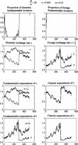
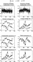
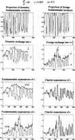
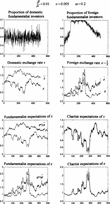
According to Proposition 1, when three real values are obtained as equilibria, a “continuity” argument is used to choose the real value that is closest to the previous unique solution. In the simulations that are shown to clarify the results (Figures 1–4), the parameter ν is the coefficient of the first-order adjustment term, which enters the definition of the fundamentalist expectations, equation (2); and when it takes a small value, ν=0.005, this means that the expectations are almost equal to the fundamental exchange rate.

Simulation 1.

Simulation 3.

Simulation 6.

Simulation 8.
The main results of the simulations, run using Matlab software over 500 periods of time, are the following:
(I) The dynamics of the proportions of domestic or foreign investors has the following characteristics:
(A) If β/μ[Gt ]1, the proportion changes rapidly from 1 to 0; the agents are almost all either “fundamentalists” or “chartists.” The value taken by the discount factor ω used in the calculation of the cumulative gain determines the qualitative aspect of the changes:
(1) If all the past gains have the same weight, 1−ω close to 1, then the number of changes of the proportion from 0 to 1, or vice versa, is small in number (1 to 3) and in this case the proportions remain a relatively long time at a given value (0 or 1); see simulation S1 in Figure 1.
(2) If only the recent past values of the gains are taken into account, 1−ω close to 0, then the number of changes of the proportion from 0 to 1, or vice versa, is very large in number and the proportion oscillates very rapidly between the values 0 or 1; see simulation S6 in Figure 3.
(A) If β/μ[Lt ]1, the proportions oscillate rapidly about the value one-half, and the agents are almost equally distributed among “fundamentalists” and “chartists.” The value of the discount factor determines the qualitative aspect of the changes, which in this case is not as clear-cut as in the previous case: whatever the value of the discount factor be, either close to 0 or to 1, the proportions oscillates very rapidly but the amplitude of the oscillations is small, in the sense that the values are taken in the interval between 0.35 and 0.65; see simulations S3 and S8 in Figures 2 and 4.
(II) The dynamics of the equilibrium exchange rate when the expectations are of the “fundamentalist” type and have values close to the fundamental shows the following characteristics:
(A) If β/μ[Gt ]1
(1) If 1−ω is close to 1; see simulation S1:
(a) If the proportion of domestic “fundamentalist” investors is close to 1 and the proportion of foreign “fundamentalists” is small, then the equilibrium exchange rate follows the domestic fundamental exchange rate and its inverse is very different from the foreign fundamental exchange rate.
(b) In the opposite case the exchange rate differs substantially from the national fundamentals and the inverse is very close to the foreign fundamentals.
(2) If 1−ω is close to 0, see simulation S6: the exchange rate exhibits higher volatility than when the discount factor 1−ω is close to 1.
(B) If β/μ[Lt ]1
(1) If 1−ω is close to 1, see simulation S3: the exchange rate never comes close to the fundamental, as was the case for β/μ[Gt ]1.
(2) If 1−ω is close to 0, see simulation S8: the exchange rate shows a behavior qualitatively equivalent to that obtained when the discount factor is close to 1.
(III) The comparison between Cases (2.A) and (2.B) shows the important role played, ceteris paribus, by the following:
(A) The ratio β/μ, which has an important influence on the dynamics of the proportions of fundamentalist investors as well as the dynamics of the exchange rate, which diverges from the fundamental when this ratio is relatively weak.
(B) The discount factor, which can induce fast fluctuations with large amplitude of the proportion of fundamentalist investors when it is close to 1 (1−ω close to 0); and furthermore, the volatility of the exchange rate is also increased.
CONCLUSIONS
The results that have been obtained here show that, as we suggested at the outset, a rather basic model in which traders of different national origins who trade in the same market using simple rules to form their expectations can generate complicated dynamics at the aggregate level. We should also emphasize the extreme sensitivity to certain important parameters of the dynamics of the proportions of domestic or foreign investors who chose the fundamentalist strategy to determine their expectations. This is also true of the equilibrium exchange rate, whose time path varies according to the values of the crucial parameters of the exploration/exploitation process used by the domestic or the foreign investors. The process that is used to revise the beliefs involves the following parameters: risk aversion μ, coefficient β of the cumulative gain which intervenes in the probability to draw the “fundamentalist” strategy, discount factor ω to calculate the cumulative gain, etc. Although the particular time path followed will depend on the specific values of the parameters, it is also worth noting that the general structural characteristic of the process do not depend on this choice. [The proof of this is given in Foellmer ET AL. (2005)].
Further developments will be to make the choice of the rule, fundamentalist or chartist, endogenous and/or to replace the individual behavioral learning process extensively presented in the paper with a collective behavioral learning process suggested as an alternative.
APPENDIX: TABLE OF VARIATIONS OF THE EXCESS DEMAND D – Γ