1. Introduction
The universe abounds with examples of turbulent flows that are driven by buoyancy and constrained by rotation. These highly complex flows shape our environment across scales: in protoplanetary disks, they mediate the formation of planetesimals (Lesur & Ogilvie Reference Lesur and Ogilvie2010); in planetary atmospheres, including on Earth, they carry heat, momentum and moisture, crucially impacting the climate (Emanuel Reference Emanuel1994; Dauxois et al. Reference Dauxois2021; Siegelman et al. Reference Siegelman2022); in the Earth’s oceans (Marshall & Schott Reference Marshall and Schott1999; Cheon & Gordon Reference Cheon and Gordon2019), they transport heat, carbon dioxide and nutrients, thereby crucially influencing biotopes (Severin et al. Reference Severin, Conan, Durrieu de Madron, Houpert, Oliver, Oriol, Caparros, Ghiglione and Pujo-Pay2014); in planetary and stellar cores, they are responsible for the generation of large-scale magnetic fields via the dynamo instability (King et al. Reference King, Soderlund, Christensen, Wicht and Aurnou2010; Jones Reference Jones2011; Schaeffer et al. Reference Schaeffer, Jault, Nataf and Fournier2017); in the subsurface oceans of the gaseous giants’ moons, they shape the icy crusts of Europa, Enceladus, Titan, etc. (Pappalardo et al. Reference Pappalardo1998; Mitri & Showman Reference Mitri and Showman2008; Nimmo & Pappalardo Reference Nimmo and Pappalardo2016; Soderlund et al. Reference Soderlund, Rovira-Navarro, Le Bars, Schmidt and Gerkema2024); in stars like the Sun (Miesch Reference Miesch2000; Fan Reference Fan2021) they are responsible for large-scale magnetic fields as well as rich dynamics such as the 22-year cycle in solar activity.
Such geo- and astrophysical flows, in spite of their differences, typically share two important properties. Owing to their turbulent nature, their dynamics results from a broad range of interacting spatial and temporal scales. Accordingly, advection by the flow dominates over viscous forces when the Reynolds number is large,
 ${Re}_H=UH/\nu \gg 1$
, based here on the fluid layer depth
 $H$
, a typical velocity of the flow
 $U$
and kinematic viscosity
 $\nu$
. Simultaneously, advection by the flow occurs on time scales much longer than the planetary rotation period, as measured by small Rossby numbers
 ${Ro}_H=U/(2\Omega H)\ll 1$
, where
 $\Omega$
is the planetary rotation rate.
Also of particular importance is the ratio of the viscous and Coriolis forces providing an a priori external parameter referred to as the Ekman number
 ${Ek} = {Ro}_H/{Re}_H = \nu /(2\Omega H^2)$
, as well as the Prandtl number
 $\sigma = \nu /\kappa$
characterising the fluid under consideration, where
 $\kappa$
is the thermal diffusivity. The strength of the thermal forcing is controlled by the Rayleigh number
 ${Ra}$
, which is proportional to the temperature drop
 $\Delta _T$
across the fluid layer. This number can be used to define an alternate a priori parameter, the convective Rossby number
 ${Ro}_{{conv}}= \sqrt { {Ra}/\sigma }\, {Ek}$
, measuring the strength of the rotation relative to thermal forcing.
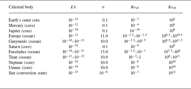
Celestial bodies typically feature extreme values for the non-dimensional parameters defined above, as summarised in table 1: rapid planetary rotation is reflected in very low Ekman and Rossby numbers, whereas large Reynolds numbers indicate the highly turbulent character of the flow. Such rapidly rotating, highly turbulent flows are challenging to analyse and specifically to simulate numerically owing to the sheer number of spatial and temporal degrees of freedom which they involve. One common approach for obtaining theoretical predictions at geophysically relevant parameters (specifically,
 ${Ek} \rightarrow 0)$
relies upon identifying transitions between different flow regimes in a region of more moderate parameters (
 ${Ek} \gtrsim 10^{-8}$
) that is amenable to direct numerical simulations (DNS) or laboratory experiments, together with the scaling laws for transport coefficients valid within each regime. These results are then extrapolated to extreme parameters on the assumption that the regimes and scaling laws observed for accessible parameter values extend to geo-/astrophysically relevant parameter values. Assuming that no non-trivial transition occurs outside the observed moderate parameter interval is a particularly strong assumption, akin to a leap of faith due to the current paucity of data at the most extreme parameter values.
Non-dimensional parameter estimates for planetary (Schubert & Soderlund Reference Schubert and Soderlund2011), satellite (Soderlund Reference Soderlund2019) and stellar interiors (Miesch Reference Miesch2000; Garaud & Garaud Reference Garaud and Garaud2008). Estimates of the Rossby number are derived from the relation
 $ {Ro}_{ {H}}= {Re}_{ {H}} {Ek}$
.

The dynamics of the fluid flows found in the celestial bodies listed in table 1 is further rendered complex by additional ingredients such as spherical geometry, multiple contributors to the density, compressibility and the presence of magnetic fields. Absent such complexities, the quintessential paradigm for investigating rotationally influenced buoyant flows is provided by rapidly rotating Rayleigh–Bénard convection (RRRBC). A large number of studies have been published on this model system, which is very well suited for detailed experimental, numerical and theoretical studies, see for example Chandrasekhar (Reference Chandrasekhar1953), Nakagawa & Frenzen (Reference Nakagawa and Frenzen1955), Veronis (Reference Veronis1959), Rossby (Reference Rossby1969), Boubnov & Golitsyn (Reference Boubnov and Golitsyn1986), Zhong et al. (Reference Zhong, Ecke and Steinberg1991), Julien et al. (Reference Julien, Legg, McWilliams and Werne1996), Knobloch (Reference Knobloch1998), Hart et al. (Reference Hart, Kittelman and Ohlsen2002), Vorobieff & Ecke (Reference Vorobieff and Ecke2002), Boubnov & Golitsyn (Reference Boubnov and Golitsyn2012), King et al. (Reference King, Stellmach and Aurnou2012), Stevens et al. (Reference Stevens, Clercx and Lohse2013) and the recent review by Ecke & Shishkina (Reference Ecke and Shishkina2023). In RRRBC, gravity is often taken to be antiparallel to the rotation axis on the assumption that the Froude number
 ${Fr}_\Omega \equiv \Omega ^2 H/g$
, where
 $g$
is the gravitational acceleration, is small. The resulting configuration is translation-invariant and believed to be relevant to the polar regions of planets, moons and stars as well as to their interiors, although the case of misaligned gravity and rotation axis has also been studied (Hathaway & Somerville Reference Hathaway and Somerville1983; Julien & Knobloch Reference Julien and Knobloch1998; Julien et al. Reference Julien, Knobloch, Milliff and Werne2006; Miquel et al. Reference Miquel, Xie, Featherstone, Julien and Knobloch2018; Novi et al. Reference Novi, von Hardenberg, Hughes, Provenzale and Spiegel2019; Cai Reference Cai2020; Currie et al. Reference Currie, Barker, Lithwick and Browning2020; Julien et al. Reference Julien, Ellison, Miquel, Calkins and Knobloch2025).
A major obstacle in the study of rapidly rotating convection, even in the highly idealised setting of RRRBC, is the difficulty, to date, of attaining the extremely low Ekman numbers, typically
 $10^{-12}$
or smaller (cf. table 1), that characterise geo- and astrophysical flows. By contrast, current state-of-the-art DNS of the full Navier–Stokes–Boussinesq equations that describe RRRBC have been restricted to
 ${Ek} \gtrsim 10^{-8}$
(Kunnen et al. Reference Kunnen, Ostilla-Mónico, van der Poel, Verzicco and Lohse2016; Guervilly et al. Reference Guervilly, Cardin and Schaeffer2019; Song et al. Reference Song, Shishkina and Zhu2024a
,
Reference Song, Shishkina and Zhub
), despite enormous computational effort. Inclusion of magnetic fields in the simulations to capture the capability for dynamo action, as well as spherical shell geometry, further limits the reported range of nearly all studies to
 ${Ek}\gtrsim 10^{-7}$
,
 ${Re}_H\lesssim 10^3$
(Schaeffer et al. Reference Schaeffer, Jault, Nataf and Fournier2017; Cooper et al. Reference Cooper, Bushby and Guervilly2020; Mason et al. Reference Mason, Guervilly and Sarson2022; Kolhey et al. Reference Kolhey, Stellmach and Heyner2022; Gastine & Aurnou Reference Gastine and Aurnou2023; Majumder et al. Reference Majumder, Sreenivasan and Maurya2024); simulations down to
 ${Ek}=10^{-10}$
are available for linearised dynamics only (He et al. Reference He, Favier, Rieutord and Le Dizès2022). State-of-the-art laboratory experiments are likewise restricted to
 ${Ek}\gtrsim 10^{-8}$
(Shew & Lathrop Reference Shew and Lathrop2005; Aurnou et al. Reference Aurnou, Calkins, Cheng, Julien, King, Nieves, Soderlund and Stellmach2015; Rajaei et al. Reference Rajaei, Kunnen and Clercx2017; Cheng et al. Reference Cheng, Madonia, Aguirre Guzmán and Kunnen2020; Lu et al. Reference Lu, Ding, Shi, Xia and Zhong2021; Hawkins et al. Reference Hawkins, Cheng, Abbate, Pilegard, Stellmach, Julien and Aurnou2023; Pothérat & Horn Reference Pothérat and Horn2024) although the Eindhoven TROCONVEX experiment is, in principle, capable of achieving yet lower
 ${Ek}\sim 5\times 10^{-9}$
, cf. Cheng et al. (Reference Cheng, Aurnou, Julien and Kunnen2018). These accessible parameter values in numerical or laboratory experiments are orders of magnitude larger than the estimates for realistic geo- and astrophysical applications. On the other hand, existing reduced equations (Julien et al. Reference Julien, Knobloch and Werne1998; Sprague et al. Reference Sprague, Julien, Knobloch and Werne2006), known as the non-hydrostatic quasi-geostrophic (NHQG) equations, describe the dynamics in the limit
 ${Ek}\to 0$
, but their applicability is, by construction, confined to asymptotically small values of
 ${Ek}$
. This leaves an unexplored gap corresponding to small but finite Ekman numbers, precisely the regime that is most relevant for geo- and astrophysical applications.
It is extremely rare to have a numerical or laboratory approach that allows one to span the parameter range from prototypical laboratory and DNS settings all the way to realistic geophysical and astrophysical settings. Remarkably, taking advantage of the characteristics of rapidly rotating thermal convection leads to a new numerical approach that relies on appropriately rescaled equations, and enables exploration of this very wide parameter range.
In the following section we describe the rescaled rapidly rotating Navier–Stokes equations (RRRiNSE) and sketch the numerical method used to solve them, followed in § 3 by a description of the results obtained, focusing both on bulk transport properties and the structure of the boundary layers at the top and bottom. The paper concludes in § 4 with a discussion of the significance of the RRRiNSE reformulation and prospects for future work. An Appendix provides additional details on the flow statistics and structure.
2. Methodology
In this section, we succinctly present the RRRiNSE, an equivalent reformulation of the full Navier–Stokes–Boussinesq equations, informed by the scaling behaviour valid in the limit of vanishing
 ${Ek}$
(Julien et al. Reference Julien, Knobloch and Werne1998; Julien et al. Reference Julien, Rubio, Grooms and Knobloch2012b
). The RRRiNSE formulation is described in detail in a recent paper (Julien et al. Reference Julien, van Kan, Miquel, Knobloch and Vasil2024), where it was first introduced and validated against existing results in the literature, and where the full details of the numerical implementation are given.
In short, the RRRiNSE retain all terms in the Navier–Stokes–Boussinesq equations while rescaling each variable according to its leading-order asymptotic scaling behaviour valid for
 ${Ek} \to 0$
in terms of the natural small parameter of rapidly rotating convection
 $\varepsilon \equiv {Ek}^{1/3}$
(Chandrasekhar Reference Chandrasekhar1953; Sprague et al. Reference Sprague, Julien, Knobloch and Werne2006). In particular, the rapid rotation generates a high degree of anisotropy, which is explicitly incorporated in the RRRiNSE formulation: vertical length scales are non-dimensionalised by the layer height
 $H$
, while horizontal length scales are significantly smaller, given by
 $\varepsilon H$
. Consequently, time is measured in units of the viscous diffusion time based upon
 $\varepsilon H$
. As shown by Julien et al. (Reference Julien, van Kan, Miquel, Knobloch and Vasil2024), this procedure ensures an adequate preconditioning of the equations of motion at small but finite
 ${Ek}$
, thus facilitating DNS in this highly relevant but unexplored regime.
2.1. Rescaled Navier–Stokes equations
The convective fluid layer confined by horizontal surfaces separated by a distance
 $H$
is subjected to rotation around the vertical axis
 $\boldsymbol {\Omega }=\Omega \boldsymbol {\widehat {e}}_z$
and uniform gravity
 $-g \boldsymbol {\widehat {e}}_z$
. The temperature difference between the bottom and the top plate is
 $\Delta _T\gt 0$
. In the Oberbeck–Boussinesq limit, the fluid density varies linearly with temperature
 $\rho = \rho _0 [1-\alpha (T-T_0)]$
near a reference state
 $(\rho _0, T_0)$
, with both the thermal expansion coefficient
 $\alpha$
, the fluid kinematic viscosity
 $\nu$
, and the temperature diffusivity
 $\kappa$
considered constant. The dimensional governing equations for the solenoidal velocity field
 $\boldsymbol {U}$
, the temperature
 $T$
and the pressure
 $P$
are
 \begin{gather} \partial _t \boldsymbol {U} + \boldsymbol {U\cdot \nabla U} + 2 \boldsymbol {\Omega } \times \boldsymbol {U}= -{{\frac {1}{\rho _0}}}\nabla P + \alpha g T \boldsymbol {\widehat {e}}_z + \nu \Delta \boldsymbol {U},\qquad \boldsymbol {\nabla \cdot U} = 0, \end{gather}
 \begin{gather} \partial _t T + \boldsymbol {U\cdot \nabla } T = \kappa \Delta T. \end{gather}
As described in detail by Julien et al. (Reference Julien, van Kan, Miquel, Knobloch and Vasil2024), the power behind the RRRiNSE formulation lies in their use of rotation-influenced characteristic scales for non-dimensionalisation. For convenience, we introduce the small parameter
 $\varepsilon \equiv {Ek} ^{1/3} = (\nu /2 \Omega H^2 )^{1/3}$
and measure lengths in units of the layer depth
 $H$
in the vertical, but in units of
 $\ell _*=\varepsilon H$
in the horizontal, so that
 $(X,Y,Z)=(\varepsilon H \widetilde {x}, \varepsilon H \widetilde {y},H\widetilde {z})$
. In these coordinates, the rescaled anisotropic gradient
 $\boldsymbol {\nabla }=\varepsilon ^{-1}H^{-1}\boldsymbol {\widetilde {\nabla }}_\varepsilon \equiv \varepsilon ^{-1}H^{-1}(\partial _{\tilde {x}}, \partial _{\tilde {y}}, \varepsilon \partial _{\tilde {z}})$
and the Laplace operator becomes
 $\Delta = \varepsilon ^{-2}H^{-2} \widetilde {\nabla }_\varepsilon ^2$
, where we have introduced the anisotropic diffusion operator
 $\widetilde {\nabla }_\varepsilon ^2 = \partial _{\tilde {x}\tilde {x}} + \partial _{\tilde {y}\tilde {y}}+ \varepsilon ^2 \partial _{\tilde {z}\tilde {z}}$
. All tildes will be dropped in the following. Time is non-dimensionalised using a diffusive time scale based on the horizontal scale rather than the layer depth alone:
 $t_*=\ell _*^2/\nu = \varepsilon ^2 H^2/\nu$
. Accordingly, the velocity scale is
 $U_*=\ell _*/t_*= \nu / (\varepsilon H)$
, giving the non-dimensional velocity
 $\boldsymbol {u} = \boldsymbol {U}/U_*\equiv (u,v,w)$
; the pressure scale
 $P_*=\rho _0 U_*^2/\varepsilon =\rho _0 \nu ^2/(\varepsilon \ell _*^2)$
is used to define the non-dimensional pressure
 $p\equiv P/P_*$
. This isotropic velocity scale, combined with our anisotropic coordinate system, results in horizontally dominated material derivatives
 \begin{equation} D_{t}^{\perp ,\varepsilon } = \partial _t + u \partial _x + v \partial _y + \varepsilon w\partial _z = \partial _t + \boldsymbol {u_\perp \cdot \nabla _\perp } + \varepsilon w \partial _z. \end{equation}
Here, the perpendicular symbol
 $\perp$
in the subscript denotes the projection upon the horizontal plane: specifically,
 $\boldsymbol {\nabla }_\perp = (\partial _x, \partial _y,0 )^\top$
and
 $\boldsymbol {u_\perp } = \boldsymbol {u} - w\, \boldsymbol {\widehat {e}}_z$
. The incompressibility condition becomes
 \begin{equation} \boldsymbol { \nabla _\perp \cdot u_\perp } + \varepsilon \partial _z w = 0. \end{equation}
The (dimensional) temperature
 $T$
is decomposed as the sum of three terms: an unstable linear stratification, a vertical profile
 $\Theta (z)$
, and horizontal fluctuations
 $\theta (x,y,z)$
with zero horizontal mean
 \begin{equation} T -T_0 = \Delta _T \left [1 - z + \Theta (z) + \varepsilon \theta (x,y,z) \right ], \end{equation}
where
 $0\leqslant z \leqslant 1$
. We thus formally embed in our decomposition one hallmark of rapidly rotating convection: horizontal temperature fluctuations are dominated by vertical variations. With these elements, the dimensionless governing equations for the horizontal fluctuations
 $(\partial _x, \partial _y) \neq (0,0)$
of momentum and temperature are found to be
 \begin{align} D_t^{\perp ,\varepsilon } \boldsymbol {u} + \varepsilon ^{-1} \boldsymbol {\widehat {e}}_z \times \boldsymbol {u}= -\varepsilon ^{-1}\boldsymbol {\nabla }_\varepsilon p + \frac { \widetilde {Ra}}{\sigma } \theta \, \boldsymbol {\widehat {e}}_z + {\nabla }_\varepsilon ^2\boldsymbol {u},\end{align}
 \begin{align} D_t^{\perp , \varepsilon } \theta + w \left (\partial _z \Theta -1 \right ) = \frac {1}{\sigma } {\nabla }_\varepsilon ^2 \theta ,\end{align}
where
 $ \widetilde { {Ra}}={Ek}^{4/3} {Ra}$
, and the Rayleigh number
 ${Ra}$
is given by
 ${Ra}= \alpha g H^3 \Delta _T /(\nu \kappa )$
in terms of the thermal expansion coefficient
 $\alpha$
of the fluid and gravitational acceleration
 $g$
. By denoting the horizontal average of any quantity using an overline
 \begin{equation} \overline {q}^{xy} \equiv \frac {1}{L_xL_y}\int _0^{L_x}\textrm {d}x\int _0^{L_y}\textrm {d}y\, q(x,y,z,t)\, , \end{equation}
we write separately the equations governing the vertical profiles of horizontal velocity
 $(\overline {u}^{xy}, \overline {v}^{xy})$
and temperature
 $\Theta$
 \begin{align} \partial _t \overline {u}^{xy} + \varepsilon \partial _z \overline {wu}^{xy} - \varepsilon ^{-1}\overline {v}^{xy} & = \varepsilon ^{2} \partial _{zz}\overline {u}^{xy} ,\end{align}
 \begin{align} \partial _t \overline {v}^{xy} + \varepsilon \partial _z \overline {wv}^{xy} + \varepsilon ^{-1}\overline {u}^{xy} & = \varepsilon ^{2} \partial _{zz}\overline {v}^{xy}, \end{align}
 \begin{align} \varepsilon ^{-2} \partial _t \Theta + \overline { \partial _z w\theta }^{xy} & = \frac {1}{\sigma } \partial _{zz}\Theta . \end{align}
Equations (2.4), (2.6) and (2.8) form the RRRiNSE system, which is analytically equivalent to the dimensional equations (2.1), (2.2) as we have only rescaled, but not discarded any terms in the equations. Numerically, however, these equations differ drastically in the sense that (2.4), (2.6) and (2.8) can be solved accurately for very small values of Ekmannumber, whereas the poor conditioning of the unscaled equations (2.1), (2.2) renders their solution impossible in practice whenever
 ${Ek}\lesssim 10^{-9}$
for reasons explained by Julien et al. (Reference Julien, van Kan, Miquel, Knobloch and Vasil2024).
2.2. Asymptotically reduced non-hydrostatic quasi-geostrophic equations
In the limit of rapid rotation
 ${Ek},{Ro} \to 0$
, one can derive a reduced set of governing equations for the flow (presented below) in a systematic and controlled way using asymptotic methods (Julien et al. Reference Julien, Knobloch and Werne1998; Sprague et al. Reference Sprague, Julien, Knobloch and Werne2006; Julien & Knobloch Reference Julien and Knobloch2007; Julien et al. Reference Julien, Rubio, Grooms and Knobloch2012b
). Here, we emphasise, in a quick sketch, how the rescaled equations (2.6) naturally lead to the reduced equations when the formal limit
 $\varepsilon \to 0$
is considered. Upon inspection, if the scaling employed for deriving the rescaled equations holds and all dimensionless variables remain
 $O(1)$
, the leading-order terms at order
 $O(\varepsilon ^{-1})$
in (2.6a
) indicate geostrophic balance
 \begin{equation} \boldsymbol {\widehat {e}}_z \times \boldsymbol {u}_\perp = -\boldsymbol {\nabla }_\perp p ,\end{equation}
so that the pressure serves as the geostrophic streamfunction
 \begin{align} \boldsymbol {u} &= - \boldsymbol {\nabla }\times (p\, \boldsymbol {\widehat {e}}_z ) + w\, \boldsymbol {\widehat {e}}_z + O(\varepsilon ) \end{align}
 \begin{align} &= -\partial _y p\, \boldsymbol {\widehat {e}}_x + \partial _x p \, \boldsymbol {\widehat {e}}_y + w\, \boldsymbol {\widehat {e}}_z + O(\varepsilon ). \end{align}
To obtain prognostic equations for
 $p$
,
 $w$
,
 $\theta$
,
 $\Theta$
we substitute expression (2.10) into the rescaled momentum equation and project the result upon
 $\boldsymbol {\widehat {e}}_z$
, obtaining at leading order in
 $\varepsilon$
 \begin{equation} \partial _t w + J[p,w]+ \partial _z p = \frac { \widetilde {Ra}}{\sigma }\theta + \nabla _\perp ^2 w, \end{equation}
where the Jacobian
 $J[p,w]\equiv \partial _x p \partial _y w - \partial _y p \partial _x w$
indicates horizontal advection of
 $w$
and
 $\nabla _\perp ^2\equiv \partial _{xx} + \partial _{yy}$
emphasises that horizontal diffusion dominates. We complement the vertical velocity equation with a governing equation for the streamfunction
 $p$
obtained by projecting the curl of the momentum equation on the vertical. Using incompressibility, one proves
 $\boldsymbol {\widehat {e}}_z \boldsymbol {\cdot \nabla }\times (\boldsymbol {\widehat {e}}_z \times \boldsymbol {u} ) = -\varepsilon \partial _z w$
, so that the leading-order contribution of
 $\boldsymbol {\widehat {e}}_z \boldsymbol {\cdot \nabla }\times$
(2.6a
) yields
 \begin{equation} \partial _t \nabla _\perp ^2 p + J[p,\nabla _\perp ^2 p] - \partial _z w = \nabla _\perp ^4 p. \end{equation}
Finally, one readily obtains the leading-order contribution to the governing equation for the temperature fluctuation
 $\theta$
and the mean temperature
 $\Theta$
 \begin{align} \partial _t \theta +J[p,\theta ] + w \left (\partial _z \Theta -1 \right ) &= \frac {1}{\sigma } {\nabla }_\perp ^2 \theta ,\end{align}
 \begin{align} \varepsilon ^{-2} \partial _t \Theta + \overline { \partial _z w\theta }^{xy} & = \frac {1}{\sigma } \partial _{zz}\Theta . \end{align}
Equations (2.11) constitute the reduced NHQG equations previously derived using a multiple-scale asymptotic expansion (Julien et al. Reference Julien and Knobloch1998; Sprague et al. Reference Sprague, Julien, Knobloch and Werne2006). These equations filter out fast inertial waves and thin Ekman layers and govern the leading-order geostrophically balanced flow.
The Ekman number dependence that remains in the governing equation (2.11d) for the mean temperature reflects the fact that the time scale
 $\tau = \varepsilon ^{2}t$
associated with the evolution of
 $\Theta$
is much slower than the convective time scale. Previous studies (Sprague et al. Reference Sprague, Julien, Knobloch and Werne2006; Julien et al. 2012b) have established that, in the limit of horizontally extended domains where a large number of convective cells or plumes contribute to the horizontal spatial averaging, this term can be omitted for the computation of global diagnostics of a statistically stationary state
 $\partial _t {\Theta }\approx 0$
. This assumption can be justified based on the following rationale: as the horizontal extent
 $L_\perp =L_x=L_y$
of the domain increases, so does the number of independent plumes
 $N_p$
that feed back into the temperature profile. The central limit theorem then suggests that, in the ergodic limit (time and ensemble averages behave similarly), the amplitude of temporal fluctuations of the vertical temperature profile
 $\Theta (z)$
should decrease like
 $1/\sqrt {N_p}\approx 1/L_\perp$
, justifying the neglect of the term
 $\partial _t\Theta$
. In the context of the RRRiNSE formulation, this assumption has been successfully validated and has proved to shorten the transient that leads to the stationary state (Julien et al. Reference Julien, van Kan, Miquel, Knobloch and Vasil2024). Thus in all simulations of the RRRiNSE (2.4), (2.6) and (2.8) and the NHQG equations (2.11) described in this paper,
 $\partial _t\Theta$
is set to zero, as is expected to be the case for a sufficiently large horizontal extent
 $L_\perp$
of the domain.
2.3. Details on the numerical method
We compute solutions to both the rescaled equations (2.4), (2.6) and (2.8) and the reduced equations (2.11) using the pseudo-spectral code Coral (Miquel Reference Miquel2021), a flexible platform for solving partial differential equations in a Cartesian domain. We assume periodicity in
 $(x,y)$
and thus decompose the problem variables using a Fourier basis in the horizontal, whereas a Chebyshev expansion is used in the vertical in order to impose boundary conditions on the bounding surfaces
 $z=0,1$
using a Galerkin basis recombination. Differential operators are discretised using the quasi-inverse method (Clenshaw Reference Clenshaw1957; Greengard Reference Greengard1991; Julien & Watson Reference Julien and Watson2009) to optimise memory usage and accuracy. The resolution was varied from
 $192$
grid points in each direction (corresponding to
 $128$
alias-free modes) at the lowest values of
 $\widetilde { {Ra}}$
, up to
 $768$
grid points (
 $512$
Chebyshev modes) in the vertical direction and
 $576$
grid points (
 $384$
Fourier modes) in the horizontal directions at larger
 $\widetilde { {Ra}}$
. The time marching relies on the family of stable semi-implicit Runge–Kutta schemes introduced by Ascher et al. (Reference Ascher, Ruuth and Spiteri1997), specifically their four-stage, third-order scheme, known as ARS443.
For some of the runs presented here, we have used low-amplitude noise as the initial condition, and waited for the convective turbulent flow to settle into a statistically stationary state after a transient period. However, for strongly supercritical flow, this transient may prove much more turbulent than the stationary state itself. Hence, in some cases, we resort to an alternative: instead of low-amplitude noise, the initial condition for a given run was taken from the solution computed at a neighbouring position in parameter space. This procedure facilitates the computation of the transient.
Once the transient has subsided, we compute time averages of different diagnostic quantities reported here. For instance, the barotropic vertical vorticity displayed in figure 2 is defined as
 \begin{equation} \overline {\omega _z}(x,y) = \int _0^1\omega _z\,\textrm {d}z, \end{equation}
where the vertical vorticity is given by
 $\omega _z=\partial _x v-\partial _y u$
. The Nusselt number is computed in terms of a volume average as
 ${Nu}(t) -1 = \sigma \langle w \theta \rangle _{{vol}}$
, where the volume average is given by
 \begin{equation} \langle \cdot \rangle _{{vol}} = \overline {\overline {(\cdot )}^{xy}} = \frac {1}{L_xL_y}\int _0^{L_x}\textrm {d}x\int _0^{L_y}\textrm {d}y\int _0^1 (\cdot )\textrm {d}z ,\end{equation}
and the small-scale Reynolds number based on the vertical velocity and the horizontal length scale is given, in the non-dimensional RRRiNSE formulation, by
 ${Re}(t) \equiv \sqrt {\langle w^2 \rangle _{{vol}}}$
. In addition, we denote the combined space and time average by
 \begin{equation} \langle \cdot \rangle = \frac {1}{t_2-t_1} \int _{t_1}^{t_2}\textrm {d}t \frac {1}{L_xL_y}\int _0^{L_x}\textrm {d}x\int _0^{L_y}\textrm {d}y\int _0^1 (\cdot )\textrm {d}z . \end{equation}
Overview of the parameter space. Panel a: estimates of the non-dimensional parameters for different celestial objects (see table 1) shown in the plane spanned by the Ekman and Reynolds numbers. The parameters reached in previous laboratory experiments and simulations are indicated by shaded regions. The dashed lines indicate regime boundaries discussed in the text: the green dashed line corresponds to the bulk Rossby number
 ${Ro}_H=1$
while the red dashed line corresponds to the local Rossby number
 ${Ro}_{ {BL}}=1$
in the thermal boundary layers (BLs). These lines are given by
 ${Re}_H = 1/{Ek}$
and
 $ {Re}_H={Ek}^{-3/5}$
, respectively. The regime bounded by these two dashed lines is characterised by unbalanced boundary layers and a balanced bulk flow. The symbols refer to the simulations summarised in panel b:
 $\widetilde { {Ra}}=const.$
(white diamonds),
 ${Ra}=const.$
(black triangles) and
 ${Ek}=const.$
(blue plus signs). Panel b: overview of simulations (with symbols identical to panel a) in the plane spanned by the reduced Rayleigh number
 $\widetilde { {Ra}}=Ra \, { {Ek}}^{4/3}$
and the Taylor number
 ${ {Ta}}={ {Ek}}^{-2}$
. Dashed lines represent regime boundaries corresponding to those in panel a.

3. Results
Here, we present the first DNS of RRRBC at realistically small Ekman numbers for planetary, satellite and stellar interiors, using the RRRiNSE formulation, and analyse the physics of the flow in this extreme parameter range. Our extensive set of simulations was performed using the pseudospectral solver Coral (Miquel Reference Miquel2021) for a periodic domain of horizontal extent
 $10\ell _c$
, where
 $\ell _c\approx 4.82{Ek}^{1/3}$
is the critical wavelength in the limit
 ${Ek} \to 0$
(Chandrasekhar Reference Chandrasekhar1953). Specifically, we consider a fluid with
 $\sigma =1$
subject to stress-free boundaries (for simplicity) at top and bottom where constant temperatures are imposed, and periodic boundary conditions in the horizontal directions. We explore unprecedentedly small but finite Ekman numbers, as low as
 ${Ek}=10^{-15}$
, values that are more than six orders of magnitude smaller than those previously attainable in DNS or in the laboratory.
3.1. Overview of parameter space
Figure 1(a) shows the parameter space explored in our simulations. The top panel shows the estimates of these parameters for planetary interiors and oceans on icy satellites given in table 1 in the plane spanned by the Ekman number
 ${Ek}$
and the bulk Reynolds number
 ${Re}_H$
, together with blue circles showing the values reached in our simulations, indicating that we attain realistically small
 ${Ek}$
equal to the estimated values for the outer core of the Earth (
 ${Ek}\approx 10^{-15}$
) and the convective zone of the Sun (not shown, cf. table 1). We further indicate the approximate range of parameters reached in previous numerical and laboratory studies, which are restricted to higher
 ${Ek}$
. Dashed lines highlight important regime boundaries where the Rossby number
 ${Ro}$
equals unity in different parts of the flow. The green dashed line is an estimate of where the bulk of the flow is expected to become rotationally supported as the rotation rate increases, namely
 ${Ro}_H=1$
, i.e.
 ${Re}_H = 1/{Ek}$
. In contrast, the rotation rate required to generate rotational support in the thermal boundary layers at the top and bottom is much higher. This rotation rate is determined by the condition that the local Rossby number in the thermal boundary layer
 ${ {Ro}}_{ {BL}}=1$
(red dashed line). As shown by Julien et al. (Reference Julien, Knobloch, Rubio and Vasil2012a
) this condition is satisfied when the convective Rossby number associated with the bulk flow
 ${ {Ro}}_{ {conv}}={ {Ek}}^{1/5}$
. With velocity following the rotational free-fall scale,
 $U=\alpha g \Delta _T H^2/(2\Omega )$
, we see that
 ${Re}_H={Ro}_{{conv}}^2/{Ek}$
, cf. Julien et al. (Reference Julien, van Kan, Miquel, Knobloch and Vasil2024), and hence that
 ${Re}_H={Ek}^{-3/5}$
(red dashed line in figure 1
a).
In rapidly rotating flows, higher values of
 $ {Ra}$
are required to trigger convection as a consequence of the Taylor–Proudman constraint (Proudman Reference Proudman1916). Specifically, the critical Rayleigh number for convection in the limit of small
 ${Ek}$
is proportional to
 ${Ek}^{-4/3}$
as shown by Chandrasekhar (Reference Chandrasekhar1953). Therefore, it is natural to introduce
 $\widetilde { {Ra}}\equiv RaEk^{4/3}$
, the reduced Rayleigh number, which measures the supercriticality of rapidly rotating convection. Panel b of figure 1 shows an alternative representation of the parameter space in terms of the reduced Rayleigh number
 $\widetilde { {Ra}}$
and the Taylor number
 ${Ta}={Ek}^{-2}$
. We reach Taylor numbers up to
 $10^{30}$
and reduced Rayleigh numbers up to
 $300$
, corresponding to rapidly rotating and highly turbulent flows. The associated bare Rayleigh number
 $ {Ra}$
, indicated by colours in the background, ranges over a similarly wide interval from
 $O(10^3)$
to very large values in excess of
 $10^{20}$
.
This wide array of numerical simulations allows us to probe, for the first time in DNS, the physics of rotating convection from moderate Ekman numbers down to the fully rotationally constrained regime, previously only accessible in asymptotically reduced equations (Sprague et al. 2006; Julien et al. Reference Julien, Knobloch, Rubio and Vasil2012a
) within the
 ${ {Ek}}\to 0$
limit.
3.2. Flow morphology – bulk and boundary layers
An important feature of rapidly rotating flows is the formation of large-scale flow structures (vortices or jets), associated with spectral condensation of kinetic energy at the domain scale as a result of an inverse energy cascade (Favier et al. Reference Favier, Silvers and Proctor2014; Guervilly et al. Reference Guervilly, Hughes and Jones2014; Rubio et al. Reference Rubio, Julien, Knobloch and Weiss2014). This behaviour, which is robust for rotating convection in different domain geometries (Guervilly & Hughes Reference Guervilly and Hughes2017; Julien et al. Reference Julien, Knobloch and Plumley2018; Lin & Jackson Reference Lin and Jackson2021), is also observed more broadly in anisotropic turbulent flows, such as stably stratified rotating turbulence, turbulence subject to strong magnetic fields or geometric confinement to a thin-layer geometry, among others (Alexakis & Biferale Reference Alexakis and Biferale2018; Alexakis Reference Alexakis2023; van Kan Reference van Kan2024). In the case of a periodic, horizontally square Cartesian domain, the condensate in the limit of asymptotically large rotation
 ${Ek} \to 0$
takes the form of a large-scale vortex dipole, first observed in the reduced equations (Julien et al. Reference Julien, Rubio, Grooms and Knobloch2012b
; Rubio et al. Reference Rubio, Julien, Knobloch and Weiss2014), resembling findings in two-dimensional turbulence (Boffetta & Ecke Reference Boffetta and Ecke2012). In contrast, DNS of rotating convection at previously attainable moderately small Ekman and Rossby numbers reveal an asymmetry between cyclones and anticyclones, namely a preference for strong cyclonic structures and diffuse, weaker anticyclones (Favier et al. Reference Favier, Silvers and Proctor2014). While a dominance of cyclones over anticyclones is also observed in stably stratified flows at moderately small Rossby numbers (Roullet & Klein Reference Roullet and Klein2010; Gallet et al. Reference Gallet, Campagne, Cortet and Moisy2014), the transition from the moderately small Rossby number regime to very small
 ${Ek}$
(relevant to the celestial bodies listed in table 1), where the cyclone–anticyclone symmetry is expected to be restored, could not previously be reached in RRRBC.
To address this question, we illustrate and analyse in figure 2 how the vertically averaged (i.e. barotropic) vertical vorticity
 $\overline {\omega _z}(x,y)$
(see § 2) changes as
 ${Ek}$
varies for a fixed supercriticality
 $\widetilde { {Ra}}=120$
. At moderate rotation rates (
 ${{Ek}}=10^{-6}$
and
 ${Ro} \approx 0.4$
, panel d), a striking asymmetry exists between the strong, coherent cyclone and a weak, incoherent anticyclonic region. Here, the a posteriori Rossby number
 $ {Ro}$
is computed as the root mean square of the ratio
 $\left \|\boldsymbol {u \cdot \nabla u}_\perp \right \|/(2\Omega \left \|\boldsymbol {u}_\perp \right \|)$
, where
 $\boldsymbol {u}_\perp = (u,v,0)$
. As rotation increases (top row of figure 2, right to left), this asymmetry decreases but remains visible for
 ${Ek} = 10^{-8}$
(
 ${Ro} \approx 0.07$
, panel b), a value close to the current state of the art for RRRBC studies. The anticipated cyclone–anticyclone symmetry present in the asymptotic rapidly rotating limit
 ${Ek} \to 0$
based on the NHQG equations is in fact observed for
 ${Ek} = 10^{-15}$
(
 ${Ro} \approx 8\times 10^{-5}$
, panel a). To quantify this qualitative observation, we display in figure 2(e) the skewness of the barotropic vertical vorticity
 \begin{equation} \textrm {Skew}(\overline {\omega _z}) = \left . \left \langle \left ( \overline {\omega _z} - \left \langle \overline {\omega _z} \right \rangle \right )^3 \right \rangle \middle / \left \langle \left ( \overline {\omega _z} - \left \langle \overline {\omega _z} \right \rangle \right )^2 \right \rangle ^{3/2}. \right . \end{equation}
A finite positive value, indicating the prevalence of strong cyclones, is obtained for
 ${Ek} \gtrsim 10^{-9}$
, whereas an approximately vanishing skewness is observed at smaller Ekman numbers, indicating a restored (statistical) cyclone–anticyclone symmetry, with a relatively sharp transition between the two regimes.
Top row: vertically averaged (i.e. barotropic) vertical vorticity field
 $\overline {\omega _z}(x,y)$
at
 ${Ek }=10^{-15}$
(panel a),
 $10^{-8}$
(panel b),
 $10^{-7}$
(panel c),
 $10^{-6}$
(panel d) and
 $\widetilde { {Ra}} = 120$
(all panels). Panel e: skewness of the barotropic vorticity field versus
 $ {Ek}$
indicating a strong cyclone–anticyclone asymmetry for
 ${ {Ek}}\gtrsim 10^{-9}$
, and an approximate (statistical) cyclone–anticyclone symmetry for
 ${ {Ek}} \lesssim 10^{-9}$
.

Panel a: overview of boundary layer flow morphology in terms of the vertical vorticity
 $\omega _z$
, temperature perturbation
 $\theta$
and vertical velocity
 $w$
at different
 ${Ek}$
and
 $\widetilde { {Ra}} = 120$
. Panel b: histograms of
 $\omega _z,\theta ,w$
at different
 ${Ek}$
. Near-Gaussian statistics are observed at
 ${Ek} = 10^{-15}$
with larger skewness at larger
 ${Ek}$
. Panel c: skewness of
 $\omega _z,\theta ,w$
versus
 ${Ek}$
. All results shown are obtained at
 $z=\delta _{\omega _z}$
(top of the momentum boundary layer near the bottom boundary) defined in figure 5(a).

In addition to the barotropic component of the flow, which informs us about the bulk flow structure, the flow inside the thermal boundary layer near the stress-free, constant-temperature boundaries at the top and bottom is of great importance. Figure 3(a) shows visualisations of the flow inside the bottom thermal boundary layer (at height
 $z=\delta _{\omega _z}$
, defined thereafter, cf. figure 5) at
 $\widetilde { {Ra}}=120$
for four distinct Ekman numbers
 ${Ek} =10^{-15},10^{-8},10^{-7},10^{-6}$
in terms of three fields: the vertical vorticity
 $\omega _z$
, the temperature perturbation
 $\theta$
away from the horizontally averaged temperature profile and the vertical velocity
 $w$
at the top of the (bottom) boundary layer, where the flow transitions between qualitatively distinct regimes. Figure 3(b) shows histograms of each field at the same Ekman numbers, while figure 3(c) displays the associated statistical skewness versus
 ${Ek}$
. At very low Ekman numbers,
 ${ {Ek}}=10^{-15}$
, where the bulk flow features two large-scale vortices and displays an approximate statistical cyclone–anticyclone symmetry, the same symmetry is obeyed in the boundary layer as evidenced by the approximately vanishing skewness not only of
 $\omega _z$
, but also
 $\theta$
and
 $w$
(see also Supplementary Movies 1–3). A near perfect correlation can be seen between the vertical vorticity and
 $\theta$
. We mention that the RRRiNSE formulation remains numerically stable even when the Ekman number is reduced further, as far as
 ${ {Ek}}=10^{-24}$
; the corresponding flow fields obtained from DNS are shown in Appendix A.
As the Ekman number increases, the approximate symmetry of the histograms persists up to
 ${ {Ek}}\approx 10^{-9}$
(not shown). At
 ${ {Ek}}\approx 10^{-8}$
, where cyclone–anticyclone asymmetry and cyclone dominance emerges in the barotropic mode, the boundary layer flow morphology is also drastically altered: in addition to the trace of the strong large-scale cyclone, similarly strong, albeit short-lived, anticyclonic vortices emerge in the boundary layer, whose anticyclonic core is seen in some cases to be surrounded by a cyclonic shield (see also Supplementary Movie 4). These strong vortices with anticyclonic cores have a clear signature in the temperature fluctuation
 $\theta$
as strong, cold perturbations (in the bottom boundary layer shown here, see Supplementary Movie 5), and also in the vertical velocity
 $w$
which shows descending flow inside the vortex core, surrounded by rising fluid motion (see Supplementary Movie 6). As a result, the statistics of
 $\theta$
and
 $w$
are skewed towards negative values at this
 $ {Ek}$
. It is important to stress that the structures displayed in figure 3 and discussed above are confined within the boundary layer, and do not extend into the bulk flow. To the best of our knowledge, the strong, partially shielded, short-lived anticyclonic vortices in the boundary layer with stress-free boundaries are described here for the first time, although shielded structures have been previously observed in various studies of rotating convection (Sprague et al. Reference Sprague, Julien, Knobloch and Werne2006; Julien et al. Reference Julien, Rubio, Grooms and Knobloch2012b
; Stellmach et al. Reference Stellmach, Lischper, Julien, Vasil, Cheng, Ribeiro, King and Aurnou2014; Song et al. Reference Song, Shishkina and Zhu2024b
). We also note that similar structures were predicted based on Ekman layer theory for no-slip boundary conditions by Julien et al. (Reference Julien, Legg, McWilliams and Werne1996) in response to a Gaussian temperature perturbation. As
 ${Ek}$
is increased to
 $10^{-7}$
and
 $10^{-6}$
, cyclones clearly dominate the flow in the boundary layer (as in the bulk), while the strong localised anticyclones become more diffuse, leading to a significant skewness in the statistics of
 $\omega _z$
. The responses in
 $\theta$
and
 $w$
remain visible in the boundary layer, particularly outside the large-scale cyclone, although their skewness decreases with further increase in
 $ {Ek}$
.
Panel a: sample time series of
 $\textrm {Nu}-1$
at
 ${ {Ek}} = 10^{-10}$
for
 $ \widetilde { {Ra}}=40,60,80$
in the statistically stationary state, revealing turbulent fluctuations about a well-defined mean value. Both mean and amplitude of fluctuations increase with
 $\widetilde { {Ra}}$
. Panel b: same data, collapsed by rescaling the
 $y$
axis by
 $\widetilde { {Ra}}^{3/2}$
. Panel c: temporally averaged
 $\textrm {Nu}-1$
in the stationary state, compensated by
 $\widetilde { {Ra}}^{3/2}$
, with error bars indicating standard deviation, vs
 $\textrm {Ta}={Ek}^{-2}$
.Here,
 $ {Nu}$
increases with
 $ {Ta}$
at fixed
 $\widetilde { {Ra}}$
up to a maximum, beyond which it decreases to converge to a
 $ {Ta}$
-independent constant, which agrees with the value obtained in the NHQG equations at the same
 $\widetilde { {Ra}}$
(horizontal dashed line), within one standard deviation (shaded area). Vertical dashed lines (same colour scheme) correspond to
 $Ro_{conv}=1$
and
 $\textrm {Ro}_{BL}=1$
. Panel d: corresponding data for the small-scale Reynolds number
 ${ {Re}}\equiv \sqrt {\langle w^2\rangle }$
, compensated by
 $\widetilde { {Ra}}$
, show a similar structure with an overshoot and eventual convergence to the NHQG prediction at large
 $ {Ta}$
. Panel e: a posteriori Rossby numbers versus
 ${Ek}^{1/3}$
for the bulk and the boundary layer, both of which exhibit collapse in panel f when shown versus
 ${Ek}^{1/3} \widetilde { {Ra}}^{5/4}$
.

3.3. Flow statistics
Going beyond the visualisations shown in figure 3, we display in figure 4 key quantitative information on the flow in terms of important non-dimensional numbers. We define the non-dimensional heat flux across the layer, measured by the Nusselt number
 ${Nu}-1\equiv \sigma \langle w \theta \rangle$
where
 $\langle \cdot \rangle$
is the combined volume and time average, and denote by
 ${Nu}(t)$
the instantaneous Nusselt number obtained by averaging only over the volume, not time. In addition, we measure the small-scale Reynolds number
 $ {Re}$
, based on the horizontal length scale and the root-mean-square vertical velocity, by taking the time average of the instantaneous Reynolds number
 ${Re}(t)=\sqrt {\langle w^2 \rangle _{{vol}}}$
(see § 2). Both
 $ {Nu}$
and
 $ {Re}$
are commonly used to quantify turbulent convection since their statistics are known to converge quickly in the nonlinear regime following the initial exponential growth phase of the convective instability, see e.g. Maffei et al. (Reference Maffei, Krouss, Julien and Calkins2021). This remains true even in the presence of an inverse cascade leading to a slow growth in the horizontal kinetic energy. Figure 4(a) displays the time series of the instantaneous Nusselt number at
 ${Ek}=10^{-10}$
for three different reduced Rayleigh numbers
 $\widetilde { {Ra}}=40,60,80$
, showing increasing turbulent heat flux (mean and fluctuations) with increasing
 $\widetilde { {Ra}}$
. Rescaling the Nusselt numbers by the well-known turbulent scaling law (Julien et al. Reference Julien, Rubio, Grooms and Knobloch2012b
) for rapidly rotating convection
 ${Nu}-1\sim \widetilde { {Ra}}^{3/2}$
(see panel b), the data collapse satisfactorily for
 $\widetilde { {Ra}}=60,80$
, while the least turbulent simulation at
 $\widetilde { {Ra}}=40$
shows a small mismatch. The corresponding theoretical scaling prediction for the Reynolds number is
 ${Re}\sim \widetilde { {Ra}}$
, which we use to rescale our Reynolds number data.
Averaging over time series like those shown in the top row of figure 4, we obtain the Nusselt and Reynolds number statistics in panels c and d of figure 4, shown versus the Taylor number
 ${Ta} ={ {Ek}}^{-2}$
. Specifically, four sets of simulations at constant
 $\widetilde { {Ra}}=40,60,80,120$
are shown for a wide range of
 $10^2\leqslant { {Ta}}\leqslant 10^{30}$
. Triangles in different orientations for each
 $\widetilde { {Ra}}$
show the observed average
 $ {Nu}$
and
 $ {Re}$
, while error bars indicate the measured standard deviation about those mean values. Horizontal dashed lines indicate, for each
 $\widetilde { {Ra}}$
, the values corresponding to the reduced NHQG equations, with a shaded region indicating the corresponding standard deviation measured in the NHQG equations. At small
 $ {Ta}$
(large
 $ {Ek}$
), for the given
 $\widetilde { {Ra}}$
, the flow is only weakly supercritical and therefore features only small
 $ {Nu}$
and
 $ {Re}$
. A break is seen in the curves around
 ${Ta}=10^6$
(
 ${Ek}=10^{-3}$
), where the bulk convective Rossby number equals one, marked by faint vertical dashed lines, indicating that the bulk flow begins to be rotationally constrained. The inverse cascade sets in around
 ${ {Ta}}=10^{8}$
for
 $\widetilde { {Ra}} =40$
, and closer to
 ${ {Ta}} = 10^{10}$
for larger
 $\widetilde { {Ra}}=60,80,120$
(hollow circular markers). This is in agreement with the literature, see e.g. Favier et al. (Reference Favier, Silvers and Proctor2014). As
 $ {Ta}$
increases (
 ${Ek}$
decreases) further from this point, an overshoot in
 $ {Nu}$
is observed leading to a maximum in the convective heat transport for the given control parameter
 $\widetilde { {Ra}}$
, whose amplitude and location depend on
 $\widetilde { {Ra}}$
. This is followed by convergence within one standard deviation to the value obtained in the NHQG equations at yet larger
 $ {Ta}$
, beyond a threshold indicated by a second set of vertical dashed lines, one for each
 $\widetilde { {Ra}}$
, corresponding to convective Rossby number in the boundary layer of order unity, a condition equivalent to
 ${Ek}={\sigma }^{3/2} \widetilde { {Ra}}^{-15/4}$
(Julien et al. Reference Julien, Knobloch, Rubio and Vasil2012a
), i.e. the rotation rate where the boundary layer also becomes rotationally constrained. These regime boundaries are equivalent to those shown in the top panel of figure 1. A similar structure is observed in the Reynolds number data, which collapse slightly less satisfactorily under the rescaling (this is known to be a consequence of the presence of the large-scale vortex (Maffei et al. Reference Maffei, Krouss, Julien and Calkins2021; Oliver et al. Reference Oliver, Jacobi, Julien and Calkins2023)). At small
 $ {Ta}$
, the flow is only weakly supercritical and therefore the Reynolds number is small. It increases with
 $ {Ta}$
up to a maximum, beyond which it decreases to converge (within one standard deviation) to the value obtained from the NHQG equations. Since Taylor numbers in most laboratory experiments or unrescaled DNS have been limited to
 ${Ta}\lesssim 10^{14}-10^{16}$
, this
 $ {Nu}$
and
 $ {Re}$
vs
 $ {Ta}$
dependence has not previously been described. In particular, the presence of a maximum in the heat transport and turbulence intensity at a finite Taylor (or equivalently, Ekman) number as well as the statistical convergence to the NHQG equations are reported here for the first time.
In addition to the a priori (bulk/boundary layer) convective Rossby numbers shown by the dashed vertical lines in panels c and d of figure 4, panels e and f show the a posteriori Rossby number
 $ {Ro}$
computed as the root mean square of the ratio
 $\left \|\boldsymbol {u \cdot \nabla u}_\perp \right \|/(2\Omega \left \|\boldsymbol {u}_\perp \right \|)$
in the bulk and in the boundary layer, where it takes distinct values (see Appendix A). When shown versus
 $\varepsilon ={Ek}^{1/3}$
, the standard small parameter of rotating convection, the data, while scattered, clearly show that the bulk Rossby number increases monotonically with
 ${Ek}$
as expected, crossing unity near the observed onset of the inverse cascade. It is interesting that this occurs at Ekman numbers which are two orders of magnitude smaller than what may naively be expected based on the convective Rossby number
 ${ {Ro}}_c=1$
. When the same data are plotted against the rescaled parameter
 ${ {Ek}}^{1/3} \widetilde {Ra}^{5/4}$
, it collapses to a remarkable degree, both in the bulk and in the boundary layer. We stress that this is somewhat surprising, since this effective small parameter is obtained explicitly from the derivation of the reduced equations for the boundary layer (Julien et al. Reference Julien, Knobloch, Rubio and Vasil2012a
,
Reference Julien, Rubio, Grooms and Knoblochb
). However, we note that the bulk flow develops cyclone–anticyclone symmetry at similar Ekman numbers as the boundary layer, which is another empirical link between the bulk and boundary layer flows observed here. The collapse of the data in figure 4(e,f) implies in particular that when
 ${ {Ek}}^{1/3} \widetilde {Ra}^{5/4} = 1$
, below which the average Nusselt and Reynolds numbers converge to the NHQG data, there is a well-defined associated critical Rossby number in the boundary layer, which is found to be approximately
 $0.2$
. This is where the boundary layer loses rotational constraint and becomes unstable to strong ageostrophic motions with pronounced vertical gradients. These additional vertical gradients are associated with additional dissipation contributions. In steady state, the dissipation rates of kinetic energy and temperature variance are directly linked to the Nusselt number, via the so-called power integrals. In the RRRiNSE formulation, these read
 \begin{align} \langle |\nabla _\perp \theta |^2 \rangle + \varepsilon ^2 \langle (\partial _z \theta )^2 \rangle + \langle (\partial _z {\Theta })^2\rangle =& {Nu} -1, \end{align}
 \begin{align} \langle |\partial _x \boldsymbol {u}|^2 + |\partial _y \boldsymbol {u}|^2\rangle +\varepsilon ^2\langle |\partial _z \boldsymbol {u}|^2\rangle =& \frac { \widetilde {Ra}}{\sigma ^2} ({ {Nu}}-1), \end{align}
where
 $\langle \cdot \rangle$
is the combined time and volume average over the whole domain. Directly measuring all contributions in our simulations, we find that both balances are approximately satisfied (indicating that non-stationarity is weak, see Appendix A), with important contributions to the dissipation of temperature variance originating in the boundary layers near
 ${ {Ek}}^{1/3} \widetilde {Ra}^{5/4} = 1$
. The increase in the Nusselt number away from the small
 ${Ek}$
NHQG limit can therefore be understood as a consequence of increased dissipation due to enhanced (vertical and horizontal) gradients, at least in part due to the strong anticyclonic vortical structures appearing in the boundary layer at
 ${ {Ek}}=10^{-8}$
(which is near
 ${ {Ek}}^{1/3} \widetilde {Ra}^{5/4} = 1$
for
 $\widetilde { {Ra}}=120$
), cf. figure 3.
3.4. Boundary layer structure
From the above analysis, it is apparent that the boundary layers play a non-trivial role in the transition from small to large
 ${Ek}$
, controlling the departure from the NHQG branch. To further characterise the boundary layer structure, we measure and analyse vertical root-mean-square profiles of different quantities as a function of
 $z$
. Figure 5(a) shows a log–log plot of the thermal boundary layer depth
 $\delta _\theta$
computed as the location of the maximum in the root-mean-square vertical profile of
 $\theta$
(shown in the inset for different
 ${Ek}$
at
 $\widetilde { {Ra}}=120$
). At small Ekman numbers,
 $\delta _\theta$
converges to a constant value for a given reduced Rayleigh number, corresponding to the NHQG limit. Figure 5(c) confirms that the thermal boundary layer depth scales with
 $\widetilde { {Ra}}^{-15/8}$
, which is the scaling obtained from reduced NHQG equations for the boundary layer (Julien et al. Reference Julien, Knobloch, Rubio and Vasil2012a
,
Reference Julien, Rubio, Grooms and Knoblochb
). As
 ${Ek}$
is increased close to the point where the boundary layer loses rotational support (
 ${Ek} =\sigma^{3/2} \widetilde { {Ra}}^{-15/4}$
, not shown), the boundary layer depth undershoots before increasing with a power law not far from
 ${ {Ek}}^{1/2}$
(and steeper than
 ${Ek}^{1/3}$
, not shown). Figure 5(b) shows an alternative measure of the boundary layer thickness, based on the root-mean-square vertical profile of
 $\partial _z \omega _z$
. The inset shows sample profiles at
 ${\widetilde{\mathrm{Ra}}}=120$
for different Ekman numbers. A local maximum is seen in these profiles, which we use to define a momentum boundary layer thickness
 $\delta _{\omega _z}$
. Since we are considering stress-free boundaries, where no linear Ekman layer is present, the existence of this momentum boundary layer is non-trivial. We interpret
 $\delta _{\omega _z}$
as a measure of how far the effect of the stress-free boundary penetrates into the bulk of the flow.
Boundary layer structure for a range of
 $ {Ek}$
and
 $\widetilde { {Ra}}$
. Panel a: log–log plot of the non-dimensional widths of the thermal boundary layer
 $\delta _\theta /H$
, given by the location in
 $z$
of the maxima in the verticalroot-mean-square (r.m.s.) profiles of
 $\theta$
shown in the inset, versus
 ${Ek}$
for different
 $\widetilde { {Ra}}$
. Dashed line indicates a
 ${ {Ek}}^{1/2}$
power law. Panel b: log–log plot of the momentum boundary layer thickness
 $\delta _{\omega _z}/H$
based on the location of the maxima of the r.m.s. profile of
 $\partial _z \omega _z$
shown in the inset. Panel c: log–log plot of the non-dimensional thermal boundary layer thickness
 $\delta _\theta /H$
at
 ${ {Ek}}=10^{-15}$
compared with the power law
 $\widetilde { {Ra}}^{-15/8}$
predicted by the NHQG equations (Julien et al. Reference Julien, Rubio, Grooms and Knobloch2012b
).

We have furthermore verified that the momentum boundary layer seen here in the RRRiNSE formulation is also present in the reduced NHQG equations (not shown), although to our knowledge this has not been described previously. Like
 $\delta _\theta$
, at sufficiently small
 ${Ek}$
,
 $\delta _{\omega _z}$
becomes constant, while at larger values of
 ${Ek}$
, there is again an undershoot followed by a power-law scaling regime where
 $\delta _{\omega _z}$
increases approximately as
 ${Ek}^{1/2}$
. The approximate
 ${Ek}^{1/2}$
scaling, which is observed both in terms of
 $\delta _\theta$
and in
 $\delta _{\omega _z}$
and is also observed for no-slip boundary conditions (Song et al. Reference Song, Shishkina and Zhu2024b
), is surprising in the present case, given that we consider stress-free boundaries, which do not lead to the formation of linear Ekman layers. While a boundary layer thickness proportional to
 ${Ek}^{1/2}$
is theoretically predicted for the transitional thermal boundary layer (Julien et al. Reference Julien, Rubio, Grooms and Knobloch2012b
), the presence of such a scaling at significantly larger Ekman numbers, where the boundary layer flow is no longer rotationally dominated, goes beyond this prediction and the precise origin of this scaling law remains to be elucidated.
Nusselt number (panel a) and Reynolds number (panel b) versus the reduced Rayleigh number
 $ \widetilde { {Ra}}$
at fixed bare Rayleigh number
 $ {Ra}$
. Dashed lines indicate intersection of a given
 ${Ra}=const.$
set with the asymptotic limit. Transitional Ekman number (panel c) and reduced Rayleigh number (panel d) versus the bare Rayleigh number
 $ {Ra}$
.
 ${ {Nu}}-1$
(panel e) and
 $ {Re}$
(panel f) versus
 $\widetilde { {Ra}}$
at fixed Ekman number.

3.5. Alternative cuts through parameter space
The results presented thus far were obtained along a particular cut through the physical control parameter space, namely varying
 $ {Ek}$
at fixed
 $\widetilde { {Ra}}$
. This is the natural approach in the framework of the RRRiNSE. By contrast, keeping
 $\widetilde { {Ra}}$
fixed in an experimental setup or in an unrescaled DNS requires tuning two parameters. In such contexts, it is instead more natural to vary
 $ {Ra}$
at fixed
 $ {Ek}$
(equivalent to varying
 $\widetilde { {Ra}}$
at fixed
 $ {Ek}$
) or vary
 $ {Ek}$
at fixed
 $ {Ra}$
(equivalent to varying
 $ \widetilde { {Ra}}$
at fixed
 $ {Ra}$
). To make contact with existing experimental and numerical studies, the corresponding cuts through parameter space are shown in figure 6. Panel a shows
 ${ {Nu}} -1$
versus
 $\widetilde { {Ra}}$
for different sets of RRRiNSE simulations, each with
 $ {Ra}$
fixed to a different value between
 ${ {Ra}}=10^6$
and
 ${ {Ra}}=10^{10}$
, as well as the corresponding values from the NHQG equations (
 ${ {Ra}} \to \infty$
) at the same
 $ \widetilde { {Ra}}$
. The NHQG data approximately follow the turbulent
 $\widetilde { {Ra}}^{3/2}$
scaling law, cf. Figure 4, while at finite
 $ {Ra}$
, there is a well-defined transitional value
 $\widetilde { {Ra}}_t$
of
 $\widetilde { {Ra}}$
where
 ${ {Nu}} -1$
intersects the
 ${ {Ra}}\to \infty$
limit, and subsequently follows a shallower slope. This structure of the Nusselt number flattening out beyond a threshold
 $\widetilde { {Ra}}=\widetilde {Ra}_t$
is robust among the datasets of runs with different
 $ {Ra}$
. Qualitatively similar behaviour was recently reported for RRRBC with no-slip boundaries (Song et al. Reference Song, Shishkina and Zhu2024b
), although the eventual low
 ${Ek}$
regime remains elusive in that case. Panel b shows the corresponding Reynolds number data for the same simulations. As discussed earlier, the corresponding turbulent scaling law
 ${ {Re}}\propto \widetilde {Ra}$
has proved to be more elusive owing to the impact of the inverse cascade, see Maffei et al. (Reference Maffei, Krouss, Julien and Calkins2021), Oliver et al. (Reference Oliver, Jacobi, Julien and Calkins2023) and figure 4. Panel b shows a similar structure to panel a, in that the
 $ {Re}$
curves intersect the curve corresponding to the NHQG equations at a (numerically slightly different) threshold value for each
 $\widetilde { {Ra}}$
. Since these runs are performed at constant
 $ {Ra}$
, each
 $\widetilde { {Ra}}$
is equivalent to an Ekman number
 $ {Ek}$
. Therefore
 $\textrm {Ra}_t$
is equivalent to a transitional Ekman number
 ${ {Ek}}_t$
.
Panel c shows
 ${ {Ek}}_t$
, corresponding to the vertical dashed lines in panels a and b, indicating that the data are quantitatively compatible with the scaling law
 ${ {Ek}}_t\propto Ra^{-5/8}$
. This scaling law corresponds to the theoretical prediction (Julien et al. Reference Julien, Knobloch, Rubio and Vasil2012a
) for the Ekman number at which the boundary layer loses rotational support. Here, we recover this scaling from a simple measurement of the Nusselt and Reynolds numbers. An equivalent representation of the same data is shown in panel d in terms of the reduced Rayleigh number
 $\widetilde { {Ra}}$
versus the bare Rayleigh number
 $ {Ra}$
, which also reveals satisfactory agreement with the corresponding theoretical scaling prediction
 $\widetilde {{Ra}}_t \propto { {Ra}}^{1/6}$
.
Panels e and f of figure 6 show a third possible cut through the parameter space of rotating convection (qualitatively resembling results presented in Song et al. Reference Song, Shishkina and Zhu2024b
), holding
 $ {Ek}$
fixed and changing
 $ {Ra}$
(or equivalently changing
 $\widetilde { {Ra}}$
). The turbulent scaling laws with
 $\widetilde { {Ra}}$
compare similarly well with these datasets and exhibit similar changes in scaling in the Nusselt and Reynolds numbers with
 $\widetilde { {Ra}}$
at finite
 $ {Ek}$
, up to
 ${Ek}=10^{-6}$
, while for
 ${Ek}=10^{-9}$
and
 ${Ek}=10^{-10}$
the values of
 $\widetilde { {Ra}}$
attainable in our simulations were not sufficiently high to observe a departure from the asymptotic curve corresponding to the NHQG equations.
The flattening of the Nusselt number curves with increasing
 $\widetilde { {Ra}}$
at finite Ekman numbers is a robust signal that could potentially be reproduced in laboratory experiments. Our results in figure 6 qualitatively resemble similar findings recently obtained for RRRBC with no-slip boundaries (Song et al. Reference Song, Shishkina and Zhu2024b
).
4. Discussion
The results described above show that the RRRiNSE formulation, based on low Ekman number asymptotics, allows efficient DNS far beyond the current state of art in laboratory experiments or unrescaled DNS, down to
 ${Ek}=10^{-15}$
and below, which is comparable to the estimated values of
 ${Ek}$
in the outer core of the Earth and the convection zone of the Sun. Specifically, this indicates that the RRRiNSE enable DNS at Ekman numbers which are over six orders of magnitude smaller than the smallest value obtained previously, in an impressive effort and at great computational cost, by means of unrescaled DNS (Song et al. Reference Song, Shishkina and Zhu2024a
,
Reference Song, Shishkina and Zhub
). Using the RRRiNSE formulation, we revealed rich new physics in this previously inaccessible parameter regime. First, we uncovered a transition at
 ${Ek} \approx \sigma^{3/2} \widetilde { {Ra}}^{-15/4}$
(
 ${ {Ek}}\approx 10^{-9}$
for
 $\widetilde { {Ra}}=120$
) from a regime at larger
 ${Ek}$
where the depth-averaged flow features a strong large-scale cyclone and a weak diffuse anticyclone towards a regime characterised by cyclone–anticyclone symmetry and a large-scale vortex dipole, in agreement with the predictions of the NHQG equations. Second, we identified a non-trivial transition in the boundary layer dynamics corresponding to the loss of rotational support in the boundary layer (confirming a previously untestable theoretical prediction of Julien et al. Reference Julien, Rubio, Grooms and Knobloch2012b
), a transition accompanied by the emergence of strong, albeit short-lived, anticyclonic structures near the
 ${Ek}$
threshold that weaken as
 ${Ek}$
increases, leading to dominance of strong cyclonic structures. It is interesting to note that the cyclone–anticyclone symmetry breaking in the bulk approximately coincides in
 $ {Ek}$
with the boundary layer transition, although a theoretical explanation of this observation remains unavailable. While flows in the Earth’s atmosphere are characterised by only moderately small Rossby numbers and are therefore dominated by strong cyclones, our results suggest that in the interior of the Earth or other celestial bodies, cyclones and anticyclones may be statistically of equal strength.
We showed quantitatively that the time-averaged Nusselt and Reynolds numbers in steady state reflect these regime transitions, taking values consistent with the NHQG limit for
 ${Ek} \lesssim \sigma^{3/2} \widetilde { {Ra}}^{-15/4}$
, while overshooting as
 ${Ek}$
is increased at fixed
 $\widetilde { {Ra}}$
, reaching a maximum at a bulk Rossby number much less than one, and decreasing to close to zero as
 ${Ek}$
increases further at fixed
 $\widetilde { {Ra}}$
due to reduced supercriticality. The increase in the Nusselt number was shown to be tied to increased dissipation associated with a change in the boundary layer flow morphology. The boundary depth was quantified in terms of the thermal fluctuations and vertical vorticity, revealing that, at
 ${Ek} \lesssim \sigma^{3/2} \widetilde { {Ra}}^{-15/4}$
, the boundary layer depth becomes
 ${Ek}$
-independent, taking the value associated with the NHQG equations, but undershooting for
 ${Ek} \gtrsim \sigma^{3/2} \widetilde { {Ra}}^{-15/4}$
before increasing approximately with an Ekman layer-like scaling
 ${ {Ek}}^{1/2}$
as
 ${Ek}$
increases. Owing to the presence of stress-free boundary conditions, this behaviour cannot be explained by a linear Ekman layer and is therefore a nonlinear effect. Finally, we have considered alternative cuts through the parameter space, with one set of runs varying
 ${Ek}$
at fixed
 $ {Ra}$
and another set of runs varying
 $ {Ra}$
at fixed
 ${Ek}$
. This procedure revealed that at finite Ekman numbers, the Nusselt and Reynolds numbers remain close to the values found in the NHQG equations as
 $\widetilde { {Ra}}$
increases, but start to deviate from them at a value of
 $\widetilde { {Ra}}$
that depends on
 $ {Ra}$
in a way consistent with boundary layer theory (Julien et al. Reference Julien, Knobloch, Rubio and Vasil2012a
). We mention that the NHQG equations apply to systems with no-slip boundaries since in the limit
 ${Ek}\to 0$
the no-slip boundaries become effectively stress-free (Julien et al. Reference Julien, Rubio, Grooms and Knobloch2012b
). At finite
 ${Ek}$
, however, Ekman boundary layers and the associated Ekman pumping necessarily modify the boundary layer structure, an effect that can be included in the NHQG equations following Julien et al. (Reference Julien, Aurnou, Calkins, Knobloch, Marti, Stellmach and Vasil2016).
The results presented here are based on the RRRiNSE reformulation of the equations and explain why previous state-of-the art DNS and laboratory experiments could not reach the parameter regime for observing the transition to fully rotationally constrained dynamics. The RRRiNSE formulation therefore opens the door to the further exploration of the parameter regime of very small but finite Ekman and Rossby numbers, highly relevant to planetary, satellite and stellar interiors. This is all the more timely since current and future observational missions prompted by the last Planetary Decadal Survey (National Academies of Sciences, Engineering, and Medicine 2023), including the recently launched ESA JUICE (JUpiter Icy Moons Explorer) mission (Grasset et al. Reference Grasset2013) and NASA’s Europa Clipper mission (Howell & Pappalardo Reference Howell and Pappalardo2020) will provide new data requiring interpretation based on faithful model simulations at parameters as close as possible to realistic values. Our results are a first step in this direction.
The RRRBC as studied here, with antiparallel gravity and rotation axis is an appropriate, albeit idealised, model of the North Pole regions of the celestial bodies listed in table 1. Owing to the latitudinal non-uniformity of rotating convection in spherical shells (Gastine & Aurnou Reference Gastine and Aurnou2023), the RRRiNSE formulation cannot be straightforwardly generalised to that setting, but an investigation of the RRRiNSE with misaligned gravity and rotation axes could provide important insights in this regard. While RRRiNSE enables simulations at realistic values of
 ${Ek}$
, many challenges remain: the increasing resolution constraint for increasing levels of turbulence cannot be circumvented, and for simplicity our simulations considered stress-free boundaries as well as Prandtl number
 $\sigma =1$
while ignoring other important ingredients such as magnetic fields. To further test the applicability of our findings to planets, icy moons and stars, future work must also investigate how the regime transitions described in this study are influenced by additional effects, including fluids with Prandtl numbers different from one, compressibility, internal heating (Barker et al. Reference Barker, Dempsey and Lithwick2014; Bouillaut et al. Reference Bouillaut, Miquel, Julien, Aumaître and Gallet2021; Hadjerci et al. Reference Hadjerci, Bouillaut, Miquel and Gallet2024) and strong magnetic fields, as well as alternative choices of boundary conditions. The doors to these explorations are now open thanks to the RRRiNSE formulation. Comparison of the RRRiNSE numerical results with future laboratory experiments would also be highly desirable.
Acknowledgments
K. J. passed away before this manuscript was finalised. We have attempted to present the results of our collaboration in accordance with his high standards. Any errors or misinterpretations remain our own. Part of the writing of this manuscript was done while one of the authors (A.v.K.) was a Staff Member at the Woods Hole Oceanographic Institution Geophysical Fluid Dynamics summer program. This research used the Savio computational cluster resource provided by the Berkeley Research Computing program at the University of California Berkeley (supported by the UC Berkeley Chancellor, Vice Chancellor for Research and Chief Information Officer). This research also utilised the Alpine high performance computing resource at the University of Colorado Boulder. Alpine is jointly funded by the University of Colorado Boulder, the University of Colorado Anschutz and Colorado State University. Data storage for this project was supported by the University of Colorado Boulder PetaLibrary. This project was also granted access to computational resources of TGCC under the allocation 2024-A0162A10803 made by GENCI, and to resources of PMCS2I (Pôle de Modélisation et de Calcul en Sciences de l’Ingénieur et de l’Information) of Ecole Centrale de Lyon.. We thank D. Holdenried-Chernoff for pointing out useful references on dynamo simulations at low Ekman number and R. Kunnen for helpful comments. This research was funded, in whole or in part, by Agence Nationale de la Recherche (Grant ANR-23-CE 30–0016-01).
Funding
This work was supported by the National Science Foundation (Grants DMS-2009319 and DMS-2308338 (K.J.), Grants DMS-2009563 and DMS-2308337 (E.K.)), by the German Research Foundation (DFG Projektnummer: 522026592) and by Agence Nationale de la Recherche (Grant ANR-23-CE30-0016-01).
Supplementary movies
Supplementary movies are available at https://doi.org/10.1017/jfm.2025.290.
Declaration of interests
The authors report no conflict of interest.
A. Additional details on flow statistics and structure
Supplementary Movies 1 to 3 show the evolution of the vertical vorticity
 $\omega _z$
, the temperature perturbation
 $\theta$
and the vertical velocity
 $w$
, respectively, at the top of the momentum boundary layer
 $z=\delta _{\omega _z}$
for
 ${Ek}=10^{-15}$
and
 $\widetilde { {Ra}}=120$
. Supplementary Movies 4 to 6 provide the same information for
 ${ {Ek}} =10^{-8}$
. At
 ${ {Ek}}=10^{-15}$
, all fields display close to zero skewness and cyclones are of approximately equal strength and structure as anticyclones. In contrast, at
 ${ {Ek}}=10^{-8}$
, the boundary layer is characterised by the presence of strong, albeit short-lived, anticyclonic vortical structures typically with a shielded structure that impose a clear signature on
 $\theta$
and
 $w$
, associated with cold spots in the centre where the fluid descends while rising within a surrounding ring. Figure 7 shows an analysis of the dissipation budget predicted by the power-integral relations given in (3.2) in the main text, as a function of the Taylor number
 ${ {Ta}}\equiv Ek^{-2}$
. Panel a shows that in the statistically stationary state at
 $\widetilde { {Ra}}=120$
the sum of the dissipation contributions from the temperature variations due to gradients in the horizontal and vertical directions sums up approximately to
 $ {Nu-1}$
as predicted by (3.2a
). The departure from the approximately constant Nusselt number at small
 $ {Ek}$
is seen to be associated with an increase in dissipation due to both horizontal and vertical gradients. Panel b shows the contributions from vertical gradients, which primarily stem from the boundary layers near the departure from the NHQG limit. Panel c shows the kinetic energy dissipation budget as a function of the Taylor number at
 $\widetilde { {Ra}}=120$
. The sum of the dissipation of kinetic energy due to vertical and horizontal gradients shows a satisfactory overall agreement with
 ${ {(Nu-1)}}\widetilde { {Ra}}/\sigma ^2$
, as predicted by (3.2b
). However, while for
 ${ {Ta}} \lesssim 10^{8}$
, where no inverse energy cascade is observed, the agreement is close to perfect, it is notable that for
 ${ {Ta}} \gtrsim 10^{10}$
, the measured kinetic energy is slightly below the value predicted by (3.2b
). This is because the large-scale vortex is still slowly growing in amplitude via the condensation process. Panel d shows the contributions from vertical gradients, which show a similarly drastic transition from negligibly small to finite values, contributing to the observed overshoot in the Nusselt number.
Panel a shows the dissipation budget of the temperature variance arising from vertical flow variations at
 $\widetilde {{Ra}}=120$
versus
 ${ {Ta}}={ {Ek}}^{-2}$
, with
 $\epsilon _\theta ^\perp \equiv \langle |\nabla _\perp \theta |^2\rangle$
,
 $\epsilon ^\parallel _\theta \equiv \epsilon ^2 \langle (\partial _z \theta )^2 \rangle$
and
 $\epsilon _\Theta ^\parallel \equiv \langle (\partial _z \Theta )^2 \rangle$
, showing that the power-integral equation (3.2a
) of the main text is well satisfied and hence that a statistically steady state has been reached. The overshoot in
 ${ {Nu}}-1$
is primarily due to increased
 $\epsilon _\theta ^\perp$
and
 $\epsilon _\theta ^\parallel$
. Panel b shows the dissipation due to vertical variations in
 $\theta$
at
 $ \widetilde { {Ra}}=80,120$
versus
 ${ {Ta}}={ {Ek}}^{-2}$
together with the boundary layer contributions (marked by
 $\times$
, integrated over a depth of
 $2\delta _\theta$
). Panel c shows the kinetic energy budget showing that the contributions from the horizontal (
 $\epsilon^\perp_{kin}\equiv \langle|\nabla_\perp {\bf u}|^2\rangle$
) and vertical gradients (
 $\epsilon _{{kin}}^\parallel \equiv \epsilon ^2\langle |\partial _z \mathbf {u})|^2\rangle$
) approximately add up to
 ${ {(Nu-1)}} \widetilde { {Ra}}/\sigma ^2$
, as predicted by (3.2b
) of the main text. A small mismatch is seen at
 ${ {Ek}} \lesssim 10^{-5}$
since the emerging large-scale vortex has not fully saturated in amplitude. Panel d shows the contribution from vertical variation to the kinetic energy dissipation versus
 $ {Ta}$
at
 $\widetilde { {Ra}}=80,120$
.

Snapshots of the flow state obtained via DNS of the RRRiNSE at
 $ { {Ek}}=10^{-24}$
and
 $\widetilde { {Ra}}=120$
in terms of
 $\omega _z$
,
 $w$
,
 $\theta$
at the top of the boundary layer
 $z=\delta _{\omega _z}$
, and the depth-averaged vorticity field
 $\overline {\omega _z}$
revealing a symmetric large-scale vortex dipole.

The RRRiNSE formulation remains numerically stable at even lower Ekman numbers than those discussed in the main text. Figure 8 illustrates this in terms of the flow field obtained for
 $\widetilde { {Ra}}=120$
at
 ${ {Ek}}=10^{-24}$
. The flow morphology is indistinguishable from that at
 ${ {Ek}}=10^{-15}$
. Specifically, in the boundary layer, there is no cyclone–anticyclone asymmetry and the
 $\omega _z$
and
 $\theta$
fields are nearly perfectly correlated. Moreover, the barotropic vertical vorticity displays a counter-rotating vortex dipole at the domain scale, similar to what is seen in two-dimensional turbulence. While the observed flow structure and the associated flow statistics at
 ${ {Ek}}=10^{-24}$
are close to
 $ { {Ek}}=10^{-15}$
for the case considered here, more analysis is needed to determine the lowest Ekman numbers attainable with RRRiNSE given finite machine precision, and to characterise the breakdown of the method.
Vertical profiles of the r.m.s. local Rossby number
 $|\boldsymbol {u \cdot \nabla u}|/(2\Omega |\boldsymbol {u}_\perp |)$
versus non-dimensional height at
 $\widetilde { {Ra}}=120$
for Ekman numbers
 $ { {Ek}} = 10^{-15},10^{-12},10^{-9}$
. Inset shows same data in log–log representation, showing that bulk and boundary layer have distinct values of the Rossby number. At
 ${ {Ek}}=10^{-9}$
, there is a local maximum in the Rossby number observed near the top of the thermal boundary layer. The values shown in the main text are obtained by averaging over the thermal boundary layer volume.

At a given Ekman number, the importance of the Coriolis force compared with nonlinear acceleration is not uniform in the vertical direction. To illustrate this, figure 9 shows the vertical r.m.s. profiles of the Rossby number, computed based on the ratio
 $\left |\boldsymbol {u \cdot \nabla u}_\perp \right |/(2\Omega |\mathbf {u}_\perp |)$
. This quantity has a well-defined value in the bulk of the flow, but assumes a distinct value in the boundary layer, as can be seen in the doubly logarithmic representation in the inset. These two distinct values characterising the bulk flow and the boundary layer are shown in panels e and f of figure 4 in the main text.