1 Introduction
The amount of data produced daily in computer systems has grown exorbitantly in recent years (SINTEF, Reference Oliveira and Pereira2013). Amidst this large volume of data, there is the necessity of extracting relevant information that can be used for various purposes. The Computer Science area applied to this problem is called Data Mining (Witten et al., Reference Zaharia, Chowdhury, Franklin, Shenker and Stoica2011), which arose from the need for automating search for patterns and hidden knowledge in data sets.
There are Data Mining techniques that are able to extract relevant information from data sets, which can help managers, companies and governments to make decisions based on real information. Among them, there are association rules (Agrawal et al., Reference Mazur, Li, Diao, McGregor and Shenoy1993), which identify associativity relations among items in a database. A well-known algorithm to generate association rules is called Apriori (Agrawal & Srikant, Reference Agrawal, Imielinski and Swami1994), which works in two main steps: produces all frequent item sets and then generates association rules.
However, in the case of large volumes of data (Big Data), sequential algorithms designed years ago may not be very efficient. In the early 2000s, MapReduce (Dean & Ghemawat, Reference Rathee, Kaul and Kashyap2004) arises, a programming model to meet the needs of distributed processing of large volumes of data in a computer cluster. MapReduce is implemented on Hadoop (White, Reference Yang, Liu and Fu2015), which is a free and open source framework. Several sequential algorithms have been adapted to this model, using the Map and Reduce functions. However, in cases where the algorithm requires iterative processing, that is, perform several Map and Reduce functions in sequence, Hadoop-MapReduce may not be the most suitable option because it needs to persist and retrieve data from the disc at each iteration, which can lead to increased run time of algorithms. Furthermore, the data that flows between Map and Reduce functions are also stored on disk (White, Reference Yang, Liu and Fu2015).
To meet the iterative processing needs, a new framework, named Spark (Zaharia et al., Reference Li, Zeng, He and Shi2010), has emerged, which eliminates the need to persist data on the disk between Map and Reduce iterations. It is suitable to process data iteratively, and it keeps data in memory by using the Resilient Distributed Datasets (RDDs).
There are several proposals for Apriori algorithm implementations on Hadoop-MapReduce (Yang et al., Reference Zhou and Huang2010; Li and Zhang, Reference Farzanyar and Cercone2011; Li et al., Reference Farzanyar and Cercone2012; Lin et al., Reference Wedyan2012; Yahya et al., Reference Li and Zhang2012; Farzanyar and Cercone, 2013a, 2013b; Zhou & Huang, Reference Lin, Lee and Hsueh2014) and Spark (Qiu et al., Reference Hahsler, Grun, Hornik and Buchta2014; Rathee et al., Reference Witten, Frank and Hall2015). These algorithms can be classified by the number of MapReduce executions, called phases, which are necessary to produce all the frequent itemsets. It has been identified algorithms of one, two and k phases, where k is the size of the largest itemset. As noted by Yahya et al. (Reference Li and Zhang2012), the approaches of one phase tend to require much more time to generate all frequent itemsets compared to the approaches of two or k phases. Thus, the focus of this work is the Apriori algorithm implementations of two and k phases. These algorithms aim only to generate the frequent itemsets, which is a step of high computational cost, and they do not address the step of generating rules.
Although there are different proposals of Apriori algorithm implementations, none of them has made a detailed assessment of its performance, for example, comparing it with other implementations on various features and data sets. In this paper, the hypothesis is that these implementations might have different behaviors for different data sets and minimal required support. Thus, we want to assess whether there is a relationship between the performance of the algorithms and the different variables of the problem, such as: how do these algorithms behave for different minimal support values? How do they behave when we vary the amount of transactions in the data set? And, when varying the number of items per transaction or the amount of distinct items or the amount of machines in the cluster? Are these algorithms scalable? May Hadoop-MapReduce implementations be adapted to Spark? And how do they behave on Spark?
Association rules are used in various applications such as sales, bioinformatics and social networks. Each one has its peculiarities and different characteristics of their data sets. Answer the questions above is important to assist in choosing the most efficient algorithm for each situation.
The objective of this study is to answer these questions by comparing different proposals in a single environment, in various different situations. Our main contributions are:
∙ review of the main implementation proposals of the Apriori algorithm for Hadoop-MapReduce;
∙ comparison of Hadoop-MapReduce implementations in a single environment, under various different situations;
∙ adaptation of the implementations of Hadoop-MapReduce to Spark;
∙ proposal of a new implementation for Spark, which incorporates some strategies of other proposals;
∙ comparison of Spark implementations under the same circumstances of Hadoop-MapReduce;
∙ comparison of Hadoop-MapReduce vs. Spark implementations;
∙ proposal of a framework for recommending the most appropriate implementation of Apriori for solving a given problem, according to the data set characteristics and minimum required support.
The results show that Spark implementations exceed Hadoop-MapReduce implementations at runtime in most experiments. However, when the amount of produced frequent itemsets is very large it is recommended to use one of Hadoop-MapReduce algorithms if there are memory limitations in the cluster machines. Furthermore, there is no single implementation that is the best in all analyzed situations. Our implementations are available at https://github.com/EduardoPetrini/hadoop.
The remainder of this paper is organized as follows: Section 2 presents the basic concepts related to the work. Section 3 reviews the Apriori algorithm implementations on Hadoop-MapReduce. Section 4 describes the adaptations of Apriori Hadoop-MapReduce implementations for Spark. Section 5 presents the experimental evaluation and analysis of results. Section 6 presents a framework to choose the most appropriate algorithm for each case experienced. Section 7 presents our conclusions and future work.
2 Basic concepts
2.1 Association rules
In Data Mining (Witten et al., Reference Zaharia, Chowdhury, Franklin, Shenker and Stoica2011), there are several techniques to find hidden patterns in data sets, among them, there are association rules. Association rules are intended to identify relationships among items in a data set (Agrawal et al., Reference Mazur, Li, Diao, McGregor and Shenoy1993). This technique has been created and applied for database of transactions in supermarkets, where items are the products and transactions are sets of items acquired at the same purchase in the supermarket. The goal is to generate rules according to patterns of relationships among items. The rules have the form ‘if then’, in the sense of implication. For example, in a supermarket database it was found that many customers who purchased butter also purchased bread. The rule then is as follows: if the customer buys butter, then he/she also buys bread. That is, ‘to buy butter’ implies ‘to buy bread’. In association rules, one or more attributes, such as buying butter, can predict one or more other attributes, for example, if the customer buys butter then he/she also buys bread and milk. ‘Butter’, ‘bread’ and ‘milk’ are items in the transaction data set.
In the terminology of association rules, a set of items is called itemset and an itemset that contains k items is a k-itemset. There are also the concepts of support and confidence. Support is the number of times that an itemset occurs in the dataset. The support can also be given in percentage form. Confidence is the proportion in which the occurrence of an itemset implies in the occurrence of another itemset. The minimum support and minimum confidence are user-defined thresholds for the generation of interesting rules.
2.2 Apriori algorithm
A well-known implementation generating association rules is called Apriori (Agrawal & Srikant, Reference Agrawal, Imielinski and Swami1994). The algorithm is divided into two main steps: generation of frequent itemsets and generation of rules. The first step demands high computational resources to process, because it requires to make various combinations of items and extract the frequent itemsets, that is, those having support greater than or equal to the minimum support. It is the step of interest in this work. It has iterative and incremental phases. To obtain the frequent itemsets of size 1 (1-itemsets), it scans the entire transaction data set and prunes those that do not reach the minimal support. Then, it generates the itemsets of size 2 (2-itemsets) from frequent 1-itemsets and performs the pruning of infrequent itemsets, as shown in Algorithm 1. The aprioriGen function makes the combinations of frequent itemsets L k−1 to produce the candidate itemsets C k . The same process applies to 3-itemsets, 4-itemsets and so on, until it is not possible to create new itemsets.
The algorithm scans the transaction data set, at each step, executing the subSet function for each transaction in order to ascertain the existence of the candidate itemsets produced. Then, it counts how many times each candidate itemset occurs in the transaction data set, to check the support.
In terms of performance, the support counting is linear in the number of transactions, while the enumeration of the item sets is generally the real issue, as it is exponential in the number of items. 
2.3 Hadoop-MapReduce
MapReduce (Dean & Ghemawat, Reference Rathee, Kaul and Kashyap2004) is a programming framework for distributed processing of large data volumes in a cluster of computers. It was inspired by the primitives map and reduce of the functional language LISPFootnote 1 as well as other functional languages. The framework allows the programmer to focus only on the problem to be solved, abstracting issues such as parallelization, communication, data distribution, fault tolerance and load balancing.
The model works with data in key/value pair format for both the input and output data. Developers need to implement two specific functions: Map and Reduce. The Map function, performed for each data portion assigned to it, receives a set of key/value pairs and produces another set of intermediate key/value pairs. The framework brings together all intermediate values associated with the same keys and sends them to the Reduce function.
The Reduce function receives the intermediate keys and a list of all values associated with each key, which are processed according to specific user implementations. Output is also in key/value format, and at the end, the data are stored in the file system.
Hadoop (Apache, Reference Qiu, Gu, Yuan and Huang2016) is a free and open code framework that implements MapReduce. Hadoop implements a distributed file system called HDFS (Hadoop Distributed File System) (White, Reference Yang, Liu and Fu2015) based on Google File System (Ghemawat et al., 2003) to manage data objects in the cluster. In addition, Hadoop has a resource for managing and processing of distributed applications, called YARN (Yet Another Resource Negotiator) (Apache Yarn, 2016). This is a set of services for resource allocation, execution, monitoring and reporting applications submitted to the cluster.
2.4 Spark
In cases of iterative applications and interactive analysis, however, Hadoop-MapReduce is not efficient (Zaharia et al., Reference Li, Zeng, He and Shi2010). Iterative applications need to store and retrieve data on disk between each iteration, compromising application performance. Interactive analysis refer to query processing in databases through tools such as Hive and Pig. Such queries are processed using Hadoop-MapReduce in separate jobs, resulting in high rates of latency.
To address these limitations, a new distributed computing framework, called Spark (Apache Spark, Reference Agrawal and Srikant2016), has emerged. The key point in Spark is the abstraction of data using RDDs (RDDs), which are data sets that are partitioned by the machines in the cluster, and can be kept in memory. They are immutable collections of objects that can be recovered if any machine in the cluster fail. Applications can reuse the same RDD as often as necessary, without compromising performance, since it is not required writing and reading RDDs on disk. As a result, applications developed on Spark can be up to 100 times faster than on Hadoop-MapReduce. Additionally, Spark can work with Hadoop, taking advantage of all the benefits from HDFS and the YARN application manager.
3 Review of Apriori implementations on Hadoop-MapReduce
Through a process of systematic literature review, we have identified the main works involving Apriori algorithm implementations for the Hadoop-MapReduce framework, which are described as follows.
The Apriori algorithm implementations for Hadoop-MapReduce result in an iterative process where each iteration consists of an implementation of the Map and Reduce functions. The approaches can be arranged according to the number of iterations, called phases, necessary to find all frequent itemsets. Three main categories are identified in relation to the number of MapReduce phases: one phase, two phases and k phases, where k is the size of the largest generated itemset.
The more stages an implementation needs, the higher is the cost of communication, resource allocation and initialization of MapReduce applications (overhead) (Lin et al., Reference Wedyan2012; Farzanyar & Cercone, 2013a). However, the number of machine operations at each stage is smaller than in algorithms that execute in fewer iterations. An implementation that has only one phase will have higher computational cost per machine, increasing the time it takes to find all frequent itemsets. For two-phase approaches, the amount of data sent from Map functions to Reduces can be quite high, compromising the performance of Reduce functions (Mazur et al., Reference Ghemawat, Gobioff and Leung2012), since the framework needs to persist on disk the output data from Map functions, group, sort and get them back again before the Reduce functions. The greater the amount of data traveling in this step, the higher is the time spent in this transition from one function to the other.
The approach of one phase presented by Li and Zhang (Reference Farzanyar and Cercone2011) generates, in the Map function, all combinations of items in each transaction attributed to it, and sends them to the Reduce function. This, in turn, sums each itemset and sends to output only the frequent ones, according to the minimum support. Because pruning for minimal support is done only in the Reduce function, the number of item combinations for transactions with many items makes this approach impracticable, even if there are only a few large transactions in the data set.
The approaches of k phases presented in Li et al. (Reference Farzanyar and Cercone2012) and Yang et al. (Reference Zhou and Huang2010) find the frequent 1-itemsets in Phase 1, the frequent 2-itemsets in Phase 2 and so on. In this case, the pruning by the minimum support is done in each phase.
The approach of two phases presented by Yahya et al. (Reference Li and Zhang2012), called MRApriori (MapReduce Apriori), applies to the traditional Apriori algorithm the data partition assigned to the Map function in Phase 1, and generates the k-itemsets partly frequent, using a counter of minimum partial support equal to the percentage of the number of transactions in the partition in relation to the total number of transactions multiplied by the overall minimum support. In Phase 2, it computes the overall score of k-itemsets partially frequent found in the first phase. In the experiments, the authors conclude that their approach overcomes the approach of one phase of Li and Zhang (Reference Farzanyar and Cercone2011) and the k phases of Li et al. (Reference Farzanyar and Cercone2012) and Yang et al. (Reference Zhou and Huang2010).
The approach of two phases presented by Farzanyar and Cercone (2013b) is an improved version of Yahya et al. (Reference Li and Zhang2012), called IMRApriori (Improved MapReduce Apriori), in which the authors propose a pruning technique that decreases the number of partially frequent itemsets generated by MRApriori. In another study Farzanyar and Cercone (2013a), the same authors propose a further improvement over the IMRApriori, which further decreases the number of partially frequent itemsets sent for Phase 2 of the algorithm. In Section 3.1, we present more details about this algorithm, which we call IMRAprioriAcc (Improved MapReduce Apriori Accelerated).
In Lin et al. (Reference Wedyan2012), the authors describe an approach of k phases, known as DPC (Dynamic Passes Combined-Counting), which is capable of generating candidate itemsets of more than one size per iteration, dynamically. In Zhou and Huang (Reference Lin, Lee and Hsueh2014), the authors present an approach, also of k phases, known as CPA (Complete Parallel Apriori), which in addition to the step that counts frequent itemsets, it also parallels the generation of candidate itemsets by running two MapReduce per iteration.
Approaches in Farzanyar and Cercone (2013a), Lin et al. (Reference Wedyan2012) and Zhou and Huang (Reference Lin, Lee and Hsueh2014) outperform other approaches, but they have not been compared one another. Therefore, the focus of this work lies in the performance comparison of these three approaches, which we explain in more detail in the following sections.
3.1 IMRAprioriAcc
The two-phase IMRAprioriAcc algorithm (Farzanyar and Cercone, 2013a) divides the process of generating candidate itemsets, counting and pruning in two runs MapReduce. The pseudo code of Phase 1 is presented in Algorithms 2 and 3. In the Map function, the algorithm finds all partially frequent candidate itemsets using an implementation of the original Apriori algorithm applied to each partition. An itemset is considered partially frequent if it has a support counter proportional to the size of the partition, which represents a local minimum support. Each Mapper has an identification number corresponding to the number of the partition. This number is used by Reduce function to identify the Mapper that issued a partially frequent itemset.


In the Reduce function, partially frequent candidate itemsets have their support counters estimated for the partitions that they were not frequent, by Equation (1), introduced by Farzanyar and Cercone (2013b).
 $$X.globalSupport\,\approx\,X.partialSupport{\plus}(((s{\times}D_{i} ){\minus}1){\times}(M{\minus}N_{X} ))$$
In Equation (1), (s×D i )−1 is the maximum support counter to a non-frequent itemset derived from block S i of size D i , s the minimum support defined previously, M the number of Maps that performed in Phase 1 and N X the number of Map functions that issued itemset X. The partial support counter of an item X (X.partialSupport) is obtained by incrementing the list of partial support counters issued by the Map functions. Therefore, if the global support counter of an itemset X is estimated as greater than or equal to the minimum support, then X is considered partly frequent and is counted again in Phase 2 on the partitions that did not reach the local minimum support. Thus, an itemset that has reached the local minimum support on all partitions need not be counted again in Phase 2.
In Phase 2, the partially frequent itemsets are counted only on the partitions that these were not frequent. Algorithms 4 and 5 describe this step. The Map function, in addition to the transaction block, receives the set L
p
of itemsets that was not frequent for that partition. Each itemset counting is sent to Reduce along with the partial support counter found in Phase 1. Reduce function of Algorithm 5 adds the local and partial support counters for each itemset, generating its global support counter. If the itemset reaches the minimum support counter, it is sent to the global output, otherwise it is discarded.


3.2 DPC
The algorithm of k phases DPC (Lin et al., Reference Wedyan2012) requires at most k MapReduce executions to find all frequent itemsets. It consists of three distinct MapReduce implementations, one for finding frequent itemsets of size 1, another for finding frequent itemsets size of 2, and a third, by using an iterative and dynamic process, for finding all other frequent itemsets.
In Phase 1, presented in Algorithms 6 and 7, are generated all frequent 1-itemsets, from items in each transaction. In Phase 2, presented in Algorithm 8, the Map function receives the frequent itemsets from Phase 1 and generates the candidate 2-itemsets from the transactions assigned to it. The Reduce function is similar to Phase 1, which makes the counting and pruning, generating the frequent 2-itemsets.


For other algorithms of k phases, in an iterative process, the Map and Reduce functions of Phase 2 are executed again to generate itemsets of sizes 3, 4 and so on. However, the DPC algorithm generates frequent itemsets of more than one size in the same iteration. It combines iterations dynamically, joining candidate itemsets from several iterations, in order to maximize the utilization of each node during each MapReduce phase. Algorithm 9 shows the Map function to the other phases of the algorithm. The Reduce function is similar to the previous phases.


A variable, denoted ct (candidate threshold), is responsible for defining how many itemsets of different sizes are generated in each iteration of the algorithm. It is calculated using the time spent by the previous phase and the size of the itemsets obtained from the distributed cache, as shown in Equation (2).
 $$ct{\equals}\alpha {\times}\,\mid\,L_{{k{\minus}1}} \,\mid\,$$
The variable α is equal to 1 if the execution time of the previous phase is long (>60 seconds), otherwise α is set to 1.2. |L k−1| is the number of frequent itemsets produced in the previous iteration.
3.3 CPA
Each iteration of sequential Apriori algorithm could be divided in two steps: (i) generating all candidate itemsets from frequent itemsets of the previous iteration and (ii) counting the occurrences of the candidate itemsets in the transaction database, pruning itemsets by minimum support and generating frequent itemsets.
The algorithms of k phases such as DPC, only parallelize the second step using the Hadoop-MapReduce framework, and the first step is performed before the second in the Map function, serially. The proposal of CPA (Zhou & Huang, Reference Lin, Lee and Hsueh2014) is also to parallelize the first step using Hadoop-MapReduce. Thus, each iteration of the algorithm execute two MapReduce applications, one for generation of candidate itemsets and one for counting and pruning to produce frequent itemsets. Although it runs 2×k MapReduce calls, the authors argue through complexity analysis and experimental evaluation that CPA is faster than an algorithm of k phases when the dataset increases in size and the minimum support decreases.
The implementation of the Map and Reduce functions of CPA to the counting and pruning step is similar to the DPC in Phase 2, except that the reading of the L k−1 and the aprioriGen function are parallelized. Instead, the Map function reads the set C k and makes the count. The step of generating candidate itemsets, C k , is made in a previous MapReduce iteration, as presented in Algorithms 10 and 11. The Map function takes all L k−1 and separates each itemset in a prefix containing the first k−2 items and a suffix containing the k−1th item. The prefix is generated as a key and the suffix as a value. The Reduce function performs combinations of each key with the values in its list to produce the set of candidates C k .
■
3.4 Unified view of methods
In this section, we present a unified view of the three methods, in order to highlight the similarities and differences among them. Figure 1 illustrates the scheme adopted by a typical k phase method, by using an example of Phase 2 of the algorithm. In the input, the transaction data set is divided into blocks, which are sent to each Map function. This function also receives as input the set of candidate itemsets, C k , generated from the frequent itemsets, L k−1, obtained from the previous phase and stored in the Distributed Cache. The generation of C k is done before the Map function is called, and it is not parallelized. The Map function identifies the candidates in its transactions and generates them as keys in pairs with the value of 1. The Reduce function counts the frequency of each itemset, removing the infrequent ones according to the minimum support.
Example of Phase 2 for a typical k phase algorithm with minimum support equal to 2 (33.3%)


The DPC algorithm uses this typical k phase scheme, except that the Map function receives candidate itemsets of more than one size, in order to decrease the number of MapReduce iterations. However, pruning of infrequent itemsets is only done in the Reduce function. Thus, many infrequent candidates can be generated before pruning.
The CPA algorithm uses the same typical k phases scheme, except that it parallels the generation of candidate itemsets in a MapReduce iteration. Figure 2 illustrates the generation of 4-itemset candidates. It is the only one of the three algorithms that makes the generation of candidates in parallel.
Example of 4-itemsets candidate generation used by Complete Parallel Apriori
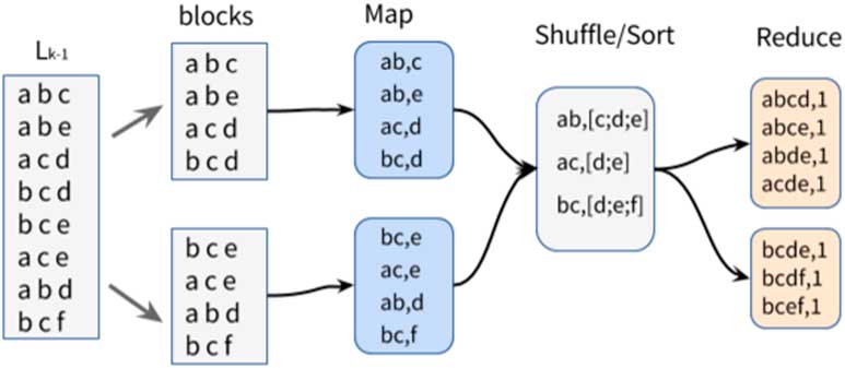
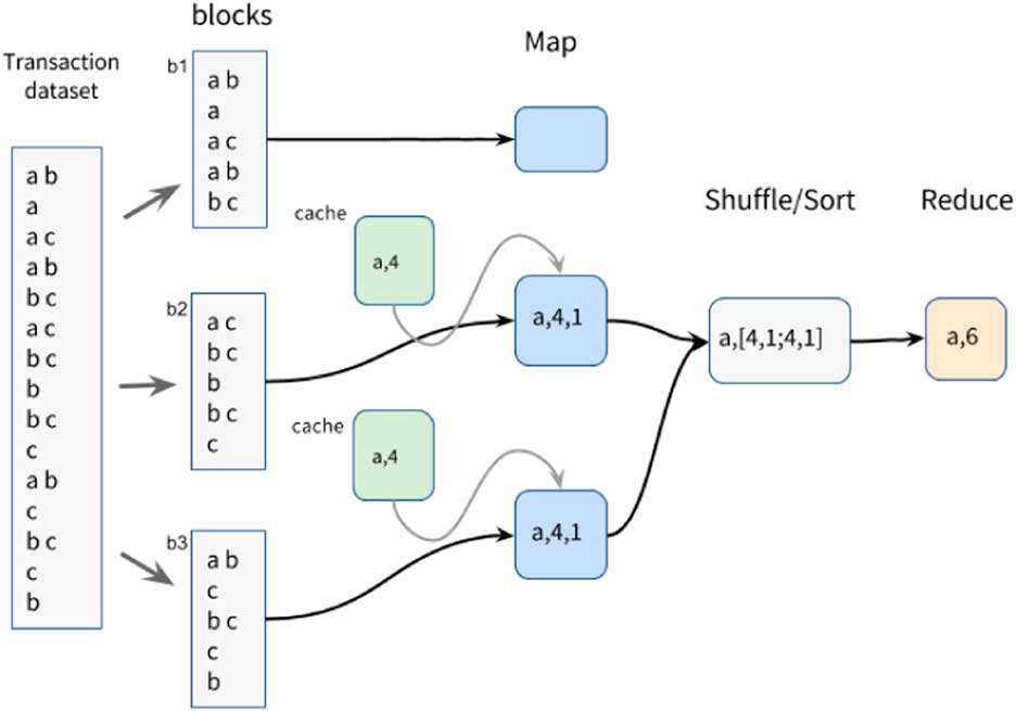
The IMRAprioriAcc algorithm also uses the same partitioning scheme of input transactions in blocks for the Map functions. However, unlike the other two algorithms, all processing is done in only two phases. Each Map function in Phase 1 performs all the steps of generating frequent itemsets for its input transaction block, considering a partial minimum support. An example is shown in Figure 3. The Reduce function returns the globally frequent itemsets and marks the partially frequent ones to be counted again in Maps where they were not frequent. Phase 2 then performs this re-count and frequency check, as illustrated by the example in Figure 4.
Example of Phase 1 of Improved MapReduce Apriori Accelerated with minimum support equal to 6 (40%)

Example of Phase 2 of Improved MapReduce Apriori Accelerated with minimum support equal to 6 (40%)

IMRAprioriAcc reduces the number of phases, consequently the time spent with communication among iterations, however, the parallelism occurs only at the level of partitioning of the input transactions. The CPA has the largest number of MapReduce iterations, however, it has the highest degree of parallelism, which can compensate for the communication time.
4 Apriori implementations on Spark
In this work, we have adapted IMRAprioriAcc, DPC and CPA approaches, originally proposed for Hadoop-MapReduce, to run on Spark framework, in order to determine whether there is a significant improvement of these approaches when running in the framework that keeps data in memory. The algorithms follow the same strategies of its original Hadoop-MapReduce implementations, except that data are kept in memory during the iterative process, by using RDDs.
In addition, we propose a new Apriori implementation to Spark, which incorporates some strategies of the three other approaches. These implementations are detailed in the following sections.
4.1 Adaptations of Hadoop-MapReduce approaches to Spark
Following, we present the adaptations of the IMRAprioriAcc, DPC and CPA approaches to run on Spark.
4.1.1 IMRAprioriAcc Spark
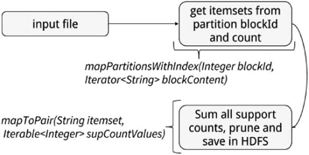
In the implementation of IMRAprioriAcc on Spark, the function mapPartitionWithIndex() is used in both phases, which identifies which block is currently being processed, making it possible to identify the source block of a given itemset. The execution flow of IMRAprioriAcc Phase 1 on Spark is shown in Figure 5. It applies the function mapPartitionWithIndex() on the transaction data set, using ID and the block content as parameters. Then, all partially frequent itemsets are generated. After that, it performs the function mapToPair() using the itemset and its list of support counters as parameters, in order to separate the globally frequent and the partially frequent itemsets, which still need to be counted in Phase 2.
Flow of Phase 1—Improved MapReduce Apriori Accelerated Spark

In Phase 2, the support of partially frequent itemsets are counted by the function mapPartitionWithIndex(), which count them only in the partitions where they were not partially frequent. In addition to the block with transactions, this function retrieves the list of itemsets that must be counted in the specific partition. Then the function mapToPair() to count globally each itemset is applied. The flow of this implementation is illustrated in Figure 6.
Flow of Phase 2—Improved MapReduce Apriori Accelerated Spark

4.1.2 DPC Spark
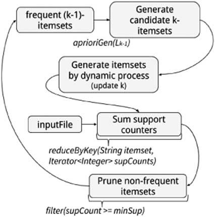
The execution flow of DPC on Spark for generating itemsets of sizes 1 and 2 is shown in Figure 7. From the itemsets of size 3, it is carried an iterative and dynamic process to produce the other frequent itemsets, as shown in Figure 8. The dynamic process for generating itemsets is similar to that implemented in the Hadoop-MapReduce version of the algorithm.
Flow of Phases 1 and 2—Dynamic Passes Combined-Counting Spark

Flow of the dynamic phase—Dynamic Passes Combined-Counting Spark

4.1.3 CPA Spark
CPA was implemented on Spark following the same strategy adopted on Hadoop-MapReduce. For generating frequent itemsets of sizes 1 and 2, the process is similar to that of Phases 1 and 2 of DPC. From the generation of candidate itemsets of size 3, the iterative process for generating candidates and counting/pruning for producing frequent itemsets starts, as shown in Figure 9.
Flow for Complete Parallel Apriori Spark

4.2 New approach IMRAprioriAcc-CPA Spark
In our experiments, we have found that IMRAprioriAcc’s strategy is efficient for small data sets. It optimizes data computing by processing only itemsets that are likely to be frequent across all partitions. However, for large data sets, processing takes a long time because the algorithm processes the entire dataset in only two phases. On the other hand, CPA presents good results for large data sets, since it parallels the generation of candidate itemsets. Our hypothesis is that the combination of the two algorithms could yield good results.
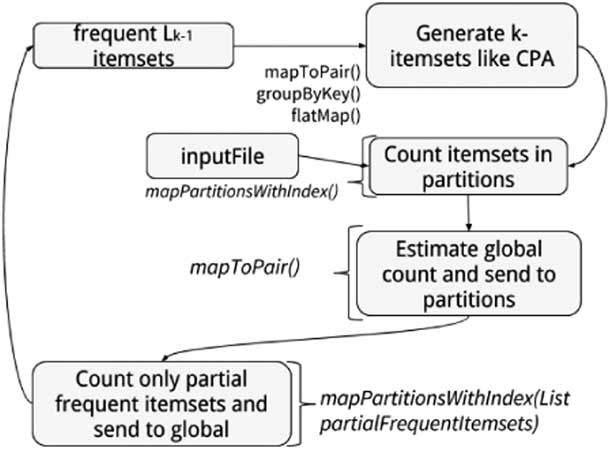
Thus, we propose an approach, called IMRAprioriAcc-CPA Spark, which is an iterative version for Spark with k phases, where each phase processes only itemsets of size k using the IMRAprioriAcc Spark strategy to find the frequent itemsets and CPA Spark strategy for generating candidate itemsets in parallel.
The first two iterations are for generating frequent itemsets of sizes 1 and 2, respectively. The flow of these two first steps are similar to IMRAprioriAcc Spark, except that instead of generating all partially frequent itemsets, it produces only the itemsets of size 1 in the first iteration and of size 2 in the second iteration. The itemsets are kept in RDD rather than save them on disk. Each iteration estimates the global support of itemsets that are not frequent in all blocks and performs the counting of partially frequent itemsets. From the itemsets of size 3, it uses the CPA strategy for generating candidate itemsets. Then, the IMRAprioriAcc strategy for counting and pruning is applied in order to produce frequent itemsets. The flow of this process is shown in Figure 10. Iterations finalize when it is no longer possible to produce frequent itemsets.
Flow for Improved MapReduce Apriori Accelerated-Complete Parallel Apriori Spark

5 Experimental evaluation
In order to evaluate the hypothesis of this work, a series of experiments are performed, comparing the various implementations of Apriori on Hadoop-MapReduce and Spark for different datasets, minimal support and number of machines in the cluster.
Runtime is used as an evaluation metric. Each run is performed three times, and the time reported herein is the average of three runs.
We have also evaluated the metrics SpeedUp, SizeUp and ScaleUp. SpeedUp evaluates algorithm performance by running the same dataset while varying the number of machines that process it, as shown in Equation (3), where T 1 is the algorithm runtime with one machine and T p the algorithm runtime with p machines.
 $$SpeedUp{\equals}{{T_{1} } \over {T_{p} }}$$
SizeUp evaluates the algorithm performance when only the data set increases, while the number of machine processing them remains constant, as shown in Equation (4), where T m is the runtime with m×data and T 1 the runtime to process data.
 $$SizeUp(data,m){\equals}{{T_{m} } \over {T_{1} }}$$
ScaleUp evaluates the algorithm performance when both the dataset to be processed increases and, proportionally, the number of machines processing these data also increases. Equation (5) shows the calculation of ScaleUp, where T 1 is the runtime to process data in one machine and T mm the runtime to process m×data in m machines.
 $$ScaleUp(data,m){\equals}{{T_{1} } \over {T_{{mm}} }}$$
We use eight synthetic data sets produced by the library ‘arules’ (Hahsler et al., Reference Dean and Ghemawat2016) of R-cran Software. The data sets T30D1000K10K and T15D1000K100K are those generating more computational processing due to higher number of items per transaction. Table 1 presents the characteristics of our data sets.
Data sets

All experiments were run on a cluster of computers with 20 machines, one exclusive to master and 19 slaves. Each machine has Intel Core i5-2400 processor with four 3.10 GHz processor cores, 8GB of RAM and 500GB HD. All running Ubuntu Desktop operating system 14.04 LTS, Hadoop 2.7.1 and Spark 1.5.2.
As statistical test, we have performed the t-test to verify if there is statistical significant difference among the runtime in the comparison of the algorithms. At all points in the following text, where one algorithm is said to be better than another, this was statistically verified with 95% confidence (p-value<0.05).
In the following, we present the results and analysis of the experiments.
5.1 Comparison of Hadoop-MapReduce algorithms
For the three implementations of Apriori algorithm on Hadoop-MapReduce, experiments are performed using eight Maps, eight Reduces and three distinct values of minimum support: 0.5, 0.1 and 0.01%. Among them, 0.5 and 0.1% are the values most commonly used in the literature, and 0.01% have been chosen to generate a greater amount of itemsets, and thereby to assess how efficient are the implementations of 2 and k phases.
For the minimal support 0.5% (0.005), the three algorithms have presented a similar pattern of behavior for all datasets, with IMRAprioriAcc being the fastest, followed by DPC and CPA. Figure 11 shows the execution time for the three algorithms in all data sets. For this support, the amount of frequent itemsets produced is relatively small, about 16 M frequent itemsets to the data set that produced more itemsets (T30D1000KN10K) and about 120 for the data set that produced fewer itemsets (T5D1000KN100K).
Runtime for the algorithms for minimum support 0.5%, eight Maps and eight Reduces. IMRAprioriAcc=Improved MapReduce Apriori Accelerated; DPC=Dynamic Passes Combined-Counting; CPA=Complete Parallel Apriori

For the data set that produced fewer itemsets, IMRAprioriAcc is 83% faster than DPC and 203% faster than CPA, while DPC is 65% faster than CPA. For the data set that produced more itemsets, IMRAprioriAcc is 430% faster than DPC and 488% faster than CPA, while DPC is 11% faster than CPA.
This great difference in behavior of the algorithms of k phases in relation to the two-phase algorithm is mainly due to the larger number of necessary MapReduce executions to find all frequent itemsets. For the smallest data set, DPC has spent three MapReduce executions while CPA spent seven. For the largest data set, DPC has spent five executions and CPA 18. Despite having spent more MapReduce executions than DPC, CPA is only 11% slower for the largest data set related to the smallest. The reason is that in the dynamic phases of DPC, the candidate k-itemsets are produced from the (k−1)-itemsets also candidates (not by using the frequents as in CPA). This results in a lot of false candidate itemsets being processed, damaging the runtime. For example, Phase 4 of DPC has generated itemsets of sizes 4, 5 and 6. Candidate 4-itemsets are generated from the frequent 3-itemsets of the previous phase, but candidate 5-itemsets are generated from these candidate 4-itemsets. The same goes for the candidate 6-itemsets, which is generated from the candidate 5-itemsets. Only after the generation of candidates, the counting and pruning occurs to produce the frequent 4, 5 and 6-itemsets.
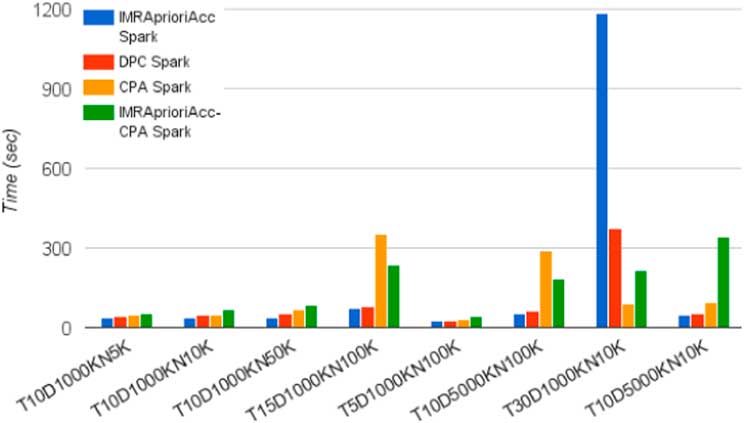
For the minimum support 0.1% (0.001), the algorithms runtime tend to exhibit the same behavior in relation to the minimum support 0.5%, except for the largest data set, T30D1000KN10K, where CPA has obtained the best performance. Figure 12 shows the results for this configuration. CPA is 25% faster than IMRAprioriAcc and 41% faster than DPC. While IMRAprioriAcc is 13% faster than DPC. For this data set, 88 295 frequent itemsets with size from k=1 to k=10 have been generated. Remember that IMRAprioriAcc generate all candidate and frequent itemsets in only two phases, with an emphasis in Phase 1 where all combinations of items are generated. In Phase 1, the time consumption was 99.89% of the total running time of IMRAprioriAcc. It is a process that requires a long time, because in this phase itemsets of 10 different sizes are produced in each Map function.
Runtime for the algorithms for minimum support 0.1%, eight Maps and eight Reduces. IMRAprioriAcc=Improved MapReduce Apriori Accelerated; DPC=Dynamic Passes Combined-Counting; CPA=Complete Parallel Apriori

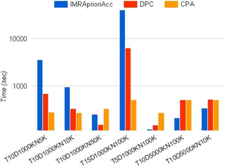
For the minimum support 0.01% (0.0001), memory overflow problems have been observed for the largest data set, because the volume of processed itemsets is quite high. For the other data sets, CPA is the fastest in four of them, as shown in Figure 13. In addition, DPC has also presented better results than IMRAprioriAcc in some data sets. For example, on T15D1000KN100K data set, CPA runtime is 541% faster than DPC, and 7987% faster than IMRAprioriAcc. For this data set, 390 769 frequent itemsets have been generated with size from k=1 to k=13, resulting in 25 MapReduce executions to CPA and six to DPC. Despite the amount of MapReduce executions, CPA processes relatively fewer itemsets per executions than DPC, which makes all the time spent on startup and Hadoop communication negligible. Note that as the number of frequent itemsets produced increases, the algorithms with fewer MapReduce executions tend to demand more runtime.
Runtime for the algorithms for minimum support 0.01%, eight Maps and eight Reduces. IMRAprioriAcc=Improved MapReduce Apriori Accelerated; DPC=Dynamic Passes Combined-Counting; CPA=Complete Parallel Apriori

5.1.1 SpeedUp
The graphic of SpeedUp experiments is shown in Figure 14. It was used the data set T10D1000KN10K with minimum support 0.01%. Note that the DPC has presented the most SpeedUp for up to four machines. From that on, it tends to stabilize. CPA has presented a steadier growth, decreasing after eight machines. IMRAprioriAcc, on the other hand, has presented worsening in performance as the number of machines increased. This occurs because of the control that the algorithm must keep on data partitions around the cluster to its counting and pruning process. The greater the number of partitions, the more disk I/O operations are required in the execution of the algorithm.
SpeedUp for the Hadoop-MapReduce algorithms. IMRAprioriAcc=Improved MapReduce Apriori Accelerated; DPC=Dynamic Passes Combined-Counting; CPA=Complete Parallel Apriori

5.1.2 SizeUp
The graphic of SizeUp experiments is shown in Figure 15. Eight slave machines were kept in the cluster, while the number of transactions, with minimum support 0.1%, has increased the data set. It is noted that the algorithms tend to lose performance as the data set grows from 2 million to 4 million, especially DPC has had the worst performance on SizeUp among the three algorithms.
SizeUp for the Hadoop-MapReduce algorithms. IMRAprioriAcc=Improved MapReduce Apriori Accelerated; DPC=Dynamic Passes Combined-Counting; CPA=Complete Parallel Apriori

Phases 2 and 4 of DPC demand more time and processed more itemsets. Phase 2 requires more time to find all the frequent 2-itemsets, and Phase 4 produces more itemsets. This means that, in some cases, the dynamic approach is not so efficient, since it may cause bad distribution load between phases, causing overheads in parallelization, which impacts on the final runtime.
5.1.3 ScaleUp
The graphic of ScaleUp experiments is shown in Figure 16, also using the minimum support 0.1%. It is possible to note that IMRAprioriAcc and DPC have low scalability compared to CPA. From eight machines, DPC has worsened scalability getting down 60%, while CPA and IMRAprioriAcc are above 70%.
ScaleUp for the Hadoop-MapReduce algorithms. IMRAprioriAcc=Improved MapReduce Apriori Accelerated; DPC=Dynamic Passes Combined-Counting; CPA=Complete Parallel Apriori

5.2 Comparison of Spark algorithms
For the four Apriori algorithm implementations on Spark the data sets of the experiments have been divided into eight blocks (eight machines) and, as on Hadoop-MapReduce, three different values of minimum support have been used, namely 0.5, 0.1 and 0.01%.
Figure 17 presents the runtime for Spark algorithms, using minimum support 0.5% (0.005). At this level of support, the algorithms are statistically tied, although IMRAprioriAcc Spark and DPC Spark are numerically better in some data sets.
Runtime for the Spark algorithms for minimum support 0.5% and eight blocks. IMRAprioriAcc=Improved MapReduce Apriori Accelerated; DPC=Dynamic Passes Combined-Counting; CPA=Complete Parallel Apriori

The results also show that the new approach, IMRAprioriAcc-CPA Spark, is not suitable for experiments with this minimum level of support, because despite being an algorithm of k phases, it performs many operations per phase, mixing the pruning strategy of IMRAprioriAcc-Spark and the generation of candidates of CPA-Spark. Then, for situations with few itemsets produced, these operations cannot be efficient.
For minimum support 0.1% (0.001), IMRAprioriAcc Spark is the fastest algorithm for five data sets, followed by DPC Spark, CPA Spark and CPA-IMRAprioriAcc Spark, as shown in Figure 18. Only for the largest data set (T30D1000KN10K) variation of the fastest algorithm has been observed. For this data set, CPA Spark is the fastest, and IMRAprioriAcc Spark the slowest algorithm, being 1231% slower. It is noted a similar behavior on Hadoop-MapReduce algorithms as the minimum support decreases. IMRAprioriAcc-CPA Spark is the second fastest to that data set.
Runtime for the Spark algorithms for minimum support 0.1% and eight blocks. IMRAprioriAcc=Improved MapReduce Apriori Accelerated; DPC=Dynamic Passes Combined-Counting; CPA=Complete Parallel Apriori

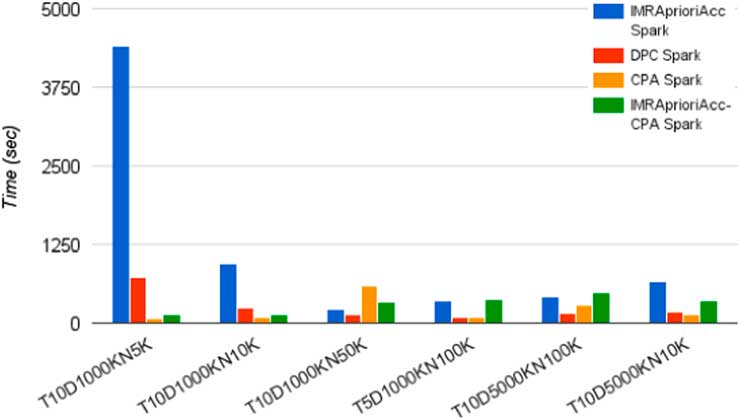
For minimum support 0.01% (0.0001), the amount of itemsets produced for each data set is very large, resulting in execution problems on Spark algorithms for some data sets, due to memory limit of each machine. Therefore, it has not been possible to obtain the results for some data sets due to the high demand for memory. For the processed data sets, it is observed that CPA Spark is the fastest algorithm for the four of them, and DPC Spark for two other data sets, as shown in Figure 19. IMRAprioriAcc Spark, by performing only two iterations, the same as in its implementation on Hadoop-MapReduce, is the slowest of the four algorithms, being 6038% slower than CPA Spark for the T10D1000KN5K data set. DPC Spark and IMRAprioriAcc-CPA Spark are 921 and 78% slower than CPA Spark, respectively, for the same data set. As noted in Hadoop-MapReduce algorithms, as the amount of produced frequent itemsets increases, Spark algorithms with fewer iterations tend to demand more runtime.
Runtime for the Spark algorithms for minimum support 0.01% and eight blocks. IMRAprioriAcc=Improved MapReduce Apriori Accelerated; DPC=Dynamic Passes Combined-Counting; CPA=Complete Parallel Apriori

5.2.1 SpeedUp
The graphic of SpeedUp experiments is shown in Figure 20. As for the Hadoop-MapReduce algorithms, data set T10D1000KN10K and minimum support 0.01% are used. Note that with two machines the new approach has presented the best SpeedUp performance. With four machines, IMRAprioriAcc-CPA Spark and CPA Spark have SpeedUp drop. Both use the same method for generating candidate itemsets, which implies more data transferring through the network. With eight machines, the amount of data transferring between each machine is reduced, decreasing overloading on the network and increasing the SpeedUp rate. With 16 machines, CPA Spark has obtained the best SpeedUp, while IMRAprioriAcc Spark has presented a similar behavior to its implementation on Hadoop-MapReduce. Overall, the Hadoop-MapReduce algorithms have presented better SpeedUp, except for IMRAprioriAcc.
SpeedUp for Spark algorithms. IMRAprioriAcc=Improved MapReduce Apriori Accelerated; DPC=Dynamic Passes Combined-Counting; CPA=Complete Parallel Apriori

5.2.2 SizeUp
The graphic of SizeUp experiments, using minimum support 0.1%, is shown in Figure 21. Note that IMRAprioriAcc-CPA Spark has presented the best SizeUp among the four algorithms, that is, the algorithm is more efficient than the others as the data set grows. For this case, CPA Spark has low performance for data sets with 2 million transactions, while IMRAprioriAcc Spark is the worst one for the data set of 4 million transactions. Despite IMRAprioriAcc-CPA Spark spending the same amount of iterations as CPA Spark, its counting and pruning of itemsets method is more efficient, which contributes to its best performance. Spark approaches has overcame the Hadoop-MapReduce algorithms in SizeUp.
SizeUp for Spark algorithms. IMRAprioriAcc=Improved MapReduce Apriori Accelerated; DPC=Dynamic Passes Combined-Counting; CPA=Complete Parallel Apriori

5.2.3 ScaleUp
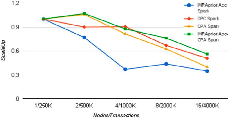
The graphic of ScaleUp experiments, using minimum support 0.1%, is shown in Figure 22. IMRAprioriAcc-CPA Spark has presented an interesting behavior, it remains better than the other approaches for almost every situation. Except in the case of four machines and data set of 1 million transactions, where DPC Spark is slightly better. IMRAprioriAcc Spark has presented the worst performance for ScaleUp, keeping around 40% or less for 4, 8 and 16 machines.
ScaleUp for Spark algorithms. IMRAprioriAcc=Improved MapReduce Apriori Accelerated; DPC=Dynamic Passes Combined-Counting; CPA=Complete Parallel Apriori

For ScaleUp, Hadoop-MapReduce approaches have better behavior than Spark algorithms, especially when the number of machines and size of the data set are higher.
5.3 Comparison Hadoop-MapReduce vs. Spark algorithms
In all experiments, there is at least one Spark algorithm that is faster than all Hadoop-MapReduce algorithms. However, Spark implementations have more limitations due to the size of available memory. For cases where many frequent itemsets are generated (≈200 K), CPA Hadoop-MapReduce have had the best performance. When the amount of produced frequent itemsets is between 50 K and 200 K, CPA Spark is the most efficient. Between 10 and 50 K, IMRAprioriAcc Spark is the best option. Below that, DPC Spark is the algorithm with the best performance. Figure 23 presents a summary of the results, according to the amount of produced frequent itemsets. Note that for the four situations (low, middle-low, middle-high and high itemsets amounts), three of the algorithms with the best performance are Spark, while CPA Hadoop-MapReduce has obtained the best results for the highest itemsets amount.
Summary of cases where each algorithm had the best performance, based on the amount of frequent itemsets. IMRAprioriAcc=Improved MapReduce Apriori Accelerated; DPC=Dynamic Passes Combined-Counting; CPA=Complete Parallel Apriori

6 Framework for algorithm recommendation
According to the results of the experiments, we present, by Algorithm 12, a framework to recommend the best implementation for each execution, according to data set features, minimum required support, and size of the main memory available per machine. The recommendation is based on the potential for generating frequent itemsets, generalizing the data from our experiments.
Our recommendation is divided in three levels of minimum support. For the highest values (higher than 0.5), we recommend to use IMRAprioriAcc Spark. For intermediate values (between 0.05 and 0.5), if the data set has a few items per transaction, we also recommend IMRAprioriAcc Spark. For more items per transaction, we recommend CPA Spark where are at least 8GB of main memory available per machine or, to the contrary, we recommend CPA on Hadoop-MapReduce. For the lowest minimum support values (less than 0.05), if there is enough memory or a few items per transaction, we recommend CPA Spark, to the contrary, we recommend CPA on Hadoop-MapReduce.

We have experimentally evaluated our proposed framework on two synthetic data sets, T10D2000KN10K and T40D1000KN10K, and on two real data sets available at fimi.ua.ac.be, ‘retail.dat’ and ‘kosarak.dat’, for four values of minimum support, 1, 0.2, 0.07 and 0.005%. The retail.dat data set has 88.162 transactions, 16.470 distinct items and 10 items per transaction. kosarak.dat has 990.002 transactions, 41.270 distinct items, and eight items per transaction. The results indicate the correct paths of our framework, where CPA Spark is the most appropriate algorithm for data sets with more than 20 items per transaction or low support.
7 Conclusions and future work
In this work, we have performed a detailed study of several Apriori algorithm implementations for the Hadoop-MapReduce framework, as well as their adaptation to Spark framework. We have compared implementations that produce frequent itemsets in two or k phases, where each phase is a MapReduce iteration. Implementations have been compared using different values for the minimum support and different data sets, varying the amount of transactions, the number of distinct items and the number of items per transaction.
For Hadoop-MapReduce, we observe that when the amount of produced frequent itemsets is low, IMRAprioriAcc, which is a two-phase algorithm, obtains better performance than other k phases approaches. On the other hand, CPA is the best implementation for large amounts of produced itemsets. CPA is also the implementation with the best scalability.
For Spark, the adapted algorithms perform similarly to Hadoop-MapReduce, except that DPC also performes well when the amount of frequent itemsets is low. CPA, which has the best performance for large amounts of frequent itemsets, presents unstable scalability.
Comparing performance of the algorithms between Hadoop-MapReduce and Spark, Spark implementations have obtained better performance. However, Spark uses RDDs that keep data in memory, and thus, when the amount of memory in the cluster machines is no longer sufficient to process large data sets, it is recommended to use the implementation of CPA for Hadoop-MapReduce.
As a result of the evaluation, we have produced a framework to recommend the algorithm to be applied by users according to the features of the data set and the desired minimum support value.
As future work, we intend to develop a strategy that takes advantage of the good performance of Spark, but to also be able to store data on disk when processing in memory is a limitation. Moreover, we are mapping algorithms for associative classification (Wedyan, Reference Yahya, Hegazy and Ezat2014) to Hadoop-MapReduce and Spark, in particular we are mapping an algorithm for classifying product offers from e-shoppings (Oliveira & Pereira, Reference White2017).
Acknowledgments
This work was partially supported by CNPq, FAPEMIG grant CEX-APQ-01834-14 and an individual scholarship from CAPES.