1 Introduction
Scalar contaminants such as toxic gases and pollutants are often inadvertently introduced into a background flow (e.g. in the atmosphere boundary layer) approximately at a point, or at source sizes that are significantly smaller compared to the domain of bulk flow. Dispersion of a passive scalar released from a point source in a turbulent boundary layer encompasses many features of atmospheric flows, and is the focus of this study. The transport of a scalar in a turbulent flow depends on both the instantaneous as well as the time-averaged properties of the scalar and the flow itself. This is clearly evident in the Reynolds-averaged mean scalar and scalar-variance equations,
 $$\begin{eqnarray}\displaystyle & \displaystyle U_{i}\frac{\unicode[STIX]{x2202}C}{\unicode[STIX]{x2202}x_{i}}=-\frac{\unicode[STIX]{x2202}\,\overline{u_{i}c}}{\unicode[STIX]{x2202}x_{i}}+D(\unicode[STIX]{x1D6FB}^{2}C), & \displaystyle\end{eqnarray}$$
 $$\begin{eqnarray}\displaystyle & \displaystyle U_{i}\frac{\unicode[STIX]{x2202}\,\overline{cc}}{\unicode[STIX]{x2202}x_{i}}=-\frac{\unicode[STIX]{x2202}\,\overline{u_{i}cc}}{\unicode[STIX]{x2202}x_{i}}+D(\unicode[STIX]{x1D6FB}^{2}\,\overline{cc})-2\overline{u_{i}c}\,\frac{\unicode[STIX]{x2202}C}{\unicode[STIX]{x2202}x_{i}}-\unicode[STIX]{x1D712}_{c}, & \displaystyle\end{eqnarray}$$
 $\tilde{\boldsymbol{U}}=\tilde{U}\hat{\boldsymbol{i}}+\tilde{V}\hat{\boldsymbol{j}}+\tilde{W}\hat{\boldsymbol{k}}$
) and the scalar fields. Here, the instantaneous streamwise velocity and concentration are denoted as
 $\tilde{U}=U+u$
and
 $\tilde{C}=C+c$
, respectively,
 $D$
represents the coefficient of molecular diffusion and
 $\unicode[STIX]{x1D712}_{c}=2D\overline{(\unicode[STIX]{x2202}c/\unicode[STIX]{x2202}x_{i})(\unicode[STIX]{x2202}c/\unicode[STIX]{x2202}x_{i})}$
is the rate of dissipation of scalar variance. Note that upper-case letters or the overline represent the time-averaged (mean) quantities, whereas the corresponding lower-case letters denote the fluctuating quantities defined about the mean. Thus an understanding of instantaneous processes within a plume is essential for establishing a description of the physics that controls the time-averaged properties.
Several past studies have examined scalar dispersion and also developed statistical models for its prediction in both convective boundary layers (see Townsend Reference Townsend1958; Arya Reference Arya1975; Willis & Deardorff Reference Willis and Deardorff1978; among others) and rough-wall turbulent boundary layers (Poreh & Cermak Reference Poreh and Cermak1964; Fackrell & Robins Reference Fackrell and Robins1982; Sawford, Frost & Allan Reference Sawford, Frost and Allan1985; Yee et al. Reference Yee, Kosteniuk, Chandler, Biltoft and Bowers1993; Nironi et al. Reference Nironi, Salizzoni, Marro, Mejean, Grosjean and Soulhac2015). However, there are no known studies of scalar dispersion in canonical smooth-wall turbulent boundary layers. The emphasis on rough-wall boundary layers is understandable since atmospheric flows are characteristically developing over some form of roughness. One of the aims of the current study is to fill this gap of experiments over smooth walls and to associate the substantial knowledge of turbulence structure in wall-bounded flows with dispersion. Thereby, we also aim to understand the influence of coherent motions in boundary layer flows on scalar transport, as such motions also play an important role in the transport of momentum and vorticity across the boundary layer (Marusic et al. Reference Marusic, McKeon, Monkewitz, Nagib, Smits and Sreenivasan2010; Smits, McKeon & Marusic Reference Smits, McKeon and Marusic2011; Klewicki Reference Klewicki2013).
For a plume released from a point source, Fackrell & Robins (Reference Fackrell and Robins1982) and Nironi et al. (Reference Nironi, Salizzoni, Marro, Mejean, Grosjean and Soulhac2015), both using the flame ionisation detection technique for measuring instantaneous concentration, have shown that the mean and variance of concentration fluctuations in a rough-wall turbulent boundary layer exhibit either reflected Gaussian or Gaussian behaviour depending on the source height. Fackrell & Robins (Reference Fackrell and Robins1982) found that a ground-level plume tends to disperse in a Gaussian distribution (to a close approximation) while an elevated plume exhibits a reflected Gaussian behaviour, which has been further substantiated by Nironi et al. (Reference Nironi, Salizzoni, Marro, Mejean, Grosjean and Soulhac2015). Both these studies considered a ground-level and a single elevated source and thus could not clarify the influence of source height on plume dispersion. To this end, the current study reports experimental data for different source heights in the near-wall region, log layer, fully turbulent outer region and intermittent region of a boundary layer.
Another parameter relevant to plume dispersion is the source size (Chatwin & Sullivan Reference Chatwin and Sullivan1979; Durbin Reference Durbin1980). The influence of source size can be examined by considering the Gaussian plume model put forth by Gifford (Reference Gifford1959). He suggested that the concentration fluctuations are governed by two distinct phenomena – meandering of the instantaneous plume and relative dispersion of the plume particles. In general, the meandering is due to the presence of wide range of length scales in the flow relative to the source size. Using the results of Hay & Pasquill (Reference Hay and Pasquill1959) and Smith & Hay (Reference Smith and Hay1961) on relevant scales for plume dispersion, Fackrell (Reference Fackrell1980) showed that meandering is the major source of concentration fluctuations in a developing plume. Experimental studies (Fackrell & Robins Reference Fackrell and Robins1982; Nironi et al.
Reference Nironi, Salizzoni, Marro, Mejean, Grosjean and Soulhac2015) have concluded that the source size does not influence a ground-level plume since the turbulent length scales near the wall are typically smaller than or comparable to the source size. On the other hand, the source diameter influences the structure of an elevated plume, as the turbulent eddies are nominally larger than the source diameter. For an elevated source, the results from (Fackrell & Robins Reference Fackrell and Robins1982; Nironi et al.
Reference Nironi, Salizzoni, Marro, Mejean, Grosjean and Soulhac2015) conclusively show that the variation of source size does not alter the mean concentration field but affects the concentration fluctuations, which is the case in the current study, i.e.
 $s_{d}/\unicode[STIX]{x1D6FF}\approx 0.0025$
, where
 $s_{d}$
is the source diameter.
The seminal study of Taylor (Reference Taylor1921) shows that the spread of a scalar depends on the Lagrangian integral time scales in the flow, and since then there have been efforts to estimate them using the Eulerian integral time scales (
 $\unicode[STIX]{x1D70F}_{c}$
), which are experimentally more easily tractable. Eulerian autocorrelation functions and corresponding time scales are important quantities in their own right, and a few studies, such as Antonia, Danh & Prabhu (Reference Antonia, Danh and Prabhu1977), Tavoularis & Corrsin (Reference Tavoularis and Corrsin1981) and Krishnamoorthy & Antonia (Reference Krishnamoorthy and Antonia1987), have employed temperature as a passive scalar using coldwires (with constant current anemometry) to measure temperature fluctuations with high temporal resolution. Although temperature is a suitable passive scalar, it is challenging to implement its release from a source in close vicinity of a surface due to conduction at physical boundaries, i.e. the boundary condition of zero flux at the wall,
 $\text{d}\tilde{C}/\text{d}z=0$
at
 $z=0$
, cannot be ensured (
 $z$
is the distance from the wall). On the other hand, the use of gas as a passive scalar does not suffer this limitation due to non-permeability of the wall. However, measuring gas concentration at high frequency is difficult, and currently available instrumentation such as flame ionisation detectors (FID) and photoionisation detectors (PID) have typical response of up to 400 Hz. Further, these sensors are prone to drift in time due to humidity, variation in temperature and changes in background concentration of the flow. To minimise the effect of sensor drift on statistics, we have successfully implemented systematic calibration procedures (Talluru et al.
Reference Talluru, Hernandez-Silva, Philip and Chauhan2017a
) for photoionisation detectors (which could also be implemented for flame ionisation detectors), and consequently an accurate computation of
 $\unicode[STIX]{x1D70F}_{c}$
is possible, the results of which will be presented here. Fackrell & Robins (Reference Fackrell and Robins1982) is the only study, to our knowledge, that has reported the statistics of
 $\unicode[STIX]{x1D70F}_{c}$
for ground-level and elevated plumes and observed that
 $\unicode[STIX]{x1D70F}_{c}$
is higher near the wall. Further, with only few measurement points across the plume, they found that there is little variation of
 $\unicode[STIX]{x1D70F}_{c}$
vertically for an elevated source. Here, we aim to document the behaviour of
 $\unicode[STIX]{x1D70F}_{c}$
across the plume from a point source released at various heights, and to understand its variation.
In the past few decades, numerous studies have also reported the presence of coherent structures in various turbulent flows and, more recently, these structures have been identified to contribute to the generation of Reynolds stresses, which play a dominant role in the transport of momentum. There is evidence that coherent motions are responsible for heat and momentum fluxes in the atmospheric surface layer (Katul et al. Reference Katul, Kuhn, Schieldge and Hsieh1997; Finnigan, Shaw & Patton Reference Finnigan, Shaw and Patton2009; Li & Bou-Zeid Reference Li and Bou-Zeid2011; Huang, Katul & Albertson Reference Huang, Katul and Albertson2013). Further, from the presence of mean and fluctuation velocity in (1.1a ) and (1.1b ), it follows that coherent structures would also be significant for scalar transport. However, the exact nature of scalar transport by coherent features is not well understood, possibly due to experimental complexity in obtaining simultaneous measurements of velocity and concentration with good spatial and temporal resolution. Recently Vanderwel & Tavoularis (Reference Vanderwel and Tavoularis2016) observed that a scalar dye segregated preferentially within vortex cores and the boundaries of uniform-momentum zones (see Meinhart & Adrian (Reference Meinhart and Adrian1995) for a description of uniform-momentum zones) in a uniformly sheared flow. Vanderwel & Tavoularis (Reference Vanderwel and Tavoularis2016) also utilised conditional analysis to show that strong scalar flux events are well correlated with Reynolds shear stress events. Thus it is imperative to understand transport of a scalar by known coherent features such as hairpin packets (e.g. Adrian, Meinhart & Tomkins Reference Adrian, Meinhart and Tomkins2000), meandering superstructures (e.g. Hutchins & Marusic Reference Hutchins and Marusic2007a ), vortical motions (e.g. Klewicki, Murray & Falco Reference Klewicki, Murray and Falco1994; Herpin et al. Reference Herpin, Stanislas, Foucaut and Coudert2013) and uniform-momentum zones (e.g. de Silva et al. Reference de Silva, Philip, Hutchins and Marusic2017). Here, analysis of cross-correlation and cross-spectra of instantaneous velocity and concentration will provide insights into the organisation of scalar and velocity structures.
The paper is outlined as follows. Next, § 2 provides details of the experimental set-up and measurement devices. In § 3, we first present results for mean and variance of concentration as the source location is varied. This is followed by the evaluation of
 $\unicode[STIX]{x1D70F}_{c}$
and
 $\unicode[STIX]{x1D70F}_{u}$
, and spectral decomposition of scalar and velocity signals. The influence of velocity on the scalar is discussed in § 4, along with concentration flux (
 $\overline{uc}$
), cross-correlation and cross-spectral density. Further results from the joint probability density function are also included in § 4, and our phenomenological plume model to explain results and conclusions follow in § 5.
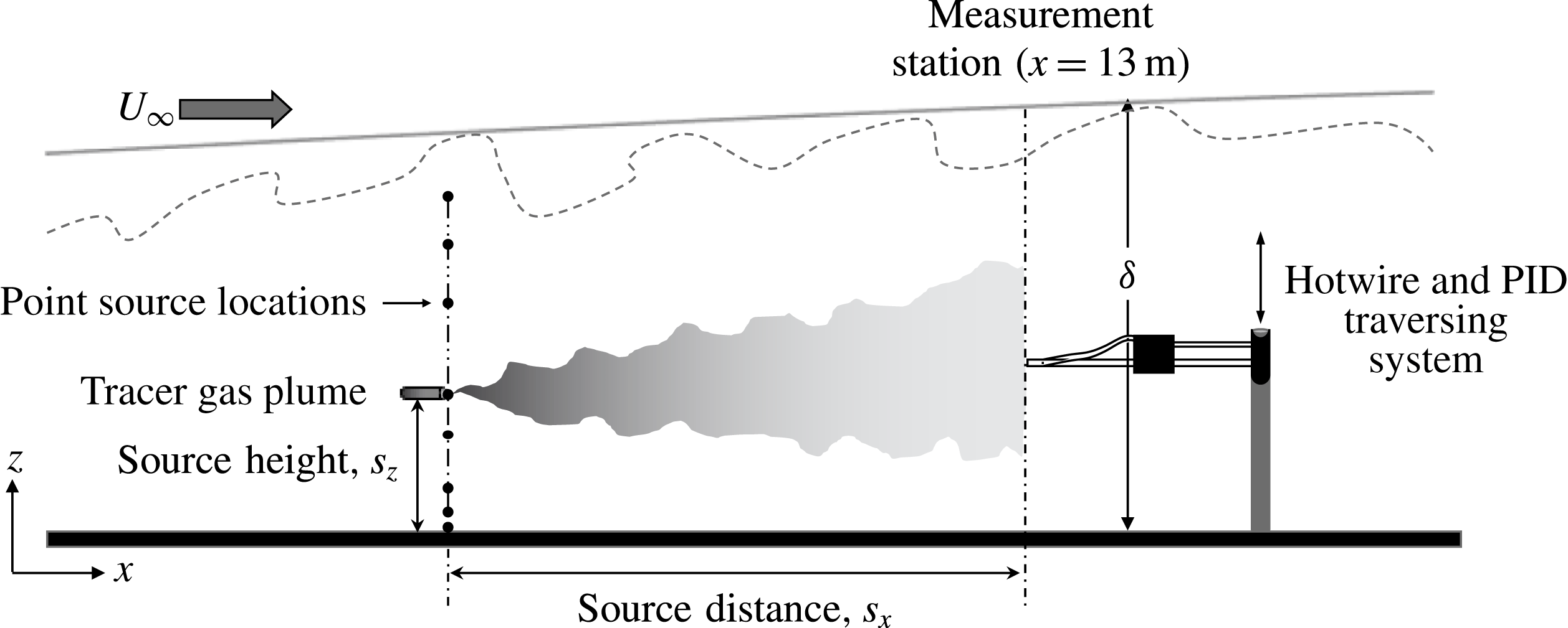
Schematic of experimental set-up showing the arrangement of hotwire and PID and different parameters of the point source.

2 Details of experiments
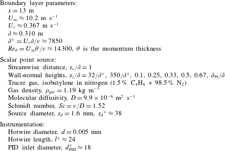
Experiments are conducted in the Boundary Layer Wind Tunnel (BLWT) located at the University of Sydney. A schematic of the experimental set-up is shown in figure 1, where simultaneous measurements of velocity and concentration are made using a single hotwire and a PID, respectively. In the present study, the free-stream velocity is set to
 $10~\text{m}~\text{s}^{-1}$
, which resulted in a boundary layer thickness
 $\unicode[STIX]{x1D6FF}\approx 0.31~\text{m}$
and friction velocity
 $U_{\unicode[STIX]{x1D70F}}\approx 0.37~\text{m}~\text{s}^{-1}$
(obtained by fitting mean velocity data to the composite velocity fit given by Chauhan, Nagib & Monkewitz (Reference Chauhan, Nagib and Monkewitz2009) using log-law constants
 $\unicode[STIX]{x1D705}=0.384$
and
 $A=4.17$
) at the measurement location
 $x=13~\text{m}$
downstream of the trip. The friction Reynolds number,
 $Re_{\unicode[STIX]{x1D70F}}\equiv \unicode[STIX]{x1D6FF}U_{\unicode[STIX]{x1D70F}}/\unicode[STIX]{x1D708}=\unicode[STIX]{x1D6FF}^{+}\approx$
7850 (
 $\unicode[STIX]{x1D708}$
is the kinematic viscosity of air) at the measurement location, and other parameters of the boundary layer are listed in table 1. Note that normalisation using wall units is denoted by a ‘
 $+$
’ superscript in this paper, e.g.
 $l^{+}=l/(\unicode[STIX]{x1D708}/U_{\unicode[STIX]{x1D70F}})$
and
 $U^{+}=U/U_{\unicode[STIX]{x1D70F}}$
, where
 $l$
is the hotwire sensor length and
 $U$
is the mean streamwise velocity. The mean velocity and turbulence intensity profiles were previously documented in (Talluru et al.
Reference Talluru, Hernandez-Silva, Philip and Chauhan2017a
), and at the measurement location closely resemble a zero-pressure-gradient turbulent boundary layer. Full details of the wind tunnel facility and the calibration procedures for PID sensors are given in Talluru et al. (Reference Talluru, Hernandez-Silva, Philip and Chauhan2017a
). In the case of hotwire measurements, procedures outlined in Talluru et al. (Reference Talluru, Kulandaivelu, Hutchins and Marusic2014) are employed to correct for any voltage drift during the measurements. Throughout this paper,
 $x$
,
 $y$
and
 $z$
refer to the streamwise, transverse and vertical directions, while
 $u$
,
 $v$
and
 $w$
denote the corresponding fluctuating velocity components.
Experimental parameters and properties of tracer gas.

A point-source tracer gas (a mixture of 1.5 % isobutylene and 98.5 % nitrogen) with an initial concentration (
 $C_{0}$
) of 15 000 ppm is released via a discharge tube at eight different heights (
 $s_{z}$
, as listed in table 1) above the tunnel floor, and measurements are made at a fixed distance
 $s_{x}/\unicode[STIX]{x1D6FF}=1$
from the source (as illustrated in figure 1). The source heights were chosen to observe variation in local spread of the scalar plume due to varying properties of local turbulence across the boundary layer. The location
 $s_{z}/\unicode[STIX]{x1D6FF}=32/\unicode[STIX]{x1D6FF}^{+}$
, which is physically
 $1.26$
mm from the ground (compared to a
 $\unicode[STIX]{x1D6FF}=310$
mm) is the closest we can release the gas and is called the ground source;
 $s_{z}/\unicode[STIX]{x1D6FF}=350/\unicode[STIX]{x1D6FF}^{+}$
and
 $s_{z}/\unicode[STIX]{x1D6FF}=0.1$
are within the inertial or log region of the boundary layer (note that the start of the log region is at
 ${\approx}3.6\sqrt{\unicode[STIX]{x1D6FF}^{+}}$
as shown recently by Morrill-Winter, Philip & Klewicki (Reference Morrill-Winter, Philip and Klewicki2017), which in our case is 319 viscous units);
 $s_{z}/\unicode[STIX]{x1D6FF}=0.25$
is in the fully turbulent outer region;
 $s_{z}/\unicode[STIX]{x1D6FF}=0.5$
is in the mostly turbulent outer region (note that external intermittency begins near
 $z/\unicode[STIX]{x1D6FF}=0.33$
(Chauhan et al.
Reference Chauhan, Philip, de Silva, Hutchins and Marusic2014b
));
 $s_{z}/\unicode[STIX]{x1D6FF}=0.67$
corresponds to a location where the flow is non-turbulent 50 % of the time; and
 $s_{z}=\unicode[STIX]{x1D6FF}_{99}$
corresponds to a location near the outer edge where the boundary layer is mostly non-turbulent.
The tracer gas is released isokinetically into the flow by matching the source velocity (
 $U_{s}$
) with the local mean velocity at
 $z=s_{z}$
, i.e.
 $U_{s}=U|_{(z=s_{z})}$
. It is important to note here that there is a time lag between the measured instantaneous velocity and concentration signals due to the delay in the response of the PID sensor compared to the hotwire. The time lag is the time required for the gas sample to travel from the sensor tip to the detection chamber of the PID. Diagnostic tests conducted by Talluru et al. (Reference Talluru, Hernandez-Silva, Philip and Chauhan2017b
) found that the PID signal has an average time lag of 10 ms with respect to the hotwire signal, and hence all the concentration signals are accordingly shifted in time for analysis. The effect of uncertainty in time lag between velocity and concentration signals on time-averaged streamwise flux (
 $\overline{uc}$
) was studied by systematically varying the time lag while post-processing the data. It is found that an uncertainty of 2 ms resulted in 8 % error in
 $\overline{uc}$
. Hence, extra care must be exercised to determine the time lag accurately, as done in the current study.
In our previous study (Talluru et al.
Reference Talluru, Hernandez-Silva, Philip and Chauhan2017a
), we conducted several experiments to quantify the influence of the discharge tube and the PID. It was found that the operation of the PID has a minimal influence on the mean (
 $\pm 1\,\%$
) and turbulence (
 $\pm 2\,\%$
) statistics of velocity. On the other hand, the presence of the tracer gas discharge tube resulted in a noticeable influence (
 $\pm 5\,\%$
) on the turbulence intensity of the flow, particularly in the case of ground- and low-level sources.
A second set of experiments are conducted using a four-hole pressure ‘Cobra’ probe capable of measuring three components of velocity, simultaneously sampled with PID (for the scalar). These measurements, however, are limited to only three locations, i.e. at the plume centreline (
 $s_{z}$
) and at two locations on either side of the plume centreline,
 $s_{z}\pm \unicode[STIX]{x1D6FF}_{\unicode[STIX]{x1D70E}}$
. Here,
 $\unicode[STIX]{x1D6FF}_{\unicode[STIX]{x1D70E}}$
represents the plume half-width as defined later in § 3. The Cobra probe is available from Turbulent Flow Instrumentation, Inc., Australia, and provides instantaneous three-component velocity and local static pressure measurements. It has a frequency response of more than 2 kHz. A custom-built mount is used to hold the Cobra probe in close proximity to the PID, similar to the set-up used for simultaneous hotwire and PID measurements. The time lag between the Cobra probe and the PID is also found to be approximately 10 ms, as observed in hotwire and PID measurements, confirming that the time delay is essentially due to the length of flexible tube that connects the PID inlet to its ionisation chamber.
3 Independent statistics of concentration and velocity
Although velocity and concentration measurements are performed simultaneously, statistics from velocity and concentration signals are independently assessed in this section.
3.1 Mean and root-mean-square profiles of concentration
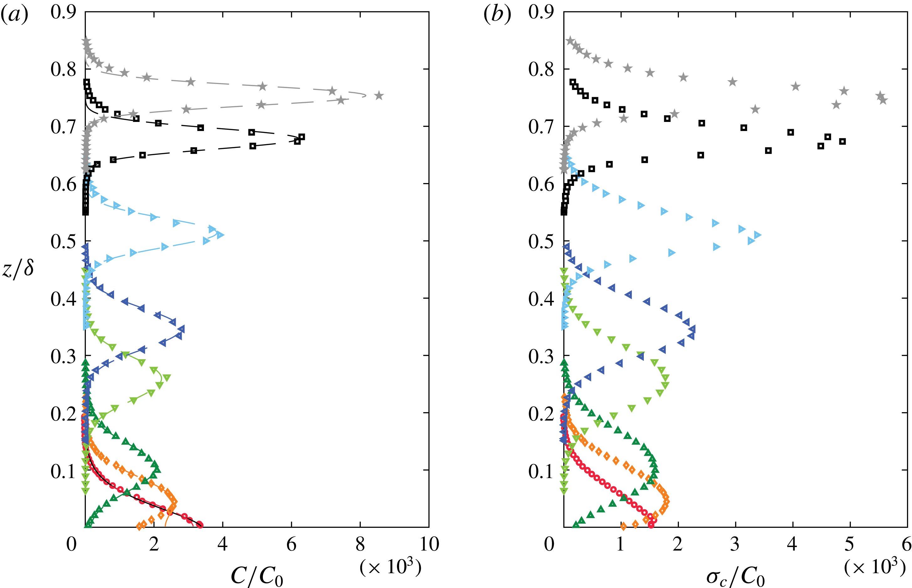
Profiles of normalised (a) mean and (b) root-mean-square of concentration as functions of
 $z/\unicode[STIX]{x1D6FF}$
for all source heights. Note that the initial concentration of tracer gas (
 $C_{0}=15\,000$
ppm) is used for normalisation. Symbols:
 $s_{z}/\unicode[STIX]{x1D6FF}=32/\unicode[STIX]{x1D6FF}^{+}$
(○),
 $350/\unicode[STIX]{x1D6FF}^{+}$
(♢),
 $0.1$
(▵),
 $0.25$
(▿),
 $0.33$
(◃),
 $0.5$
(▹),
 $0.67$
(▫),
 $\unicode[STIX]{x1D6FF}_{99}/\unicode[STIX]{x1D6FF}$
(
 $\star$
). Dashed lines in the mean concentration profiles represent the reflected Gaussian model, while the black solid line (only for
 $s_{z}/\unicode[STIX]{x1D6FF}=32/\unicode[STIX]{x1D6FF}^{+}$
) shows the exponential fit.

Results of mean,
 $C$
, and root-mean-square (r.m.s.),
 $\unicode[STIX]{x1D70E}_{c}$
, profiles of concentration for different source heights
 $s_{z}$
are plotted in figure 2(a,b), respectively. Note that the profiles are represented in the normalised form using the initial concentration of tracer gas,
 $C_{0}$
. The wall-normal distribution of
 $C$
can be modelled from the streamwise component of (1.1a
) by assuming an approximation for the vertical flux,
 $\overline{wc}$
, using the Reynolds’ analogy (of gradient diffusion theory) and neglecting viscous diffusion (e.g. Csanady Reference Csanady1973). One such model for an elevated source, which is widely adopted, is the reflected Gaussian distribution for
 $C$
(obtained as the solution of the diffusion equation with constant diffusivity and zero flux at the wall), and is given as (e.g. Csanady Reference Csanady1973; Fackrell & Robins Reference Fackrell and Robins1982)
 $$\begin{eqnarray}C(z)=A\left[\exp \left\{-B\left(\frac{z-s_{z}}{\unicode[STIX]{x1D6FF}_{C}}\right)^{2}\right\}+\exp \left\{-B\left(\frac{z+s_{z}}{\unicode[STIX]{x1D6FF}_{C}}\right)^{2}\right\}\right].\end{eqnarray}$$
Here,
 $A$
and
 $B$
are parameters obtained by fitting the data to the equation, and
 $\unicode[STIX]{x1D6FF}_{C}$
is the vertical plume half-width, which is defined as the vertical distance (with respect to the source height) where the local concentration is equal to half of the maximum mean concentration. The fit is shown in figure 2(a) by dashed lines, whereas
 $\unicode[STIX]{x1D6FF}_{C}$
for various source locations is plotted in figure 3. This fit represents the elevated sources well, except perhaps for the case of
 $s_{z}/\unicode[STIX]{x1D6FF}=350/\unicode[STIX]{x1D6FF}^{+}$
close to the ground, and definitely not the ground-level source.
For plumes emanating from a ground-level source and which exhibit self-preserving form of the vertical profile of mean concentration, the use gradient diffusion theory suggests a solution (Csanady Reference Csanady1973; Robins Reference Robins1978) as
 $$\begin{eqnarray}C(z)=C_{0}\left[\exp \left\{-b\left(\frac{z}{\unicode[STIX]{x1D6FF}_{C}}\right)^{\unicode[STIX]{x1D6FD}}\right\}\right],\end{eqnarray}$$
where
 $b=\ln (2)$
and
 $\unicode[STIX]{x1D6FD}$
is a parameter that depends on surface roughness (Csanady Reference Csanady1973; Hunt & Weber Reference Hunt and Weber1979). For instance, Fackrell & Robins (Reference Fackrell and Robins1982) obtained a value of 1.5 for
 $\unicode[STIX]{x1D6FD}$
in a rough-wall boundary layer while Robins (Reference Robins1978) reported a slightly higher value of
 $\unicode[STIX]{x1D6FD}=1.7$
in a rougher boundary layer. For our case, the ground-level source (
 $s_{z}/\unicode[STIX]{x1D6FF}=32/\unicode[STIX]{x1D6FF}^{+}\approx 0.0041$
) presented in figure 2(a) is well described by (3.2) with
 $\unicode[STIX]{x1D6FD}=1.5$
, which is close to the value reported by Fackrell & Robins (Reference Fackrell and Robins1982), and is indicated by a solid (black) line. For several engineering applications, the turbulent boundary layer mean velocity profile can be approximated with a power-law profile,
 $U=U_{\infty }(z/\unicode[STIX]{x1D6FF})^{\unicode[STIX]{x1D6FC}}$
, where
 $\unicode[STIX]{x1D6FC}$
is the power-law exponent, usually taken to be
 $1/7$
. In (3.2),
 $\unicode[STIX]{x1D6FD}$
can be shown to be equal to
 $(1+2\unicode[STIX]{x1D6FC})$
(Csanady Reference Csanady1973), which is not unreasonable.
Plume half-widths obtained from mean (
 $\unicode[STIX]{x1D6FF}_{C}$
, open symbols) and r.m.s. (
 $\unicode[STIX]{x1D6FF}_{\unicode[STIX]{x1D70E}}$
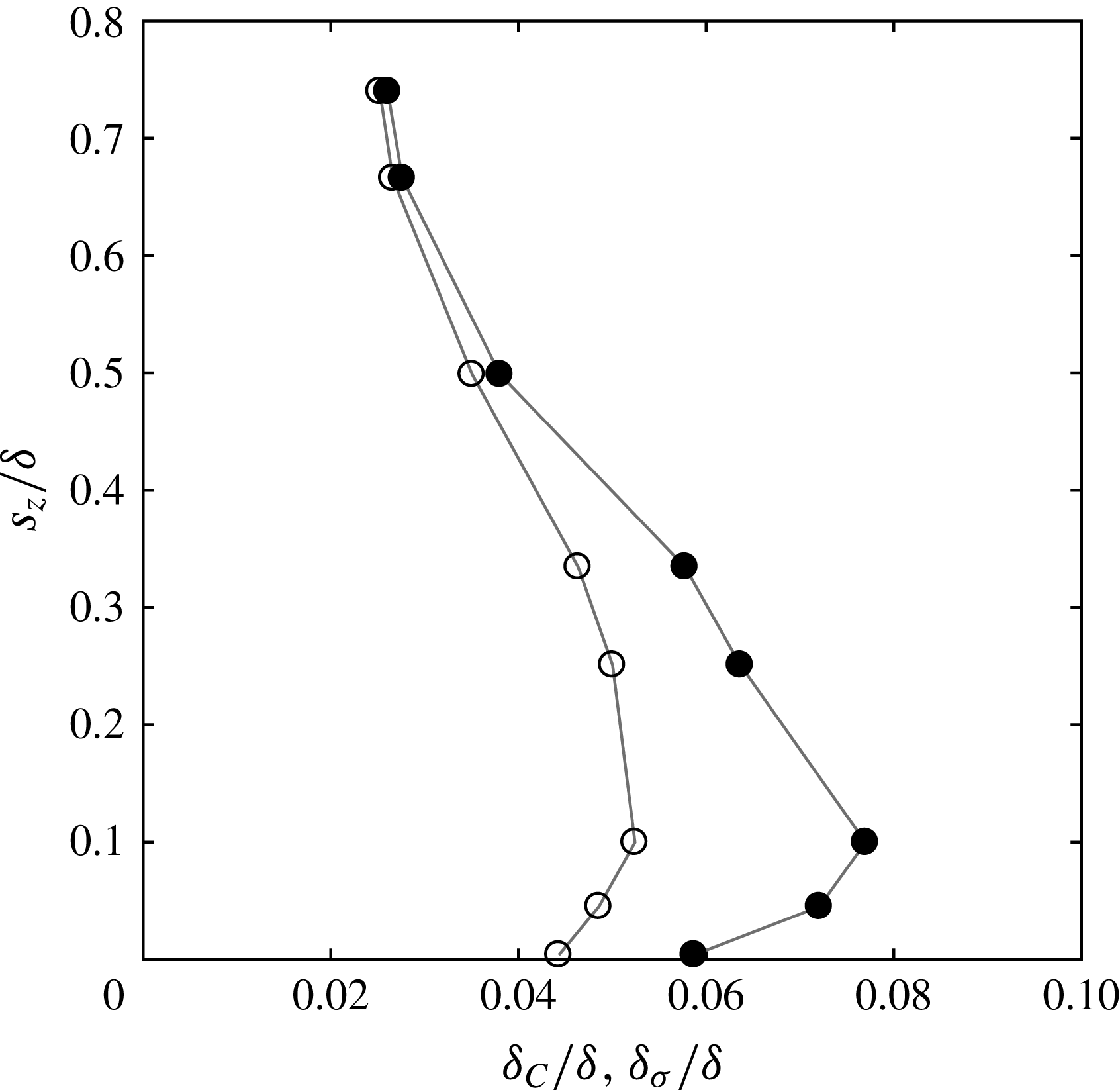
, filled symbols) profiles of concentration for different source heights.

We also present the wall-normal profiles of r.m.s.,
 $\unicode[STIX]{x1D70E}_{c}$
, of concentration for different source locations in figure 2(b), and the corresponding half-width
 $\unicode[STIX]{x1D6FF}_{\unicode[STIX]{x1D70E}}$
(determined from the location where
 $\unicode[STIX]{x1D70E}_{c}$
is half its peak centreline value) is shown in figure 3. The plume half-widths,
 $\unicode[STIX]{x1D6FF}_{C}$
and
 $\unicode[STIX]{x1D6FF}_{\unicode[STIX]{x1D70E}}$
, characterise the spatial extent where significant concentration events can be expected, albeit intermittently. In figure 3, it is observed that both
 $\unicode[STIX]{x1D6FF}_{C}$
and
 $\unicode[STIX]{x1D6FF}_{\unicode[STIX]{x1D70E}}$
increase up to
 $s_{z}/\unicode[STIX]{x1D6FF}=0.1$
, beyond which they decrease monotonically. Further,
 $\unicode[STIX]{x1D6FF}_{\unicode[STIX]{x1D70E}}$
is found to be larger than
 $\unicode[STIX]{x1D6FF}_{C}$
for source heights
 $s_{z}/\unicode[STIX]{x1D6FF}\leqslant 0.5$
, and there is negligible difference between the two at higher locations. In fact, we see that the width
 $\unicode[STIX]{x1D6FF}_{\unicode[STIX]{x1D70E}}$
corresponding to
 $\unicode[STIX]{x1D70E}_{C}$
is noticeably larger than
 $\unicode[STIX]{x1D6FF}_{C}$
in the log region, where high turbulence intensity and strong shear exist. Similar observations of
 $\unicode[STIX]{x1D6FF}_{\unicode[STIX]{x1D70E}}$
greater than
 $\unicode[STIX]{x1D6FF}_{C}$
are made by Vanderwel & Tavoularis (Reference Vanderwel and Tavoularis2014) in a uniformly sheared flow. This is also consistent with the well-accepted meandering plume model of Gifford (Reference Gifford1959), where an ‘instantaneous’ Gaussian plume, the width of which fluctuates randomly across the transverse direction, gives rise to an increased fluctuation width compared to the mean (see also Weil Reference Weil and Fernando2012).
In the present study, we have not investigated a model to fit the r.m.s. profiles, as such a model would require validation with varying streamwise source distance
 $s_{x}$
, which is beyond the scope of this paper. The aim here is to understand the role of velocity structures in scalar transport, and, as such, the data of
 $C$
and
 $\unicode[STIX]{x1D70E}_{c}$
presented here establish confidence in the measurements. Also note that, henceforth, the plume half-width refers to the
 $\unicode[STIX]{x1D6FF}_{\unicode[STIX]{x1D70E}}$
based on
 $\unicode[STIX]{x1D70E}_{c}$
profiles.
3.2 Autocorrelation and integral time scales
The autocorrelation function
 $R_{ii}(\boldsymbol{x},\unicode[STIX]{x0394}t)$
is defined as
 $$\begin{eqnarray}R_{ii}(\boldsymbol{x},\unicode[STIX]{x0394}t)=\overline{i(\boldsymbol{x},t)\,i(\boldsymbol{x},t+\unicode[STIX]{x0394}t)},\quad i=u,\,c.\end{eqnarray}$$
Note that the autocorrelation function will be different for varying source heights
 $s_{z}$
. For the wall-normal profile measurements considered here, the integral time scales of velocity,
 $\unicode[STIX]{x1D70F}_{u}$
, and concentration,
 $\unicode[STIX]{x1D70F}_{c}$
, are calculated from the autocorrelation function as
 $$\begin{eqnarray}\unicode[STIX]{x1D70F}_{i}(z)=\int _{0}^{\infty }\frac{R_{ii}(z,t^{\prime })}{[\unicode[STIX]{x1D70E}_{i}(z)]^{2}}\,\text{d}t^{\prime },\end{eqnarray}$$
with
 $\unicode[STIX]{x1D70E}_{i}^{2}$
as the variance of the fluctuating quantity.
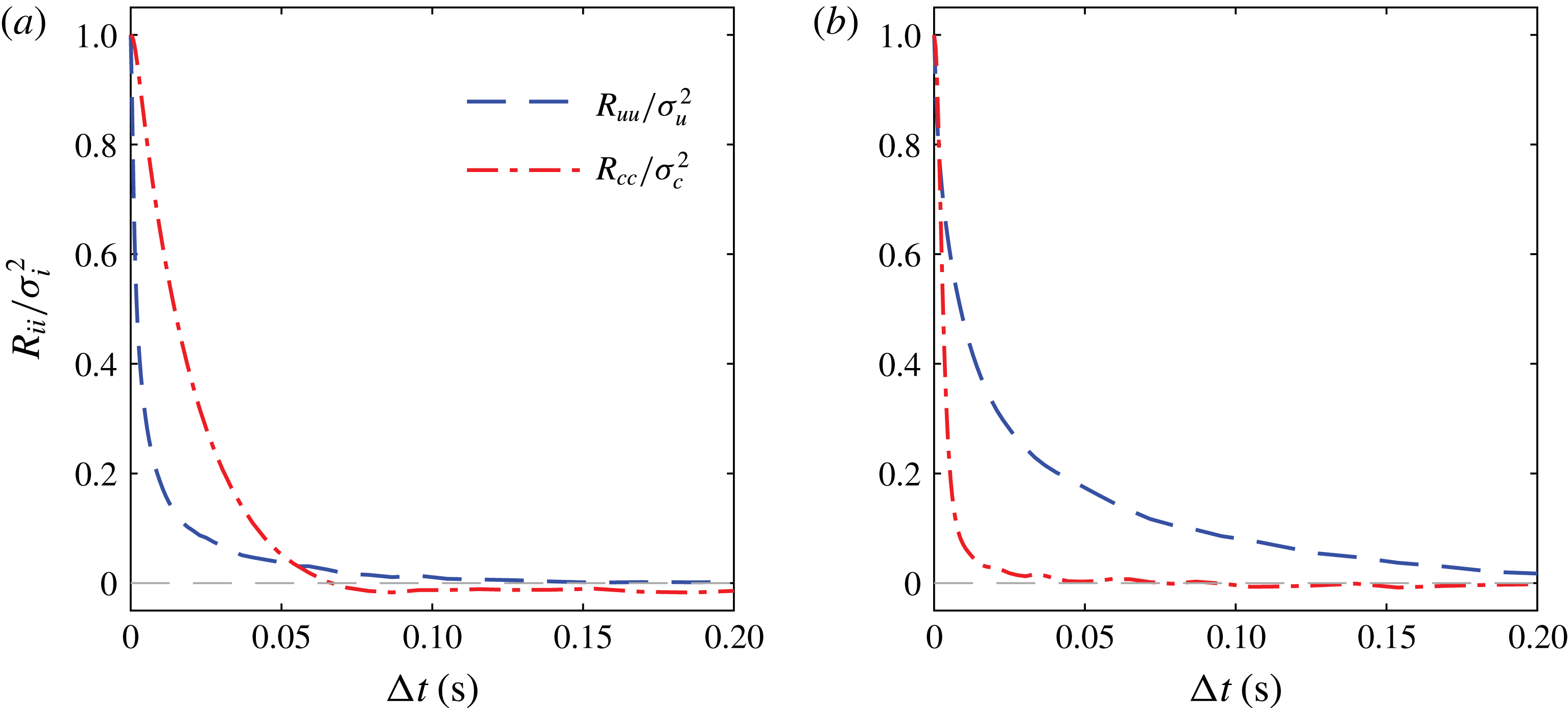
Comparison of
 $R_{ii}/\unicode[STIX]{x1D70E}_{i}^{2}~(i=u,c)$
at the centreline of the plume for (a)
 $s_{z}/\unicode[STIX]{x1D6FF}=32/\unicode[STIX]{x1D6FF}^{+}$
, the ground-level source, where
 $\unicode[STIX]{x1D70F}_{u}~(0.008~\text{s})<\unicode[STIX]{x1D70F}_{c}~(0.017~\text{s})$
, and (b)
 $s_{z}/\unicode[STIX]{x1D6FF}=0.1$
, the log-region source, where
 $\unicode[STIX]{x1D70F}_{u}~(0.028~\text{s})>\unicode[STIX]{x1D70F}_{c}~(0.004~\text{s})$
. Note that
 $\unicode[STIX]{x1D70F}_{c}$
is calculated by integrating
 $R_{cc}/\unicode[STIX]{x1D70E}_{c}^{2}$
up to its first zero crossing, while
 $\unicode[STIX]{x1D70F}_{u}$
is obtained by integrating
 $R_{uu}/\unicode[STIX]{x1D70E}_{u}^{2}$
in the interval
 $0\leqslant \unicode[STIX]{x0394}t\leqslant 1.2~\text{s}$
, which is equivalent to a streamwise length of 40
 $\unicode[STIX]{x1D6FF}$
.

The integral time scales
 $\unicode[STIX]{x1D70F}_{u}$
and
 $\unicode[STIX]{x1D70F}_{c}$
indicate the average duration of a coherent velocity structure or a scalar/concentration region passing through the measurement location. The integral time scale for concentration,
 $\unicode[STIX]{x1D70F}_{c}$
, is relevant to estimates of ‘exposure times’, a measure of the time duration over which concentration levels exceed a certain threshold. It is found that
 $\unicode[STIX]{x1D70F}_{c}$
is higher than
 $\unicode[STIX]{x1D70F}_{u}$
for a ground-level source as inferred from figure 4(a), showing
 $R_{cc}$
and
 $R_{uu}$
for
 $s_{z}/\unicode[STIX]{x1D6FF}=32/\unicode[STIX]{x1D6FF}^{+}$
. This may be attributed to two factors. First, intense small-scale activity of velocity fluctuations in the near-wall region leads to a faster decline of autocorrelation of
 $u$
in time, resulting in a smaller magnitude of
 $\unicode[STIX]{x1D70F}_{u}$
. Second, concentration tends to persist for longer time near the wall since the streamwise mean velocity is relatively low, and, combined with the fact that concentration flux is zero at the wall, longer correlations and higher integral time scales are measured. On the other hand, for all elevated sources,
 $\unicode[STIX]{x1D70F}_{c}$
is typically smaller than
 $\unicode[STIX]{x1D70F}_{u}$
, as illustrated in figure 4(b) for a source in the logarithmic region, with
 $R_{uu}$
and
 $R_{cc}$
again measured on the centreline of the plume. This in turn implies that the length scales associated with concentration are smaller than the length scale of turbulent motions. This is consistent with the arguments put forth by Tennekes & Lumley (Reference Tennekes and Lumley1972) (see also Duplat & Villermaux Reference Duplat and Villermaux2008), i.e. the turbulence will mix the scalar at the smallest scales of velocity, resulting in a short correlation time, whereas velocity correlation times (at least in shear flows) are dominated by large coherent structures leading to a longer time scale compared to the scalar.
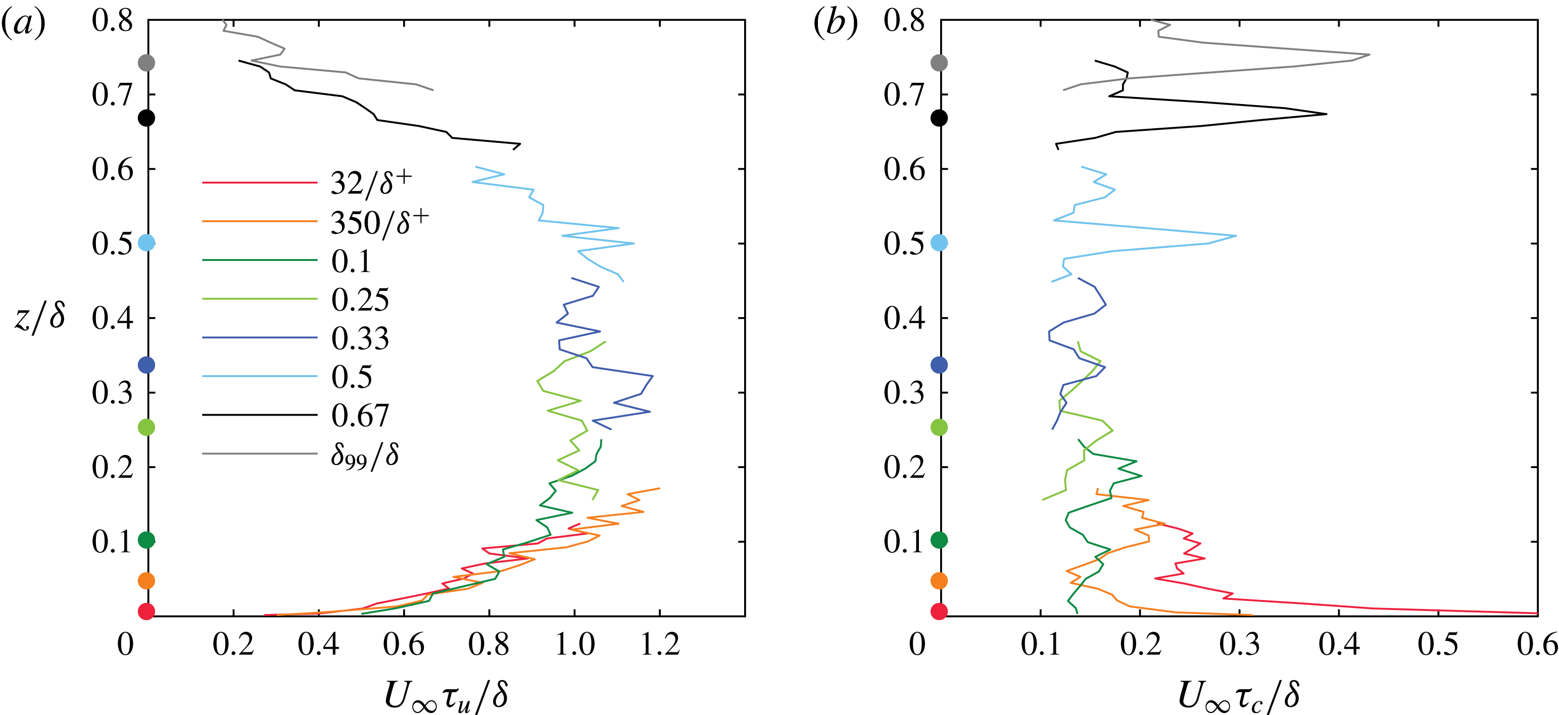
Comparison of integral time scales of (a) velocity and (b) concentration fluctuations for different source heights indicated by coloured dots on the ordinate axis.

As an aside, we note that, in the Eulerian frame of reference, the integral length scale for velocity fluctuations in a fully developed turbulent flow can be computed from the integral time scale by invoking Taylor’s frozen turbulence hypothesis and assuming local mean velocity as the convection velocity. This has been shown to be approximately valid (Dennis & Nickels Reference Dennis and Nickels2008; Del Álamo & Jiménez Reference Del Álamo and Jiménez2009) for velocity structures in wall-bounded flows. This hypothesis, however, is not applicable to a scalar concentration field that is rapidly changing downstream of a point source. Hence, the discussion here is limited to the integral time (rather than length) scales of
 $u$
and
 $c$
that are unambiguously calculated from single-point measurements.
Figure 5(a,b) shows the integral time scales of velocity and concentration for different source heights in the boundary layer. Note that there are more than 200 measurement points and the scatter in the values of
 $\unicode[STIX]{x1D70F}_{u}$
is acceptable, with a clear trend in
 $\unicode[STIX]{x1D70F}_{u}$
as a function of
 $z/\unicode[STIX]{x1D6FF}$
. It is seen that
 $\unicode[STIX]{x1D70F}_{u}$
increases up to
 $z/\unicode[STIX]{x1D6FF}\approx 0.2$
, approximately remains constant between
 $0.2\lesssim z/\unicode[STIX]{x1D6FF}\lesssim 0.5$
and then decreases up to the edge of the boundary layer. The increase of
 $\unicode[STIX]{x1D70F}_{u}$
adjacent to the wall is expected as the large-scale motions become prominent in the inner region with increasing wall-normal height. In the region
 $z/\unicode[STIX]{x1D6FF}\gtrsim 0.5$
, there is a decreasing trend of
 $\unicode[STIX]{x1D70F}_{u}$
due to increasing external intermittency, i.e. length scales associated with turbulent motions will be confined within regions of turbulent zones that are preceded and followed by non-turbulent regions. Since the relative population of turbulent zones decreases with increasing distance from the wall,
 $\unicode[STIX]{x1D70F}_{u}$
decreases towards the edge of the boundary layer. Note that
 $\unicode[STIX]{x1D70F}_{u}$
was also computed with data from a single hotwire (without any PID and the gas discharge tube), and the results are not different from what is presented in figure 5(a), although with less scatter.
Note that the magnitude of
 $\unicode[STIX]{x1D70F}_{u}$
is scaled with
 $\unicode[STIX]{x1D6FF}/U_{\infty }$
, and the values are around unity, which suggests that
 $\unicode[STIX]{x1D70F}_{u}$
is governed by the large-scale outer motions. Using a simplistic approximation of the integral time scales in shear flows to be of the order of the inverse of the mean shear, or
 $1/S\equiv 1/(\text{d}U/\text{d}z)$
, the usual logarithmic mean velocity profile approximation (
 $U^{+}=(1/\unicode[STIX]{x1D705})\ln (z^{+})+A$
) leads to a shear time scale of
 $(1/S)U_{\infty }/\unicode[STIX]{x1D6FF}=U_{\infty }^{+}\unicode[STIX]{x1D705}(z/\unicode[STIX]{x1D6FF})$
(where
 $\unicode[STIX]{x1D705}=0.384$
is the von Kármán constant), which is equal to
 $1.07$
for
 $z/\unicode[STIX]{x1D6FF}=0.1$
. Note that this time scale turns out to be
 $0.97$
if we approximate the velocity profile with a power law (
 $U=U_{\infty }(z/\unicode[STIX]{x1D6FF})^{\unicode[STIX]{x1D6FC}}$
) with
 $\unicode[STIX]{x1D6FC}=1/7$
. These estimates are in the range of what we observe in figure 5(a), and as such valid in the region
 $0.1\lesssim z/\unicode[STIX]{x1D6FF}\lesssim 0.6$
.
The variation of the integral time scale of concentration
 $\unicode[STIX]{x1D70F}_{c}$
is shown in figure 5(b), and is quite different from
 $\unicode[STIX]{x1D70F}_{u}$
. The collective trend of all data in figure 5(b) indicates that
 $\unicode[STIX]{x1D70F}_{c}$
is high close to the wall and near the edge of the boundary layer, whereas it does not vary significantly in the region
 $0.1<z/\unicode[STIX]{x1D6FF}<0.5$
. These observations are consistent with those of Fackrell & Robins (Reference Fackrell and Robins1982) for one ground-level and one elevated source. It is clear that
 $\unicode[STIX]{x1D70F}_{c}$
is influenced by background turbulence and the mean shear. Particularly, it should be noted that
 $\unicode[STIX]{x1D70F}_{c}$
measured closer to the wall is significantly higher when the source is also in the vicinity of the wall. This behaviour could be due to small-scale turbulent motions close to the wall being effective in mixing and attenuating small-scale concentration fluctuations such that large-scale concentration patches remain, and they are associated with plume meandering. Comparing figures 5(a) and 5(b) shows that
 $\unicode[STIX]{x1D70F}_{u}$
and
 $\unicode[STIX]{x1D70F}_{c}$
have opposing overall trends, i.e. higher
 $\unicode[STIX]{x1D70F}_{u}$
corresponds to relatively lower
 $\unicode[STIX]{x1D70F}_{c}$
and vice versa. This behaviour is again consistent with small velocity scales leading to better mixing and longer correlated scalar fields.
To put a perspective on the magnitude of
 $\unicode[STIX]{x1D70F}_{c}$
in figure 5(b), it is worth considering the time scales associated with the smallest turbulent motions, i.e. the Kolmogorov time scale
 $\unicode[STIX]{x1D70F}_{\unicode[STIX]{x1D708}}=\sqrt{\unicode[STIX]{x1D708}/\unicode[STIX]{x1D700}}$
, where
 $\unicode[STIX]{x1D700}$
is the dissipation rate of kinetic energy and
 $\unicode[STIX]{x1D70F}_{\unicode[STIX]{x1D708}}$
is sometimes considered to be the time of mixing or homogenisation (Tennekes & Lumley Reference Tennekes and Lumley1972). Estimating
 $\unicode[STIX]{x1D700}\approx U_{\unicode[STIX]{x1D70F}}^{2}\,\text{d}U/\text{d}z$
, where
 $\text{d}U/\text{d}z$
is evaluated by assuming a logarithmic profile for mean velocity (
 $U^{+}=(1/\unicode[STIX]{x1D705})\ln z^{+}+A$
), leads to
 $\unicode[STIX]{x1D70F}_{\unicode[STIX]{x1D708}}U_{\infty }/\unicode[STIX]{x1D6FF}\approx U_{\infty }^{+}\sqrt{\unicode[STIX]{x1D705}z^{+}}/\unicode[STIX]{x1D6FF}^{+}$
. For
 $z/\unicode[STIX]{x1D6FF}=0.1$
, we obtain
 $\unicode[STIX]{x1D70F}_{\unicode[STIX]{x1D708}}U_{\infty }/\unicode[STIX]{x1D6FF}\approx 0.062$
(and
 $0.060$
if we approximate
 $U$
with a power-law profile). As such,
 $\unicode[STIX]{x1D70F}_{\unicode[STIX]{x1D708}}U_{\infty }/\unicode[STIX]{x1D6FF}$
is observed to be smaller than the typical
 $\unicode[STIX]{x1D70F}_{c}U_{\infty }/\unicode[STIX]{x1D6FF}$
values reported in figure 5(b). This is perhaps not surprising considering that, in a turbulent boundary layer, the dynamics are governed by the velocity fluctuations due to vortical motions, which are of the order of the Taylor microscale
 $\unicode[STIX]{x1D706}$
(e.g. Chauhan, Philip & Marusic Reference Chauhan, Philip and Marusic2014a
; de Silva et al.
Reference de Silva, Philip, Hutchins and Marusic2017). If we consider the time scale based on
 $\unicode[STIX]{x1D706}$
and the fluctuating velocity (
 $\unicode[STIX]{x1D70E}_{u}$
), i.e.
 $\unicode[STIX]{x1D70F}_{\unicode[STIX]{x1D706}}=\unicode[STIX]{x1D706}/\unicode[STIX]{x1D70E}_{u}$
, and estimating
 $\unicode[STIX]{x1D706}$
from
 $\unicode[STIX]{x1D700}=15\unicode[STIX]{x1D708}(\unicode[STIX]{x1D70E}_{u}/\unicode[STIX]{x1D706})^{2}$
, this leads to
 $\unicode[STIX]{x1D70F}_{\unicode[STIX]{x1D706}}U_{\infty }/\unicode[STIX]{x1D6FF}\approx U_{\infty }^{+}\sqrt{15\unicode[STIX]{x1D705}z^{+}}/\unicode[STIX]{x1D6FF}^{+}$
. Then, for
 $z/\unicode[STIX]{x1D6FF}=0.1$
, we obtain
 $\unicode[STIX]{x1D70F}_{\unicode[STIX]{x1D706}}U_{\infty }/\unicode[STIX]{x1D6FF}\approx 0.24$
. This estimate of
 $\unicode[STIX]{x1D70F}_{\unicode[STIX]{x1D706}}$
is closer to the values of
 $\unicode[STIX]{x1D70F}_{c}$
reported in figure 5(b), and shows that the time scale of mixing is probably governed by velocity fluctuations.
Further, from figure 5, it is seen that the integral time scale of velocity fluctuations is an order of magnitude higher than the integral time scale of concentration, i.e.
 $\unicode[STIX]{x1D70F}_{u}/\unicode[STIX]{x1D70F}_{c}=O(10)$
. This observation and its implication are discussed later in § 3.3 along with a discussion on spectra.
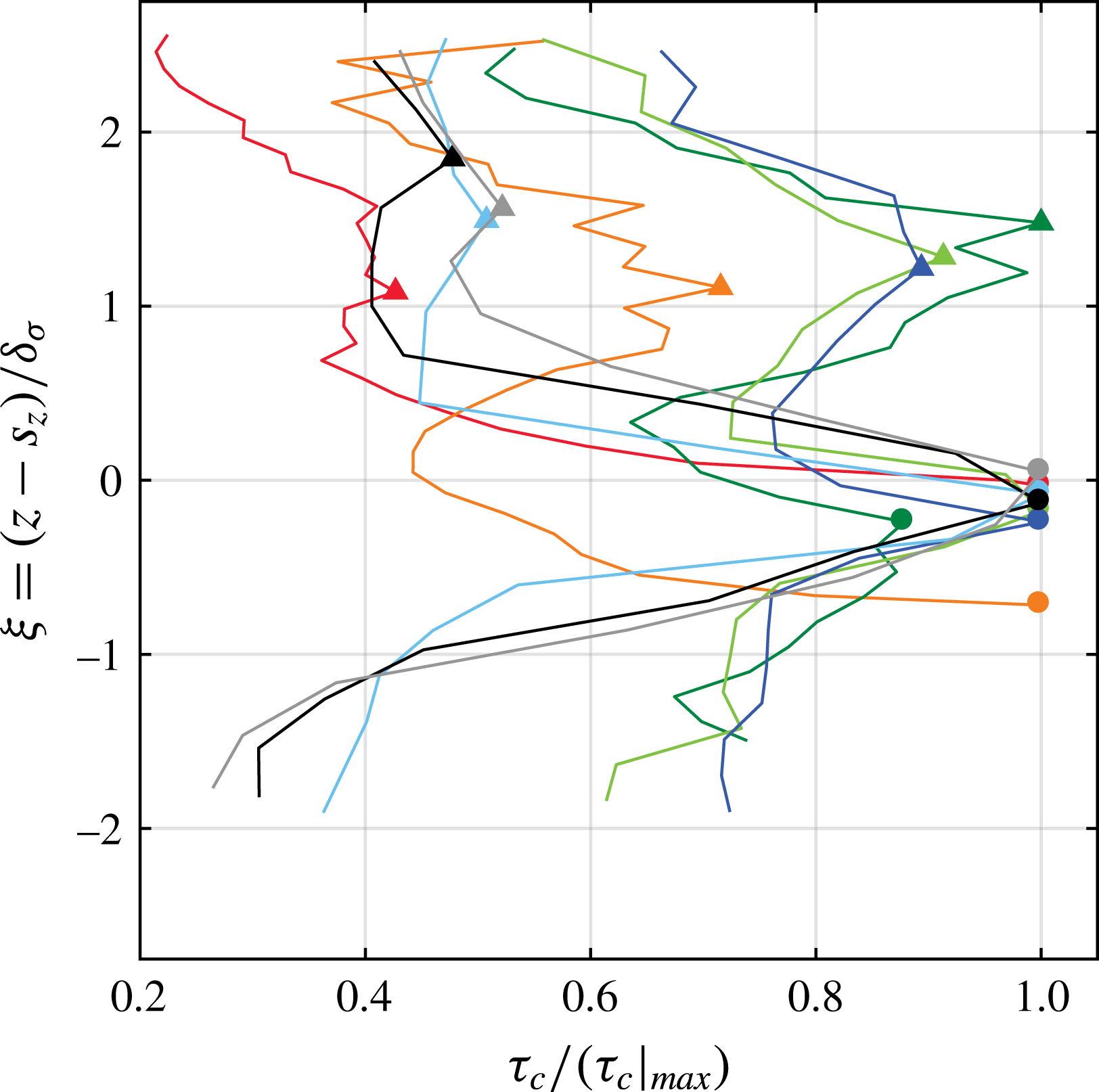
Closer examination of figure 5(b) indicates that two prominent peaks are present in
 $\unicode[STIX]{x1D70F}_{c}$
profiles; the lower peak is closer to the plume centreline while the upper peak is approximately at a distance of
 $\unicode[STIX]{x1D6FF}_{\unicode[STIX]{x1D70E}}$
above the plume centreline. This feature is better illustrated in figure 6, where normalised integral time scale
 $\unicode[STIX]{x1D70F}_{c}/(\unicode[STIX]{x1D70F}_{c}|_{max})$
values are plotted against
 $\unicode[STIX]{x1D709}=(z-s_{z})/\unicode[STIX]{x1D6FF}_{\unicode[STIX]{x1D70E}}$
. In this coordinate system,
 $\unicode[STIX]{x1D709}=1$
corresponds to one half-width (based on
 $\unicode[STIX]{x1D70E}_{c}$
) above the centreline of a plume. The peak in
 $\unicode[STIX]{x1D70F}_{c}$
near the centreline is most prominent for source heights
 $s_{z}/\unicode[STIX]{x1D6FF}=32/\unicode[STIX]{x1D6FF}^{+},~350/\unicode[STIX]{x1D6FF}^{+},~0.5,~0.67$
and
 $\unicode[STIX]{x1D6FF}_{99}/\unicode[STIX]{x1D6FF}$
, whereas the second peak (near
 $\unicode[STIX]{x1D709}=1$
) becomes relatively less prominent as
 $s_{z}$
increases. However, for sources located in the fully turbulent regions,
 $s_{z}/\unicode[STIX]{x1D6FF}=0.1$
, 0.25 and 0.33, the two peaks are equivalent in magnitude. For sources located closer to the wall, i.e.
 $s_{z}/\unicode[STIX]{x1D6FF}\leqslant 0.1$
, it is interesting to note that the peak in
 $\unicode[STIX]{x1D70F}_{c}$
occurs below the centreline. This is probably because meandering of the plume below the centreline is restricted due to the presence of the wall. In addition, the convection velocity is relatively small at these locations, which results in a longer time for the scalar to be advected away, leading to higher magnitude of
 $\unicode[STIX]{x1D70F}_{c}$
at locations below the plume centreline.
Normalised integral time scale of
 $c$
(
 $\unicode[STIX]{x1D70F}_{c}/(\unicode[STIX]{x1D70F}_{c}|_{max})$
) for all source heights as a function of
 $\unicode[STIX]{x1D709}=(z-s_{z})/\unicode[STIX]{x1D6FF}_{\unicode[STIX]{x1D70E}}$
. The peak in
 $\unicode[STIX]{x1D70F}_{c}$
closer to
 $\unicode[STIX]{x1D709}=0$
is shown by solid circles, while the other peak is represented by solid triangles. Line colours as in figure 5.

A similar result of a double peak in
 $\unicode[STIX]{x1D70F}_{c}$
was reported by Yee & Biltoft (Reference Yee and Biltoft2004) in their full-scale atmospheric measurements of tracer gas dispersed through a large array of building-like obstacles. However, no explanation was provided for the existence of the double peak. It should be noted that the present discussion is based on
 $\unicode[STIX]{x1D70F}_{c}$
computed in an Eulerian frame of reference. Unfortunately, it is extremely difficult to make direct measurements of Lagrangian time scales. Typically, they are inferred from Eulerian measurements (see McComb Reference McComb1990, for details) and it is usually hypothesised that Lagrangian and Eulerian correlation functions have similar shapes but different scales. However, we are unable to conclude whether or not a double peak exists in Lagrangian time scales.
It is clear from figure 6 that
 $\unicode[STIX]{x1D70F}_{c}$
has an asymmetric behaviour about the plume centreline. This asymmetry is a result of the variation in convection velocities as one moves across the boundary layer. Further, the integral time scales are higher away from the source height due to the (vertical) meandering or oscillating nature of the plume whereby it spends more time at the extreme ends. We shall elaborate on this phenomenon in § 5.1 via a phenomenological model for velocity–concentration organisation.
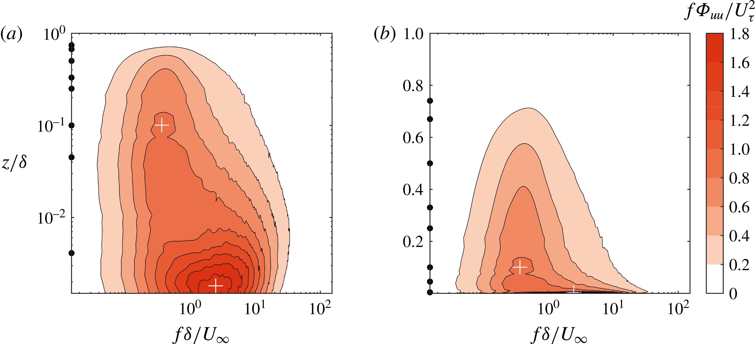
Contour map of pre-multiplied energy spectra of velocity fluctuations: (a) log–log and (b) log–linear scaling for abscissa and ordinate, respectively. Locations of inner and outer peaks in the energy spectra are indicated by ‘+’.

Contour maps of pre-multiplied spectra (
 $f\unicode[STIX]{x1D6F7}_{cc}/\unicode[STIX]{x1D70E}_{c,\,max}^{2}$
) of concentration fluctuations for different source heights. Here,
 $\unicode[STIX]{x1D70E}_{c,\,max}^{2}$
represents the maxima in variance of concentration across the plume. Contours of
 $f\unicode[STIX]{x1D6F7}_{uu}/U_{\unicode[STIX]{x1D70F}}^{2}$
are shown in red. The red dashed lines represent the locus of local maxima of energy spectra of
 $u$
at different
 $z$
-locations in the boundary layer. The horizontal black dot-dashed line in each panel indicates the source location.

3.3 Pre-multiplied energy spectra
We will consider the contribution of different frequencies to the energy spectra of
 $u$
and
 $c$
in this section. The (one-sided) spectral density
 $\unicode[STIX]{x1D6F7}_{ii}$
and the autocorrelation function
 $R_{ii}$
are Fourier-transform pairs, and hence
 $\unicode[STIX]{x1D6F7}_{ii}$
is defined as
 $$\begin{eqnarray}\frac{1}{2}\unicode[STIX]{x1D6F7}_{ii}(f)=\frac{1}{2\unicode[STIX]{x03C0}}\int _{-\infty }^{\infty }R_{ii}(t)\text{e}^{-\text{j}\,ft}\,\text{d}t,\quad i=u,\,c,\end{eqnarray}$$
where
 $\text{j}$
represents the imaginary unit, and
 $t$
and
 $f$
are the corresponding time and frequency pairs. In order to facilitate visual integration of energy over a certain frequency range, spectra are presented in the pre-multiplied form as
 $f\unicode[STIX]{x1D6F7}_{ii}$
such that the variance
 $\unicode[STIX]{x1D70E}_{i}^{2}$
of a signal
 $i$
can be written as
 $$\begin{eqnarray}\unicode[STIX]{x1D70E}_{i}^{2}=\int _{0}^{\infty }\unicode[STIX]{x1D6F7}_{ii}(f)\,\text{d}f=\int _{0}^{\infty }f\unicode[STIX]{x1D6F7}_{ii}\,\text{d}\ln f.\end{eqnarray}$$
We first examine the pre-multiplied energy spectrogram of streamwise velocity (
 $f\unicode[STIX]{x1D6F7}_{uu}$
) in figure 7 as functions of normalised frequency and wall-normal distance. Note that figure 7(a) utilises a log–log scale whereas 7(b) is with a linear–log scale. The well-known ‘double peak’ in the spectrogram is also observed (see e.g. Hutchins & Marusic Reference Hutchins and Marusic2007a
), and indicated by white ‘+’ mark in the figure. The peak at higher frequency is associated with small-scale fluctuations and scales with viscous units
 $U_{\unicode[STIX]{x1D70F}}^{2}/\unicode[STIX]{x1D708}$
; whereas the one at lower frequency is a consequence of large-scale motions in the logarithmic region and above, and scales with
 $U_{\infty }/\unicode[STIX]{x1D6FF}$
. As mentioned earlier, one cannot apply Taylor’s hypothesis to the concentration signal and thus we are restricted to examine
 $\unicode[STIX]{x1D6F7}_{cc}$
as a function of frequency. This will enable us to make a one-to-one comparison between
 $\unicode[STIX]{x1D6F7}_{cc}$
and
 $\unicode[STIX]{x1D6F7}_{uu}$
.
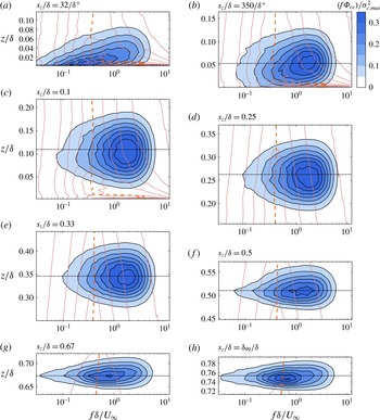
Figure 8 shows the comparison of the pre-multiplied energy spectrogram of concentration fluctuations (
 $f\unicode[STIX]{x1D6F7}_{cc}$
) as filled contour maps for different source heights. In each panel, contours of
 $f\unicode[STIX]{x1D6F7}_{uu}/U_{\unicode[STIX]{x1D70F}}^{2}$
(the same as in figure 7
b) are overlaid as line plots. Also note that the ordinate scale of each panel is proportional although their vertical limits are different, providing a visual approximation of plume spread.
The most evident feature in figure 8 is that peaks in energy of
 $u$
(indicated by thick red dashed lines) at different heights are at a lower frequency compared to peak frequencies of concentration spectra. Peaks in concentration spectra occur at frequency
 $f\sim 50{-}80$
Hz compared to
 $f\sim 10{-}15$
Hz for velocity spectra. Except for the source at ground level, the frequency at which the most energetic fluctuations in
 $c$
occur decreases as the source location moves higher in the boundary layer. This behaviour is consistent with previous observation that the integral time scales of concentration fluctuations (
 $\unicode[STIX]{x1D70F}_{c}$
) are an order of magnitude smaller than those of velocity fluctuations (
 $\unicode[STIX]{x1D70F}_{u}$
). The ground-level source (
 $s_{z}/\unicode[STIX]{x1D6FF}=32/\unicode[STIX]{x1D6FF}^{+}$
), however, is an exception, where the peak frequencies for
 $c$
spectra increase with increasing
 $z$
. This behaviour reflects the steep decrease in
 $\unicode[STIX]{x1D70F}_{c}$
observed near the wall in figure 5(b).
The lower peak frequency in the velocity spectra corresponds to a streamwise wavelength (by assuming local mean velocity as the convection velocity),
 $\unicode[STIX]{x1D706}_{x}\sim (6{-}10)\unicode[STIX]{x1D6FF}$
consistent with the sizes of large-scale structures reported in the literature. Overall, figure 8 suggests that large-scale velocity structures play only an indirect role, if any, on the structure of concentration in a boundary layer, where the concentration variation itself is at smaller spatial scale. This is expected, since in § 3.2 it is seen that typical time scales for concentration mixing are similar to those of small-scale velocity features, and hence have higher frequencies. A clearer understanding of the interaction between large-scale velocity and concentration is obtained by examining scalar flux (
 $\overline{uc}$
) in the next section.
4 Organisation of velocity and concentration in the flow
Here we shall utilise the simultaneously measured velocity and scalar concentration to discuss velocity–scalar fluxes for different source heights, and their cross-spectral and phase relations.
4.1 Streamwise scalar flux
The gradient of streamwise scalar flux
 $\overline{uc}$
appears in the streamwise component of (1.1a
) and is pertinent to downstream evolution of the plume. In practice,
 $\overline{uc}$
is neglected for being small in comparison to the mean transport (
 $\overline{UC}$
) in (1.1a
). To verify this, the streamwise turbulent flux
 $\overline{uc}$
is compared against
 $\overline{UC}$
across the plume released from a point source at
 $s_{z}/\unicode[STIX]{x1D6FF}=0.1$
. It is found that
 $\overline{uc}$
is less than 4 % of
 $\overline{UC}$
, justifying the common approach of neglecting
 $\overline{uc}$
in (1.1a
) for predicting
 $C$
. However, the gradients of transverse (
 $\overline{vc}$
) and vertical (
 $\overline{wc}$
) fluxes in the respective directions are significant, as they play a key role in spreading the plume. Further experiments aimed at characterising the gradients of these fluxes in the respective directions will be of great value.
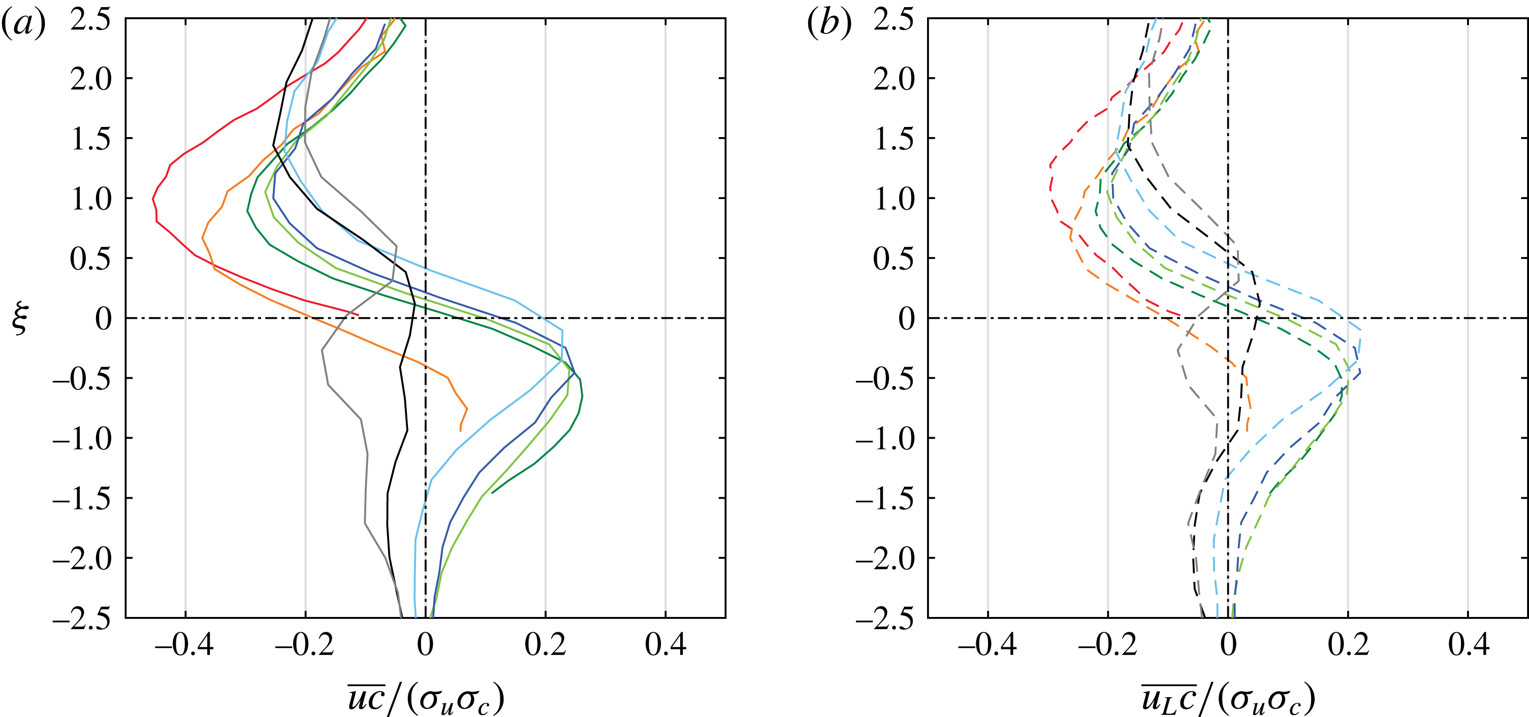
The distribution of
 $\overline{uc}$
as a function of wall-normal distance is shown in figure 9(a) for all source heights. The results for
 $\overline{uc}$
are presented using the local ordinate
 $\unicode[STIX]{x1D709}=(z-s_{z})/\unicode[STIX]{x1D6FF}_{\unicode[STIX]{x1D70E}}$
in order to examine the characteristic behaviour of
 $\overline{uc}$
in the vicinity of the plume centreline. For all source heights,
 $\overline{uc}$
is negative above the plume centreline (
 $\unicode[STIX]{x1D709}=0$
), while for
 $s_{z}/\unicode[STIX]{x1D6FF}\leqslant 0.5$
,
 $\overline{uc}$
tends to be positive below
 $\unicode[STIX]{x1D709}=0$
. Differing in trend from others, in the intermittent region, i.e.
 $s_{z}/\unicode[STIX]{x1D6FF}=0.67$
and
 $\unicode[STIX]{x1D6FF}_{99}/\unicode[STIX]{x1D6FF}$
,
 $\overline{uc}$
is negative below the plume centreline.
In a laminar flow, the plume will spread only by the action of diffusion, whereas in a turbulent flow, a passive scalar will be carried in the lateral and vertical directions by
 $v$
and
 $w$
fluctuations, respectively. In the wall-normal direction, positive
 $w$
fluctuations carry the scalar above the centreline and negative
 $w$
fluctuations below the centreline. Since the Reynolds stress
 $\overline{uw}$
is negative throughout the boundary layer, negative
 $u$
fluctuations are correlated with positive
 $w$
fluctuations that are associated with upwards scalar transport, resulting in negative
 $\overline{uc}$
above the centreline. Similarly, positive
 $u$
fluctuations are correlated with negative
 $w$
fluctuations that are responsible for downwards scalar transport, leading to positive
 $\overline{uc}$
below the plume centreline. Thus, low-speed motions are associated with negative scalar flux above the plume centreline, and high-speed motions are associated with positive scalar flux below the centreline. This behaviour is supported by joint probability density functions discussed in § 5.1 and forms the basis of organisation of concentration patches in the flow relative to high- and low-speed velocity features.
Negative
 $\overline{uc}$
for
 $s_{z}/\unicode[STIX]{x1D6FF}=0.67$
and
 $\unicode[STIX]{x1D6FF}_{99}/\unicode[STIX]{x1D6FF}$
can be explained by considering the influence of external intermittency in the calculation of statistics. At
 $s_{z}/\unicode[STIX]{x1D6FF}=0.67$
the
 $\tilde{U}$
signal has approximately
 $50\,\%$
of non-turbulent region and even higher fraction for the source at
 $\unicode[STIX]{x1D6FF}_{99}/\unicode[STIX]{x1D6FF}$
. In the non-turbulent region, the velocity is close to
 $U_{\infty }$
(typically approximately
 $0.95U_{\infty }$
; see Townsend (Reference Townsend1976) and also Chauhan et al. (Reference Chauhan, Philip, de Silva, Hutchins and Marusic2014b
)). Therefore, the fluctuating streamwise velocity
 $u=\tilde{U}-U$
is typically negative in the turbulent region due to biased mean, resulting in a negative
 $\overline{uc}$
. It is also found from a preliminary calculation that, at the centreline for
 $s_{z}/\unicode[STIX]{x1D6FF}=0.67$
, the turbulent zones in the signal contribute approximately
 $85\,\%$
of
 $\overline{uc}$
.
Comparison of (a) streamwise concentration flux normalised by the r.m.s. of
 $u$
and
 $c$
for different source heights, and (b) the contribution of large scales of velocity to scalar flux. Line colours as in figure 5.

In § 3.3, the energy spectra of
 $u$
and
 $c$
revealed that the dominant frequency for velocity was smaller (indicating large scales) than that for the scalar. In order to understand the contribution of low-frequency velocity structures to the streamwise scalar flux (
 $\overline{uc}$
), the instantaneous velocity is decomposed into large and small scales using a cut-off filter corresponding to a wavelength of
 $1\unicode[STIX]{x1D6FF}$
such that
 $u=u_{L}+u_{S}$
, where
 $u_{L}$
and
 $u_{S}$
are the large- and small-scale velocity components, respectively. The choice of
 $1\unicode[STIX]{x1D6FF}$
as the filter cut-off is adopted from previous studies (Hutchins & Marusic Reference Hutchins and Marusic2007b
; Mathis, Hutchins & Marusic Reference Mathis, Hutchins and Marusic2009) in a smooth-wall zero-pressure-gradient turbulent boundary layer. The resulting large-scale concentration flux
 $\overline{u_{L}c}$
is plotted in figure 9(b), noting that
 $\overline{uc}=\overline{u_{L}c}+\overline{u_{S}c}$
. It is clear that
 $\overline{u_{L}c}$
contributes significantly to the magnitude of
 $\overline{uc}$
, a conclusion that could not be drawn from spectra alone. The strong
 $\overline{u_{L}c}$
correlation implies that, although high-concentration regions in the flow occur at smaller spatial scales, they are effectively transported by large-scale motions associated with coherent structures. Such large-scale coherent structures that are well identified in zero-pressure-gradient turbulent boundary layers are long meandering superstructures (see Hutchins & Marusic Reference Hutchins and Marusic2007a
), counter-rotating roll modes (e.g. Hutchins & Marusic Reference Hutchins and Marusic2007b
) and vortex packets (e.g. Christensen & Adrian Reference Christensen and Adrian2001). So far, our observations suggest that both lateral and vertical shear stress events (
 $\overline{uv}$
and
 $\overline{uw}$
, respectively) associated with large-scale motions are responsible for the instantaneous spread of a plume and its meandering behaviour.
4.2 Joint probability density functions
Joint probability density functions of
 $u$
and
 $c$
, and of
 $w$
and
 $c$
, at locations (a,b)
 $s_{z}+\unicode[STIX]{x1D6FF}_{\unicode[STIX]{x1D70E}}$
for
 $s_{z}/\unicode[STIX]{x1D6FF}=32/\unicode[STIX]{x1D6FF}^{+}$
, and (c,d)
 $s_{z}+\unicode[STIX]{x1D6FF}_{\unicode[STIX]{x1D70E}}$
and (e,f)
 $s_{z}-\unicode[STIX]{x1D6FF}_{\unicode[STIX]{x1D70E}}$
for
 $s_{z}/\unicode[STIX]{x1D6FF}=0.1$
. Filled contours show the j.p.d.f.s of
 $u$
and
 $\tilde{C}$
without any threshold on concentration, while the dashed lines represent j.p.d.f.s of
 $u$
and
 $\tilde{C}$
at high concentration. Here each adjacent plot shares the same colour bar. Contour lines have the same levels as in the colour bar of filled contours.

In this section, we will study the role of
 $w$
fluctuations in the vertical transport of scalar. For this, we conducted additional experiments using a Cobra probe and PID to simultaneously measure all three velocity components as well as concentration. Although measurements are available from eight source heights, only results for one ground-level source and one elevated source in the log region are presented here. It has been observed that the results at other source heights are similar to those presented here.
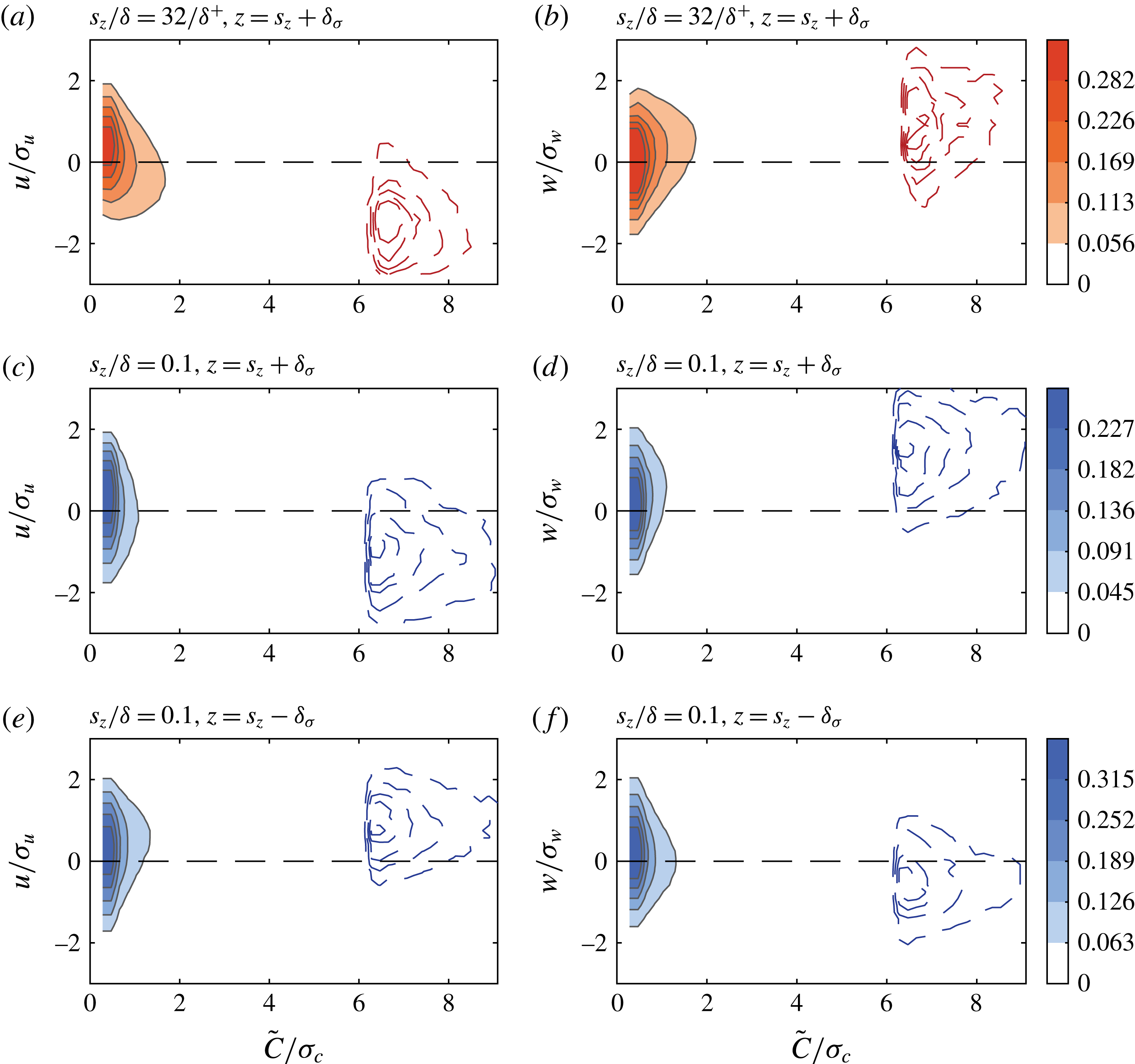
Joint probability density functions (j.p.d.f.s) of instantaneous concentration
 $\tilde{C}$
and either of three velocity fluctuations (
 $u,v,w$
) are computed. For the ground-level source,
 $s_{z}/\unicode[STIX]{x1D6FF}=32/\unicode[STIX]{x1D6FF}^{+}$
, figure 10(a,b) plots the contours of j.p.d.f.s of
 $u$
and
 $c$
, and
 $w$
and
 $c$
, respectively. These j.p.d.f.s are obtained at a location
 $z=s_{z}+\unicode[STIX]{x1D6FF}_{\unicode[STIX]{x1D70E}}$
, i.e. one plume half-width above the centreline. The j.p.d.f. of
 $v$
and
 $c$
is found to be symmetric about
 $v=0$
and hence is not shown here. In contrast to the conventional j.p.d.f., we have used instantaneous concentration (
 $\tilde{C}$
) rather than fluctuating concentration (
 $c$
) to always have a positive value for concentration. By adopting this approach, it is easier to quantify the contribution of positive and negative velocity fluctuations (
 $u$
,
 $v$
and
 $w$
) to high instantaneous concentration events. Further, the j.p.d.f.s between velocity and concentration fluctuation (
 $c$
) are qualitatively similar to the results presented in figure 10 and can be obtained simply by shifting the horizontal axis to the left by a value equal to the mean concentration.
In each plot of figure 10, filled contours show the j.p.d.f. obtained from the full signal, whereas the dashed contour lines show the corresponding j.p.d.f. calculated from portions of the signals when the instantaneous concentration is above a certain threshold (here, taken as
 $6\unicode[STIX]{x1D70E}_{c}$
). Further, it is important to note that the levels of filled contours and the dashed contours are represented by the same colour bar. In this conditional representation, dashed contours represent the combined probability of velocity and concentration fluctuations when concentration is high. It is observed that the j.p.d.f. of
 $u$
and
 $\tilde{C}$
computed from Cobra probe and PID measurements is in excellent agreement with those obtained from single hotwire and PID experiments. Further it is seen that, for the ground source and measurements above the plume centreline,
 $u$
fluctuations are negative when
 $\tilde{C}$
is high (figure 10
a), and this corresponds well with positive
 $w$
fluctuations and high
 $\tilde{C}$
(cf. figure 10
b). Thus, high-concentration events above the plume source height are associated with negative
 $u$
and positive
 $w$
, with an overall negative
 $\overline{uw}$
.
These observations are also true in the case of elevated sources, as evident from figure 10(c–f) for a source at
 $s_{z}/\unicode[STIX]{x1D6FF}=0.1$
. Here, the j.p.d.f.s are obtained from two locations that are at a distance of a plume half-width on either side of the plume centreline, i.e.
 $z=s_{z}\pm \unicode[STIX]{x1D6FF}_{\unicode[STIX]{x1D70E}}$
. Above the plume centreline, the sign preference for
 $u$
and
 $w$
fluctuations remain the same for the elevated source as it was for the ground-level source. However, below the plume centreline, high-concentration events are concurrent with positive
 $u$
fluctuations and negative
 $w$
fluctuations. The overall contribution of these events is still negative towards mean
 $\overline{uw}$
. These observations support our hypothesis of local transport by wall-normal motions, i.e.
 $w$
fluctuations and associated shear stress (
 $\overline{uw}$
) are responsible for vertical spread of the plume.
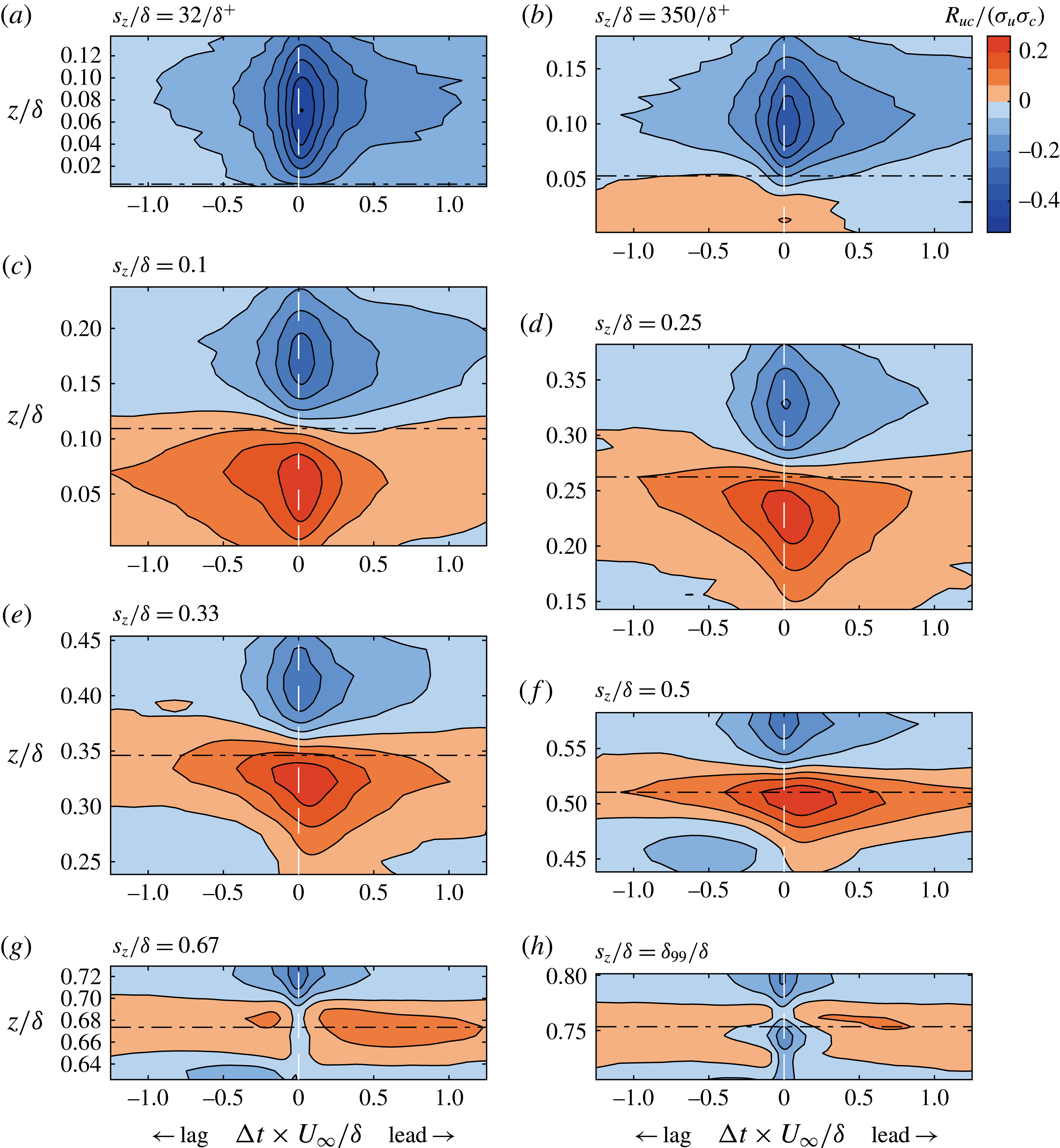
Contour maps of cross-correlation coefficient,
 $R_{uc}/(\unicode[STIX]{x1D70E}_{u}\unicode[STIX]{x1D70E}_{c})$
. The horizontal black dot-dashed line in each subplot indicates the source location.

4.3 Velocity–concentration cross-correlation
The cross-correlation function
 $R_{uc}$
between the fluctuating
 $u$
and
 $c$
is defined as
 $$\begin{eqnarray}R_{uc}(\boldsymbol{x},\unicode[STIX]{x0394}t)=\overline{u(\boldsymbol{x},\boldsymbol{t})\,c(\boldsymbol{x},t+\unicode[STIX]{x0394}t)}.\end{eqnarray}$$
Similar to
 $R_{ii}$
in § 3.2,
 $R_{uc}$
is different for different source heights and in our single-point measurements varies with
 $z$
. The results for
 $R_{uc}/(\unicode[STIX]{x1D70E}_{u}\unicode[STIX]{x1D70E}_{c})$
are presented as contour maps in figure 11 for the eight source heights. Note that time shift
 $\unicode[STIX]{x0394}t$
is normalised by
 $\unicode[STIX]{x1D6FF}/U_{\infty }$
and
 $\unicode[STIX]{x0394}t=0$
corresponds to distributions of
 $\overline{uc}$
in figure 9. Continuing from observations in figure 9, contours for positive correlation are below the centreline while contours for negative correlation are above the centreline. The contours also appear to be elongated along the horizontal as a footprint of large-scale velocity structures that are associated with high
 $\overline{uc}$
. It is clear that the correlation between
 $u$
and
 $c$
declines rapidly within a time scale that corresponds to a physical distance of approximately
 $(1{-}2)\unicode[STIX]{x1D6FF}$
if one considers free-stream velocity
 $U_{\infty }$
as the convection velocity. Thus, the elongated contours in figure 11 suggest that, although concentration events are relatively smaller than large-scale turbulent motions, they correlate well over extents of
 $O(1\unicode[STIX]{x1D6FF})$
. Therefore, large-scale coherent features are of significance for understanding the mechanisms of scalar transport.
Further, for source heights up to and including
 $s_{z}/\unicode[STIX]{x1D6FF}=0.5$
, there is a noticeable asymmetry in negative
 $R_{uc}$
above the plume centreline, i.e. the contours extend towards positive
 $\unicode[STIX]{x0394}t$
. In contrast (for
 $s_{z}/\unicode[STIX]{x1D6FF}=350/\unicode[STIX]{x1D6FF}^{+}$
, 0.1 and 0.25), the asymmetry for the positive contours is on the opposite side, i.e. the contours extend towards negative
 $\unicode[STIX]{x0394}t$
. In general, it is inferred that, above the source height, large-scale low-speed velocity structure has a lead over regions of significant concentration. Similarly, below the source height, large-scale high-speed velocity regions are lagging behind peak concentration events.
(a,d) Distribution of
 $\overline{uc}$
as a function of
 $\unicode[STIX]{x1D709}$
for two source heights,
 $s_{z}/\unicode[STIX]{x1D6FF}=350/\unicode[STIX]{x1D6FF}^{+}$
and
 $s_{z}/\unicode[STIX]{x1D6FF}=0.1$
, respectively. (b,c,e,f) In other plots:
 $f\unicode[STIX]{x1D6F7}_{uu}/\overline{u^{2}}$
, (green) dotted line;
 $f\unicode[STIX]{x1D6F7}_{cc}/\overline{c^{2}}$
, (blue) dashed line;
 $f\unicode[STIX]{x1D6F7}_{uc}/|\overline{uc}|$
, (red) dot-dashed line; and
 $\unicode[STIX]{x1D703}$
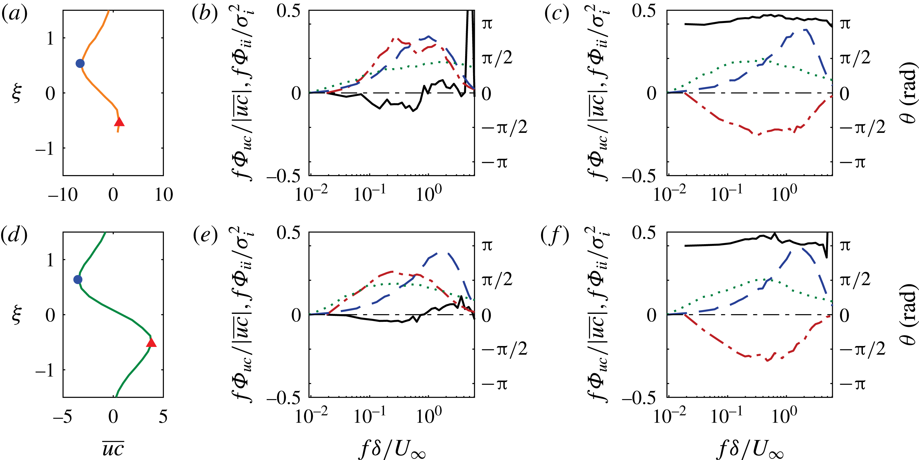
, (black) solid line. In (b,e)
 $\overline{uc}$
is maximum below
 $\unicode[STIX]{x1D709}=0$
; and in (c,f)
 $\overline{uc}$
is minimum above
 $\unicode[STIX]{x1D709}=0$
.

4.4 Pre-multiplied cross-spectral density
In this section, further evidence is sought for the relative lead/lag observed between velocity and concentration in figure 11 by examining cross-spectral density. The cross-correlation function
 $R_{uc}$
and the cross-spectra
 $\unicode[STIX]{x1D6E4}_{uc}$
are Fourier-transform pairs related as
 $$\begin{eqnarray}\frac{1}{2}\unicode[STIX]{x1D6E4}_{uc}(f)=\frac{1}{2\unicode[STIX]{x03C0}}\int _{-\infty }^{\infty }R_{uc}(t)\text{e}^{-\text{j}\,ft}\,\text{d}t.\end{eqnarray}$$
The quantity
 $\unicode[STIX]{x1D6E4}_{uc}(f)$
is in general complex, and it can be expressed as
 $\unicode[STIX]{x1D6E4}_{uc}(f)=\unicode[STIX]{x1D6F7}_{uc}(f)+\text{j}\unicode[STIX]{x1D6F9}_{uc}(f)$
, where
 $\unicode[STIX]{x1D6F7}_{uc}$
and
 $\unicode[STIX]{x1D6F9}_{uc}$
are the magnitudes of the real and imaginary components. Based on this definition of
 $\unicode[STIX]{x1D6E4}_{uc}$
, we can obtain the phase angle (
 $\unicode[STIX]{x1D703}$
) between
 $u$
and
 $c$
from the ratio of the imaginary and real parts as
 $$\begin{eqnarray}\unicode[STIX]{x1D703}(f)=\text{tan}^{-1}\left\{\frac{\unicode[STIX]{x1D6F9}_{uc}(f)}{\unicode[STIX]{x1D6F7}_{uc}(f)}\right\}.\end{eqnarray}$$
Given the definition of
 $R_{uc}$
in (4.1), a positive
 $\unicode[STIX]{x1D703}$
implies that
 $u$
leads
 $c$
, and a negative
 $\unicode[STIX]{x1D703}$
will indicate
 $u$
lags
 $c$
. Further, it is only the real component of
 $\unicode[STIX]{x1D6E4}_{uc}(f)$
, i.e.
 $\unicode[STIX]{x1D6F7}_{uc}$
, that contributes to scalar flux
 $\overline{uc}$
(a real quantity), and
 $\overline{uc}$
can be shown to be equal to the area under the pre-multiplied form of
 $\unicode[STIX]{x1D6F7}_{uc}$
as
 $\overline{uc}=\int _{0}^{\infty }f\unicode[STIX]{x1D6F7}_{uc}\text{d}\ln f$
. Henceforth, the discussion will be based on the real component of cross-spectra in the pre-multiplied form (
 $f\unicode[STIX]{x1D6F7}_{uc}$
).
For brevity, we will discuss the cross-spectra at two distinct points in profiles for
 $\overline{uc}$
when the source is located at
 $s_{z}/\unicode[STIX]{x1D6FF}=350/\unicode[STIX]{x1D6FF}^{+}$
and
 $s_{z}/\unicode[STIX]{x1D6FF}=0.1$
. These two distinct points correspond to the locations where
 $\overline{uc}$
is either maximum on minimum on either side of the plume centreline and indicated by solid symbols in figure 12(a,d). The other four panels (figure 12
b,c,e,f) plot
 $f\unicode[STIX]{x1D6F7}_{uu}/\overline{u^{2}}$
(dotted line),
 $f\unicode[STIX]{x1D6F7}_{cc}/\overline{c^{2}}$
(dashed line),
 $f\unicode[STIX]{x1D6F7}_{uc}/|\overline{uc}|$
(dot-dashed line) and the corresponding phase angle (
 $\unicode[STIX]{x1D703}$
, solid line) between
 $u$
and
 $c$
plotted together as functions of frequency. Figure 12(b) corresponds to positive maxima (solid triangle) and figure 12(c) corresponds to negative minima (solid circle) of
 $\overline{uc}$
in figure 12(a). Similarly figure 12(e) corresponds to positive maxima (solid triangle) and figure 12(f) corresponds to negative minima (solid circle) of
 $\overline{uc}$
in figure 12(d).
Figure 12(e) shows that the peak in
 $\unicode[STIX]{x1D6F7}_{uu}$
occurs at lower frequency than
 $\unicode[STIX]{x1D6F7}_{cc}$
as expected from the discussion in § 3.3. The cross-spectra, which receive contributions from both
 $u$
and
 $c$
, however, peak at a frequency that is closer to the peak frequency of
 $u$
. Consistent with the results of figure 9(b), where we observed that large-scale velocity fluctuations
 $u_{L}$
contribute significantly to
 $\overline{uc}$
,
 $\unicode[STIX]{x1D6F7}_{uc}$
indeed mimics
 $\unicode[STIX]{x1D6F7}_{u}$
more closely than
 $\unicode[STIX]{x1D6F7}_{c}$
, and obtains most of its contributions from lower frequencies of
 $u$
. This suggests that indeed the scalar is ‘passive’ for its contributions to the flux. This feature, however, is not observed for the measurement point close to the wall (figure 12
b), where dominant frequencies for
 $\unicode[STIX]{x1D6F7}_{uc}$
are closer to those for
 $\unicode[STIX]{x1D6F7}_{c}$
and there the concentration length scales dominates. This is due to the wall effect, where there is zero flux of concentration.
Further, in figure 12(c,f), corresponding to
 $\overline{uc}<0$
, it is evident that the magnitude of
 $f\unicode[STIX]{x1D6F7}_{uc}/|\overline{uc}|$
is negative across the entire range of frequency and, more importantly, the phase angle is close to
 $\unicode[STIX]{x03C0}$
. This implies that
 $u$
and
 $c$
are out of phase, which contributes to negative scalar flux in that region. Also, the phase
 $\unicode[STIX]{x1D703}$
is positive, which tells us that
 $u$
leads
 $c$
. Likewise, in the positive flux region below the plume centreline (figure 12
b,e), it is seen that
 $\unicode[STIX]{x1D703}$
is predominantly close to zero, suggesting that
 $u$
and
 $c$
are mostly in phase contributing to the positive value of
 $\overline{uc}$
. Also, for most of the frequencies that contributed to
 $\overline{uc}$
, the phase is negative (slightly below
 $0$
) showing that
 $u$
is lagging
 $c$
. These observations substantiate the proposition that, below the centreline of the plume, high-speed regions are lagging high-concentration regions and contribute to the positive concentration flux, while above the centreline low-momentum structures lead high-concentration regions and contribute to negative flux. The phase information obtained via cross-spectra analysis lends support to the lead/lag between
 $u$
and
 $c$
observed in the two-dimensional cross-correlation maps presented in figure 11. Furthermore, figures 11 and 12 represent the same information; however, the former is in physical space while the latter is in spectral space.
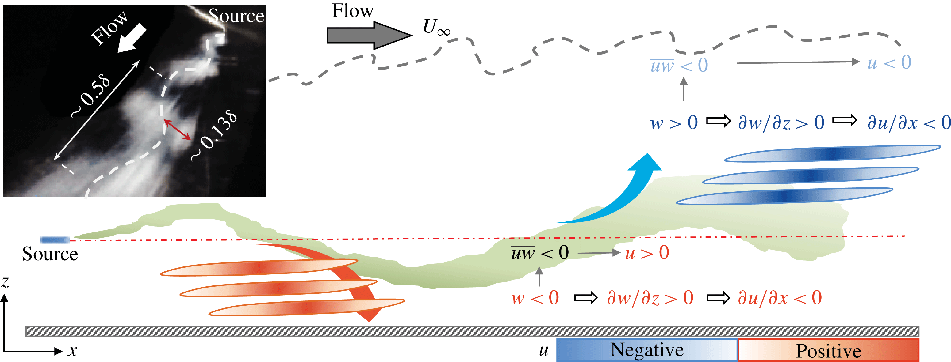
Relative arrangement of large-scale velocity structures around a decaying meandering plume shown in green. Low- and high-speed structures are depicted as blue and red regions in the schematic, respectively. Inset: A flow visualisation of the plume released at
 $s_{z}/\unicode[STIX]{x1D6FF}\approx 0.4$
, and captured by a ‘Go-Pro’ series wide-angle view camera. Note that the direction of flow is indicated by the white arrow and the meandering of the plume is shown by a dashed line.

5 Discussion and conclusions
5.1 A phenomenological model
In the previous sections statistical results for the integral time scales, scalar flux, cross-correlation and relative organisation of instantaneous velocity and concentration in the flow were discussed. It becomes necessary now to collate those results and develop a unified view of flow mechanisms that support our observations. This is achieved through a simplified physical model of the plume as presented in figure 13, which shows a plume emitted from a source that disperses about its local centre (i.e. become wider in size) and meanders or oscillates roughly about the centreline. Note that this model is only valid for sources located in the fully turbulent region (i.e. say below
 $z/\unicode[STIX]{x1D6FF}\approx 0.6$
) and not for a ground-level source. The wall reduces the meandering effect and, due to the zero flux condition at the wall, results in higher local concentration levels (e.g. Csanady Reference Csanady1973). We also would like to mention that flow visualisations (in the same set-up using visible smoke instead of the tracer gas) clearly shows that the plume meanders, although in the schematic the extent of meander is accentuated. The meandering plume model has been used in the past to provide quantitative information on statistics of a scalar (e.g. Gifford Reference Gifford1959), however, not for studying the velocity–scalar interaction, which is our aim here. Three main results are explained below using this model:
(i) In figure 9(a), it is found that scalar flux
 $\overline{uc}$
is negative above the plume centreline and positive below. As indicated in figure 13, the meandering, which is caused by the
$w$
fluctuations, carries the plume up (
$w>0$
) or down (
$w<0$
). The j.p.d.f.s in figure 10 attest to this behaviour for high concentration levels. Since the Reynolds shear stress
$\overline{uw}<0$
, when
$w$
is negative,
$u$
is likely to be positive and vice versa. Owing to the meandering, given the assertion that
$u$
is negative and positive when the plume is above and below, respectively, the flux
$\overline{uc}$
has to follow the sign of
$u$
fluctuation (since
$\tilde{C}$
is positively skewed), hence the resultant distribution in figure 9(a).
(ii) A ‘double peak’ in the wall-normal distribution of
$\unicode[STIX]{x1D70F}_{c}$
was observed in figure 6. Also, there is a lack of a secondary peak below the plume centreline. Given similar mixing characteristics, if the plume spends more time at a location, the tendency is to have a larger
$\unicode[STIX]{x1D70F}_{c}$
. Therefore, it is not surprising that one peak in
$\unicode[STIX]{x1D70F}_{c}$
appears close to the centreline, because, although the plume is meandering, it is still primarily at the centreline. However, the meandering implies that the plume will also spend more time at the edges (although an exaggeration, in a manner similar to a pendulum). Assuming that the local convection velocity of the scalar is the same as the local flow velocity (since it is a passive scalar), the plume above the centreline is convected with motions that have
$u<0$
and thus spends more time at the probe, hence giving rise to the second peak in
$\unicode[STIX]{x1D70F}_{c}$
. Furthermore, when the plume is below the centreline, the corresponding
$u$
fluctuations that convects it are positive, and therefore a relatively smaller time is spent at the probe, compared to when the plume is above the centreline – hence the asymmetry in the
$\unicode[STIX]{x1D70F}_{c}$
distribution about the centreline.(iii) In figure 11, say for
$s_{z}/\unicode[STIX]{x1D6FF}=0.1$
corresponding to figure 11(c), we observed a lead for negative (blue) contours of
$R_{uc}$
above the centreline but a lag for positive (red) contours below the centreline. This suggests that the low-speed structures lead the plume in the region above the centreline while high-speed structures are lagging behind the plume below its centreline. Let us consider
$w>0$
(ejection-like events) indicated in figure 13, which cause the plume to meander above the centreline. With such events, the gradient
$\unicode[STIX]{x2202}w/\unicode[STIX]{x2202}z>0$
(for the plume to spread upwards) and from (two-dimensional) continuity equation, it can be inferred that
$\unicode[STIX]{x2202}u/\unicode[STIX]{x2202}x<0$
. The two conditions
$u<0$
and
$\unicode[STIX]{x2202}u/\unicode[STIX]{x2202}x<0$
imply that the tail of a large-scale low-speed structure is well correlated with concentration fluctuations above the centreline of the plume, i.e. peak negative
$u$
fluctuation events lead peak concentration events. Likewise, sweep-like events with
$w<0$
and
$\unicode[STIX]{x2202}w/\unicode[STIX]{x2202}z>0$
convect the plume downwards. The associated two conditions for streamwise velocity fluctuations,
$u>0$
and
$\unicode[STIX]{x2202}u/\unicode[STIX]{x2202}x<0$
imply that the frontal portions of a high-speed structure are well correlated with concentration fluctuations below the centreline of a meandering plume.


In order to provide physical evidence for the role of transverse and vertical velocity fluctuations in plume meandering, we have conducted smoke visualisation of the plume released at
 $z/\unicode[STIX]{x1D6FF}=0.2$
. One of the time instants is shown in the inset of figure 13, which clearly shows the meandering behaviour of the plume. It is found that the wavelength of the meander is approximately
 $0.5\unicode[STIX]{x1D6FF}$
at this instant. From recent measurements in high-Reynolds-number turbulent boundary layers (Baidya et al.
Reference Baidya, Philip, Hutchins, Monty and Marusic2017), the dominant streamwise length scale of
 $w$
fluctuations is found to scale as
 $\unicode[STIX]{x1D706}_{x_{w}}\approx 2z$
, which for
 $z=0.2\unicode[STIX]{x1D6FF}$
gives
 $\unicode[STIX]{x1D706}_{x_{w}}\approx 0.4\unicode[STIX]{x1D6FF}$
. This indicates that the meandering length scale is of the same order as that of the vertical velocity length scale, which is suggestive that the vertical velocity plays a key role in plume meandering, in support of our physical model.
An obvious question that follows is how does the time scale of plume meandering compare against the integral time scale of concentration,
 $\unicode[STIX]{x1D70F}_{c}$
, previously discussed in § 3.2. In order to estimate the time scale of plume meandering, we need an appropriate velocity scale for its travel in the transverse or lateral direction, which is possible only by Lagrangian tracking of the scalar, and we have not performed such a measurement. However, to compare with the Eulerian estimate
 $\unicode[STIX]{x1D70F}_{c}$
, the meandering time of the plume can be indirectly estimated by two approaches. First, we are interested in the time over which the meandering plume goes past a stationary probe, denoted here as
 $\unicode[STIX]{x1D70F}_{m_{E}}$
. Here we consider the local convection velocity
 $U(z)$
to be the appropriate velocity scale. For
 $z/\unicode[STIX]{x1D6FF}=0.2$
,
 $U(z)\approx 8.56~\text{m}~\text{s}^{-1}$
and with the meandering streamwise length scale set to be
 $0.5\unicode[STIX]{x1D6FF}$
, we get
 $\unicode[STIX]{x1D70F}_{m_{E}}U_{\infty }/\unicode[STIX]{x1D6FF}\approx 0.6$
. This is approximately three times the integral concentration time scale
 $\unicode[STIX]{x1D70F}_{c}$
(cf.
 $\unicode[STIX]{x1D70F}_{c}U_{\infty }/\unicode[STIX]{x1D6FF}\approx 0.2$
in figure 5
b). A second approach, and perhaps a more relevant meandering time scale closer to the Lagrangian viewpoint, is the time scale at which the plume meanders up and down. For the corresponding velocity scale, it is justified to consider the r.m.s. of
 $w$
fluctuations (
 $\unicode[STIX]{x1D70E}_{w}$
) as a first approximation since the scalar is passive. Further, the appropriate length scale is the amplitude of the meandering in the
 $z$
direction, here considered as
 $2\unicode[STIX]{x1D6FF}_{\unicode[STIX]{x1D70E}}=0.13\unicode[STIX]{x1D6FF}$
(cf. figure 3, which is further confirmed via smoke visualisation in figure 13). As such, the time scale of plume meandering in the Lagrangian reference frame can be approximated as
 $\unicode[STIX]{x1D70F}_{m_{L}}=0.13\unicode[STIX]{x1D6FF}/\unicode[STIX]{x1D70E}_{w}$
(thus
 $\unicode[STIX]{x1D70E}_{w}U_{\unicode[STIX]{x1D70F}}/\unicode[STIX]{x1D708}\approx 1.4$
at
 $z/\unicode[STIX]{x1D6FF}=0.2$
(Baidya et al.
Reference Baidya, Philip, Hutchins, Monty and Marusic2017)), which in non-dimensional form becomes
 $\unicode[STIX]{x1D70F}_{m_{L}}U_{\infty }/\unicode[STIX]{x1D6FF}\approx 2.5$
. This estimate is an order of magnitude larger than
 $\unicode[STIX]{x1D70F}_{c}U_{\infty }/\unicode[STIX]{x1D6FF}$
. Therefore, it is reasonable to interpret that meandering occurs on a much longer time scale in comparison to the integral time scale
 $\unicode[STIX]{x1D70F}_{c}$
. Admittedly the proposed velocity–concentration model is simplified and perhaps preliminary, and further work is required to make it quantitative. Nevertheless, it provides a consolidated summary of observations made in a consistent manner.
6 Conclusions
High-quality measurements (with good spatial and temporal resolution) of velocity and concentration fluctuations downstream of a plume released at different heights in a turbulent boundary layer are reported here with a specific aim of understanding the role of velocity structures in the local transport of a scalar. A comparison of mean and r.m.s. profiles for different source heights in the boundary layer suggest that all elevated plumes can be fitted to the reflected Gaussian distribution while ground-level plumes exhibit an exponential distribution. This is found to be consistent with the previous studies of Fackrell & Robins (Reference Fackrell and Robins1982) and Nironi et al. (Reference Nironi, Salizzoni, Marro, Mejean, Grosjean and Soulhac2015). Temporally resolved concentration data enabled us to compute integral time scales of concentration across the plume, and it is observed that the integral time scales of concentration fluctuations are nominally
 $O(10)$
smaller than those of velocity fluctuations, implying that concentration structures have shorter length scales. Further, the streamwise concentration flux is found to be negative and positive above and below the plume centreline, respectively. Cross-correlation results and the phase relationship between velocity and concentration fluctuation indicate that there is a predominant phase angle of
 $\unicode[STIX]{x03C0}$
between
 $u$
and
 $c$
above the plume centreline where
 $u$
leads
 $c$
, while this trend gets reversed below the centreline. All these observations are explained using a physical model that is based on arrangement of instantaneous velocity and scalar structures.