





Introduction
Applications enabled by emerging wireless technologies such as 5G and WiFi have led to enormous growth in recent years, with exciting use cases emerging in integrated sensing and communication and autonomous driving [Reference Liu, Cui, Masouros, Xu, Han, Eldar and Buzzi1]. These technologies require high-fidelity testing and optimization, both in pre- and post-deployment, in order to meet stringent performance targets. A typical post-deployment test method in 5G and legacy communication systems is drive testing, whereby performance logs are generated and analyzed to identify potential bottlenecks. An alternative pre-deployment approach which can reduce the number of physical drive tests required is virtual drive testing (VDT) [Reference Schiller, Knoll, Mocker and Eibert2, Reference Fan, Carton, Kyösti and Pedersen3]. Site-specific models of the radio channel are a natural tool for VDT, with ray tracing (RT) simulations being particularly attractive due to their ability to achieve good accuracy in terms of key performance indicators including pathloss, angular and delay spread [Reference Mbugua, Chen, Raschkowski, Thiele, Jaeckel and Fan4]. RT simulations have much lower computational complexity as compared to full-wave models but, given the growing complexity of environment representations, still require significant run-times. Trade-offs between accuracy and computation times are still typically required.
In the particular case of VDT, an important observation is that neighboring frames often display coherence, that is, the set of rays arriving at the receiver (Rx) is similar. This is especially the case when the inter-frame distance is of the order of a small number of wavelengths. This has formed the basis of a number of approaches to reducing the computational burden associated with RT in the context of moving objects, specifically by either reducing the cost of constructing and validating rays, or by interpolating their associated field amplitudes. In particular, this is exploited in [Reference Wang and Manocha5] in the context of dynamic RT in order to minimize the need to rebuild the bounding volume hierarchy and also to perform ray intersection checks, the latter being achieved by a process of propagation path caching. In [Reference Hussain and Brennan6, Reference Hussain and Brennan7], a visibility table, defined as comprising edges and faces which are visible to the Tx and Rx, is pre-computed and used to accelerate RT simulation in urban microcellular scenarios, while in [Reference Bilibashi, Vitucci and Degli-Esposti8–Reference Quatresooz, Demey and Oestges10] rays identified in a single RT simulation are extrapolated based on the motion of both the interaction points and dynamic objects, allowing a dynamic RT model to be created. A major challenge in this approach is the specification of the coherence time, that is, the length of time for which the rays identified in the initial RT remain valid. Hussain and Brennan [Reference Hussain and Brennan11] outline an approach in which a well-defined geographical zone called a lit region is identified for each reflected and diffracted ray. By the laws of geometric optics and Uniform Theory of Diffraction (UTD), a valid ray can only potentially exist for receiver points lying inside this region. Combined with the complementary notion of shadow regions, this facilitates the rapid identification of points along a mobile receiver’s trajectory to which reflected and diffracted rays can feasibly propagate, thereby eliminating the need for ray validation at points that are in shadow or outside the lit region. Hussain and Brennan [Reference Hussain and Brennan6] extended this to the case of a moving transmitter, an extension which requires the efficient specification of the varying geographical extent of the lit region.
Complementary to these approaches, which attempt to reduce the burden associated with the geometrical identification of rays, is the idea of numerically interpolating their (complex-valued) field amplitudes. Linear interpolation is used in [Reference Nuckelt, Schack and Kürner12] to interpolate the complex amplitude of the line of sight and other multipath components. A potential shortcoming of this strategy is when it is applied to diffracted rays whose complex amplitude can vary rapidly in the vicinity of shadow boundaries. In addition, it employs simple heuristic approaches to situations where rays either appear or disappear due to shadowing along the route. A similar approach is outlined in [Reference Zentner and Mucalo13] in which ray entities (i.e. collections of rays grouped by the interaction mechanism) are proposed. Interpolation of rays is identified as a potential benefit of this approach, but it is not explicitly performed.
In this paper, aspects of both approaches are combined. Firstly, lit regions in which specific rays exist are identified [Reference Hussain and Brennan11], thereby removing many cumbersome visibility and validation checks. Secondly, highly accurate (non-linear) mathematical interpolation is used to create simple models for the field amplitudes within these regions, removing the requirement to explicitly trace and process a ray to each receiver location within the region. This paper is an expanded version of [Reference Brennan, Mbugua, Chen and Hussain14] wherein the cubic spline interpolation models developed improve upon the simple polynomial models presented in the previous work, as they are more stable as the number of interpolation points is increased.
This paper presents an interpolation-based approach in which reflected and diffracted rays are approximated individually within their so-called lit region (defined as the region in space in which the ray can feasibly exist given the laws of geometric optics and UTD). The paper is organized as follows. Fields associated with rays vary rapidly as the Rx moves, but in Section “Ray interpolation” it is outlined how the fast-moving phase can be extracted, leaving residual fields which can be factored into several terms, each of which can be approximated accurately using interpolation. Section “Interpolation methods” introduces two interpolation approaches, polynomial interpolation and cubic spline interpolation. Section “Validation and comparison of interpolation methods” validates the method in the context of reflection and diffraction from a single building face. More complex examples involving a street canyon are presented in Section “Results.” We close with conclusions and by identifying future work.
Ray interpolation
An accurate and rapid approximation to the fields associated with a ray can be made using interpolation. The key observation in each case is that the associated field components comprise the product of a relatively slowly varying amplitude term with a rapidly varying complex exponential term. However, the phase of the latter term varies relatively slowly. The amplitude and phase terms can thus be interpolated, a process which is detailed for reflected and diffracted rays respectively in the next subsections.
Interpolation of reflected rays
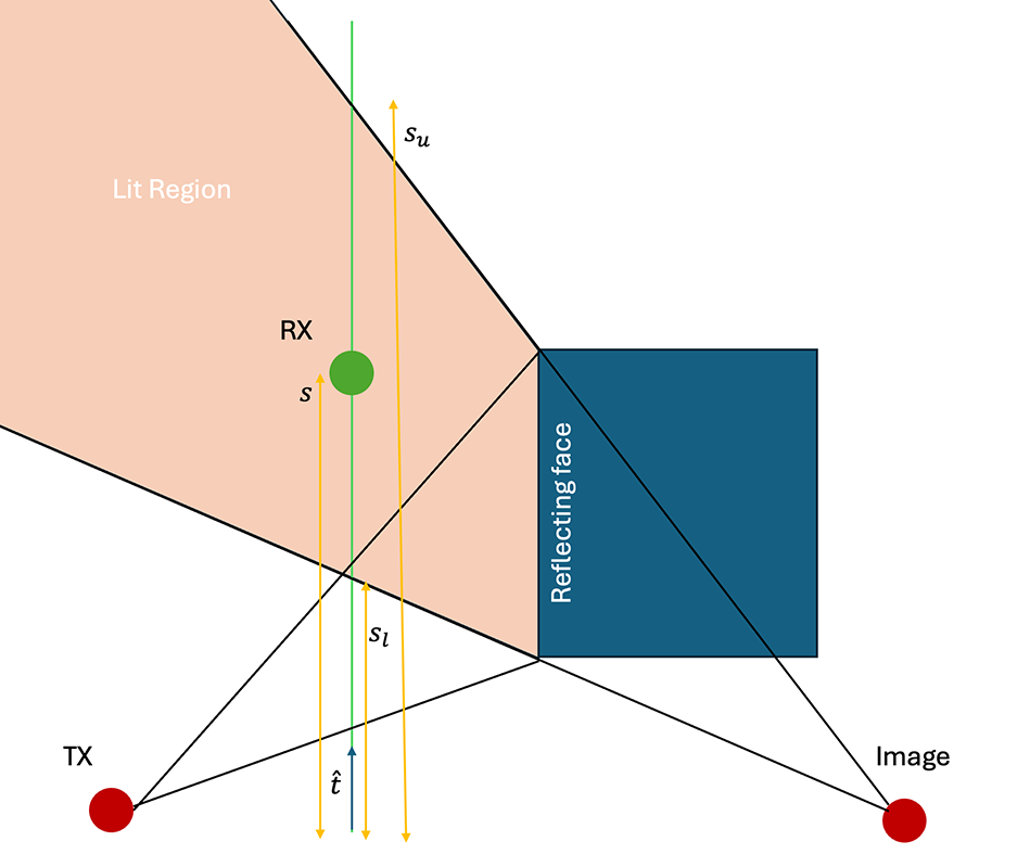
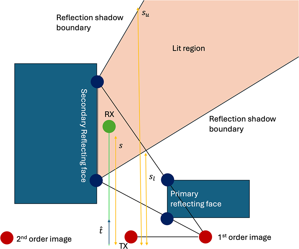
Consider the situation depicted in Figure 1. A receiver is traveling on a linear trajectory (green line) in the direction  $\hat t$. Its distance along this trajectory is given by
 $s$. It enters the lit region associated with a reflecting face at
 $s=s_l$, at which point it receives a reflected ray. It will continue to receive this reflected ray until it exits the lit region at
 $s=s_u$. The laws of geometric optics determine both
 $s_l$ and
 $s_u$, while the precise definition of the lit region depends on the order of the reflection. Figure 2 illustrates its construction for second (and higher) order reflections. The electric field associated with a reflected ray is given by
 \begin{equation}
{\mathbf E}^{r} \left( s \right) = \left[ \begin{array}{cc}
\Gamma_\perp & 0 \\ 0 & \Gamma_\parallel
\end{array} \right] \left[ \begin{array}{c}
E_\perp^i \\ E_\parallel^i \end{array}
\right] \frac{R_1}{R_1 + R_2 } e^{-\jmath k R_2},
\end{equation}
where  $\Gamma_\parallel, \Gamma_\perp$ are the parallel and perpendicular reflection coefficients and
 $E_\perp^i , E_\parallel^i $ are the perpendicular and parallel components of the incident electric field at the reflection point.
 $R_1, R_2$ are, respectively, the distances from the source to the reflection point and from the reflection point to the field point (which is located a distance
 $s$ along the trajectory). The complex exponential term
 $e^{-\jmath k R_1}$ can be factored from the incident field leaving
 \begin{equation}
{\mathbf E}^{r} \left( s \right) = {\mathbf A}(s) e^{-\jmath {\hat R}(s) }
\end{equation}
 \begin{equation}
= \left[ \begin{array}{c} A_\perp (s) \\ A_\parallel (s) \end{array} \right] e^{-\jmath k {\hat R}(s) },
\end{equation}
where
 \begin{equation}
A_\perp (s) = \Gamma_\perp \left| E_\perp^i \right| e^{\jmath \phi_\perp } \frac{R_1}{R_1 + R_2}
\end{equation}
 \begin{equation}
A_\parallel (s) = \Gamma_\parallel \left| E_\parallel^i \right| e^{\jmath \phi_\parallel } \frac{R_1}{R_1 + R_2}
\end{equation}
 \begin{equation}
\!\!\!\!\!\!\!\!\!\!\!\!\!{\hat R}(s) = k \left( R_1 + R_2 \right).
\end{equation}
 $\phi_\perp$ and
 $\phi_\parallel$ are slowly varying residual phase terms which remain after the rapidly varying phase terms
 $k \left(R_1 + R_2\right)$ are grouped together as
 $\hat R(s)$. The term
 $\hat R(s)$ (which is the total electrical length traveled by the reflected ray) varies slowly along the trajectory (although the complex exponential in Equation (2) for which it is the argument varies rapidly). Slow variations in spreading loss, reflection coefficient, antenna pattern, etc. are captured in
 $A_\perp (s)$ and
 $A_\parallel(s)$. All three slowly varying terms (
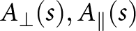 $A_\perp (s), A_\parallel(s)$, and
 $\hat R(s)$ ) can be approximated using either low-order polynomials or cubic splines as outlined in Section “Interpolation methods.”
A receiver trajectory (green line) passing through the lit region. The reflected ray (from the reflecting face) will only exist between the shadow boundaries  $s=s_l$ and
 $s=s_u$. Diffracted rays emanating from the edge of the reflecting face will exist along the entire route, but will exhibit discontinuities at the shadow boundaries.

Construction of the lit region for a higher-order reflection.

Interpolation of diffracted rays
The presence of the optical shadow boundaries, across which the diffracted fields are discontinuous (thereby compensating for the discontinuities in the geometric optics field), complicates the interpolation process for the fields associated with diffracted rays. In particular, smooth polynomials or cubic splines will not be able to model such a discontinuity. Instead, separate interpolation models are used for portions of receiver trajectory lying between each shadow boundary. Consider the case of diffraction from the south-west corner of the building in Figure 1. One interpolation model is created for field points between  $s =0$ and the reflection shadow boundary at
 $s = s_l$, and another model is created for points from
 $s = s_l$ onwards. A similar process is applied to diffraction from the north-west corner.
A field point located a distance  $s$ along the trajectory will receive a diffracted ray from one of the edges with electric field [Reference Balanis15]
 \begin{equation}
{\mathbf E}^d (s) =
\left[ \begin{array}{c}
E_{\beta_0}^d (s) \\
E_{\phi}^d (s)
\end{array}
\right]
\end{equation}
 \begin{equation}
\ \ \ \ \ \ \ \ \ =
{\mathbf B} (s) e^{-\jmath k R_2},
\end{equation}
where the term  $e^{-\jmath k R_2}$ accounts for the phase acquired in free-space propagation to the field point from the diffraction point and
 \begin{equation}
{\mathbf B} (s) =
\left[ \begin{array}{cc}
D_s & 0 \\
0 & D_h
\end{array}
\right]
\left[ \begin{array}{c}
E_{\beta^\prime_0}^{inc} \\
E_{\phi^\prime}^{inc}
\end{array}
\right]
G \left( R_1, R_2 \right)
\end{equation}
 \begin{equation}
\!\!\!\!\!\!\!\!\!\!\!\!\!\!\!\!\!\!\!\!\!\!\!\!\!\!\!\!\!\!\!\!\!\!\!\!\!\!=
\left[ \begin{array}{c}
B_{\beta_0}(s) \\
B_{\phi}(s) \\
\end{array}
\right].
\end{equation}
 $D_h$ and
 $D_s$ are the hard and soft diffraction coefficients, while
 $E_{\beta^\prime_0}^{inc}$ and
 $E_{\phi^\prime}^{inc}$ are the components of the incident field at the diffraction point, using an edge-based coordinate system, and the spreading term is given by
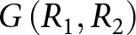 $G \left(R_1, R_2\right)$.
 $\beta_0$ and
 $\phi$ are angles which define the local coordinate system. More details of the derivation of these terms are available in [Reference Balanis15].
Factoring  $B$ into amplitude and complex exponential terms yields
 \begin{equation}
B_{\beta_0}(s) =
\left| B_{\beta_0} (s) \right| e^{\jmath \theta_1 (s) }
\end{equation}
 \begin{equation}
B_{\phi}(s) =
\left| B_{\phi} (s) \right| e^{\jmath \theta_2 (s) },
\end{equation}
where  $\left| B_{\beta_0} (s) \right|, \left| B_{\phi} (s) \right|, \theta_1(s), \theta_2 (s)$, and
 $R_2(s)$ are slowly varying quantities with respect to receiver motion and can thus be interpolated as per the techniques described in the next section.
Interpolation methods
The previous section outlined how the fields can be simply written in terms of a number of quantities that vary slowly with receiver motion and are thus amenable to approximation by interpolation. Two interpolation schemes are considered and compared in this paper: polynomial interpolation and cubic spline interpolation.
Polynomial interpolation
Assuming that the function to be approximated is  $f$, interpolation proceeds by sampling the function at discrete inputs
 $s_i$, producing corresponding outputs
 $f_i$. Given
 ${M+1}$ data points of the form
 $\left(s_i, f_i \right)$ for
 $i = 0 \dots M$, polynomial interpolation fits a polynomial of order
 $M$
 \begin{equation}
p(s) = a_0 + a_1 s + a_2 s^2 + \dots + a_M s^M \end{equation}
where the coefficients satisfy
 \begin{equation}
\left[
\begin{array}{cccc}
1 & s_0 & s_0^2 \dots s_0^M \\
1 & s_1 & s_1^2 \dots s_1^M \\
\vdots & \vdots & \vdots & \vdots \\
1 & s_M & s_M^2 \dots s_M^M \\
\end{array}
\right]
\left[
\begin{array}{c}
a_0 \\
a_1 \\
\vdots \\
a_M
\end{array}
\right]
=
\left[
\begin{array}{c}
f_0 \\
f_1 \\
\vdots \\
f_M
\end{array}
\right].
\end{equation}
Specification of the coefficients  $a_m$ for
 $ m = 0 \dots M$ thus requires field data at
 $M+1$ points in the lit region, obtained using exact RT to these points. Once the coefficients have been specified, they can be used to rapidly compute the reflected or diffracted fields at any point within the lit region as per Equations (2) and (8).
Cubic spline interpolation
A known problem with polynomial interpolation is its lack of stability when the number of data points grows, caused by the rapid variations associated with the higher-order terms (e.g.  $s^M$) as
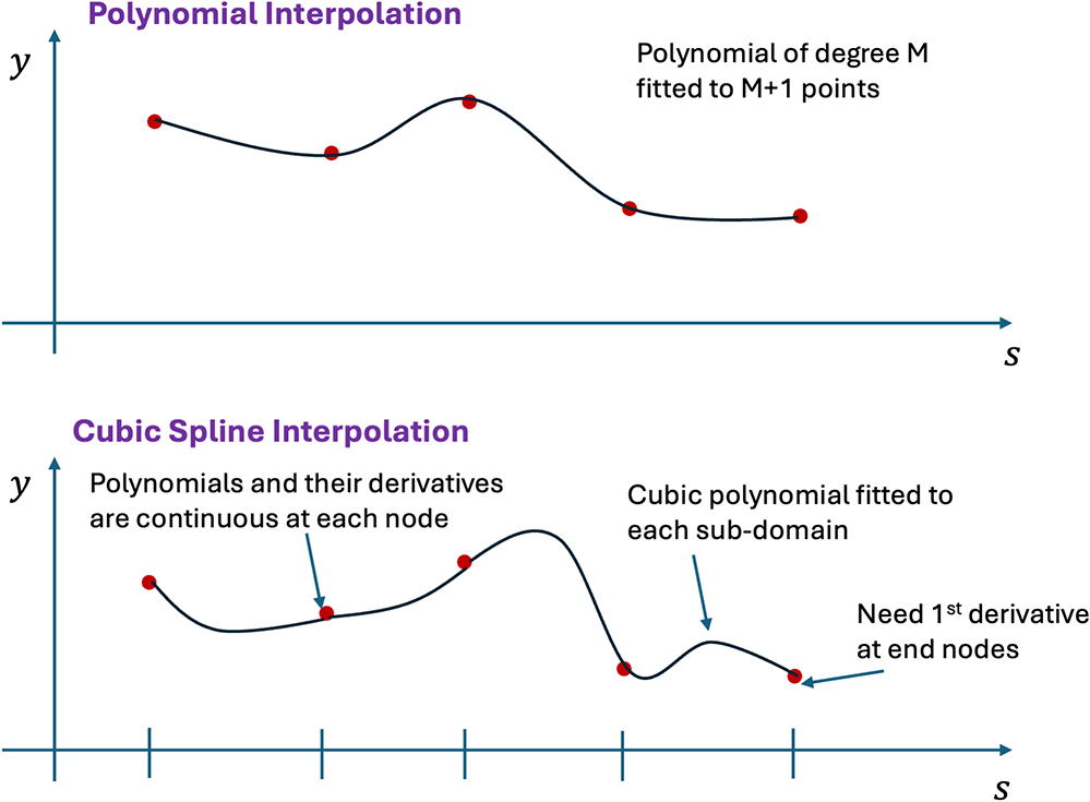
 $M$ grows. While the polynomial is guaranteed to pass through the particular data points used to compute the coefficients, large oscillations can nonetheless develop at intermediate points. A commonly used alternative, with a similar computational cost, is cubic spline interpolation. Referring to Figure 3, we see that
 $M+1$ data points can be used to either fit a single polynomial of degree
 $M$ through all points or a sequence of cubic polynomials over each of
 $M$ subdomains where the
 $i^{th}$ subdomain spans
 $s \in \left[ s_i, s_{i+1} \right]$. The cubic polynomial (referred to as “splines”) in sub-domain
 $i$ is given by
 \begin{equation}
p_i(s) = a_0 + a_1 s + a_2 s^2 + a_3 s^3
\end{equation}
where the four coefficients  $a_0,a_1,a_2$, and
 $a_3$ must be computed for each sub-domain. This is achieved by fitting
 $p_i(s)$ to the data points
 $(s_i,f_i)$ and
 $(s_{i+1},f_{i+1})$. In addition, splines in adjacent sub-domains are constrained to have continuous first and second derivatives at their common vertices. These constraints yield
 $2M + 2\left( M- 1 \right) = 4M-2$ equations. Given that a total of
 $4M$ coefficients are required, it is necessary to impose two further constraints. These take the form of specifying the function derivative at the end points, that is, requiring
 $p^\prime_0(s_0) = \eta_1$ and
 $p^\prime_{M-1} (s_M) = \eta_2$ for some boundary values
 $\eta_1$ and
 $\eta_2$. Cubic splines can be fit to a lit region by sampling
 $M$ points within the lit region, performing ray traces to obtain field information at each of the
 $M$ points and supplementing this with two extra ray traces at points very close to the start and end points of the lit region in order to numerically estimate the required derivative information at the boundaries.
Polynomial and cubic spline interpolation defined on  $M+1$ data points.

Validation and comparison of interpolation methods
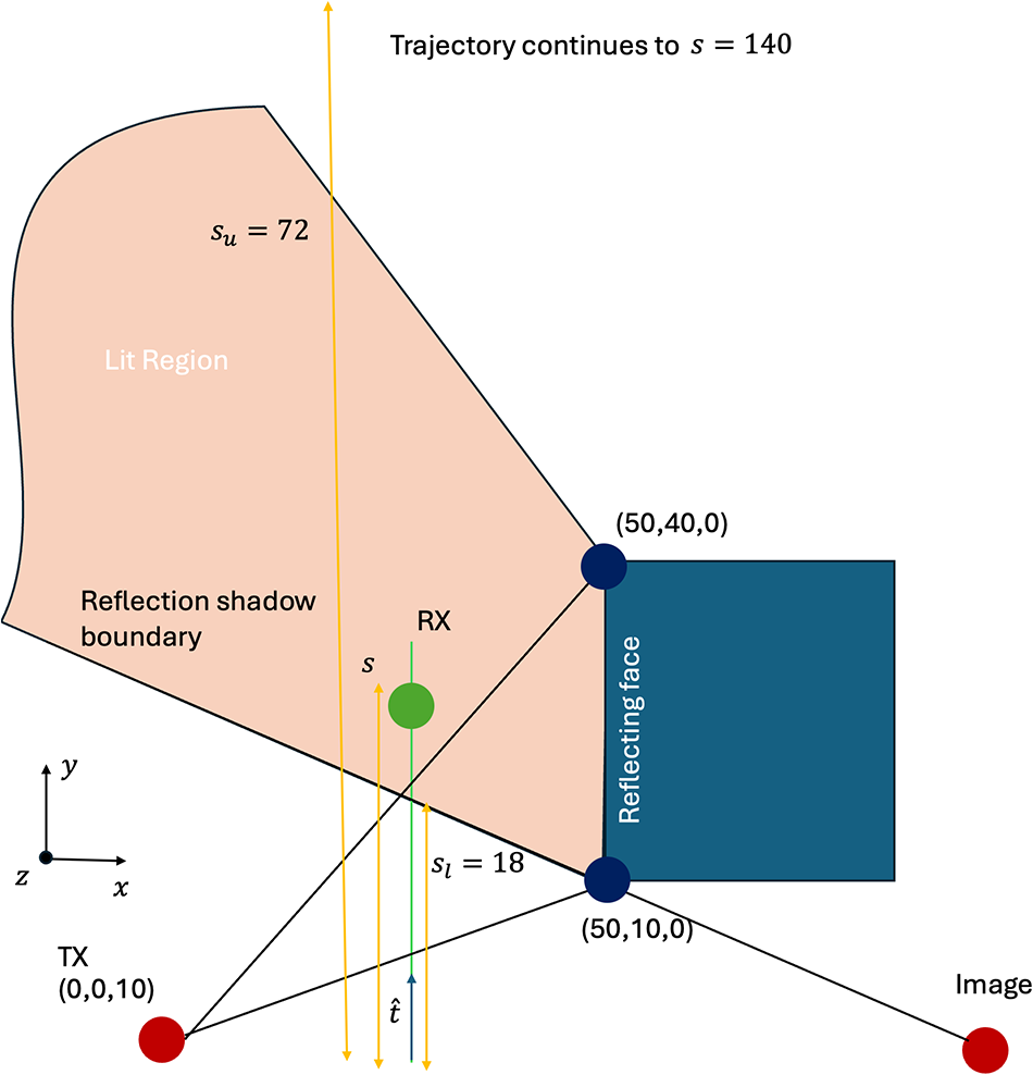
The model is validated by considering the example depicted in Figure 4.
Geometry for validation example. Receiver travels from  $s=0$ to
 $s=140$, passing through shadow boundaries at
 $s=18$ and
 $s=72$ as it does so.

Figure 4 Long description
A geometric setup for validation, featuring a trajectory and reflection shadow boundaries. The trajectory starts at a point labeled TX at coordinates zero, zero, ten, marked by a red dot. It travels through a reflection shadow boundary, indicated by a line and continues to a point labeled RX, marked by a green dot. The trajectory extends to s equals one hundred forty. A lit region is shown on the left, with a boundary labeled s subscript u equals seventy-two. A reflective face is depicted as a blue rectangle at coordinates fifty, forty, zero. The x-axis and y-axis are labeled, with the x-axis extending horizontally and the y-axis vertically. The diagram includes additional points and lines, such as x subscript l equals eighteen and a point at fifty, ten, zero, marked by a red dot. The setup demonstrates the interaction of the trajectory with the reflective surface and shadow boundaries.
A vertical dipole is located at  $(0, 0, 10)$ and radiates at 300 MHz. A rectangular building of height 40 m, and
 $\epsilon_r = 4$ is located with the south-west corner at
 $(50, 10, 0)$. A receiver moves along a trajectory
 $(x=10,y \in \left( 0, 140 \right),z=10)$ as shown, and single reflections and diffractions are considered from the leftmost face of the building. The receiver crosses reflection shadow boundaries at
 $s=18$ and
 $s=72$, and a reflected ray therefore exists for
 $s \in \left[ 18, 72 \right]$. As a reference, exact RT is used to compute the fields along a fine grid of 1200 points along the trajectory. To create the interpolated model of the reflected rays, an exact ray trace was performed at
 $M$ points through the lit region, and polynomial and spline approximations were created for the slowly varying quantities as outlined in Section “Interpolation of reflected rays.” A similar process was followed to create polynomial and spline interpolated models for the diffracted field. Equations (2) and (8) along with the interpolation models were used to approximate the electric fields along the same fine grid of points for which reference results were computed. The number of interpolation points,
 $M$, was varied in order to gauge how the interpolation accuracy is affected by the order of interpolation. For the case of reflected fields, interpolation was used in the lit region from
 $s=18$ to
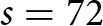 $s=72$. As outlined in Section “Interpolation methods,” data at
 $M$ interpolation points can be used to make a single polynomial of degree
 $M-1$ throughout the region or a cubic spline interpolation across each of
 $M-1$ subregions. In both cases, an exact ray trace is required for each of the
 $M$ interpolation points. In the case of cubic spline interpolation, a further two ray traces are required, one at the start and end of the interpolation region, in order to numerically estimate the derivative of the slowly varying field quantities at these end points. In order to gauge the accuracy of both the magnitude and phase of the fields, we examine the behavior of the real components of the field throughout the region. At each of the
 $N=1200$ points in the lit region, we compute the error as
 \begin{equation}
\epsilon (\vec r) = \left| \Re \{E_z (\vec r) \} - \Re \{\tilde E_z (\vec r) \} \right|
\end{equation}
where  $E_z$ is the exact
 $z$ component of the electric field while
 $\tilde E_z$ is the interpolated approximation to this quantity.
 $\bar \epsilon_p$,
 $\bar \epsilon_s$ are defined as the average error using polynomial interpolation and cubic spline interpolation, respectively, while
 $\epsilon_{p,max}$ and
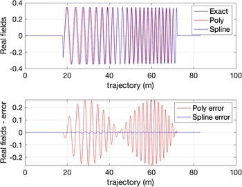
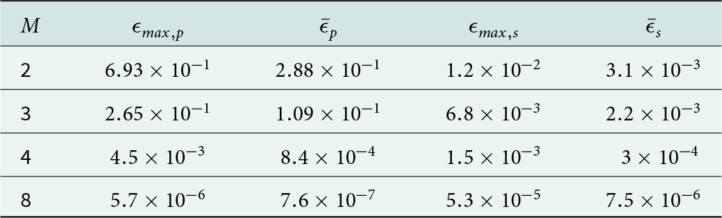
 $\epsilon_{s,max}$ are the maximum errors. Referring to Table 1, it is noted that the accuracy of both interpolation schemes increases as the number of interpolation points rises, as expected. Figure 5 shows the real part of the fields associated with the reflected ray in the lit region (
 $s \in \left(18,72) \right)$ for the case of
 $M=3$ (i.e. quadratic polynomial interpolation, and cubic splines defined over two intervals). Despite the low order of the interpolations, the agreement is almost perfect in the case of cubic splines (which essentially overlay the exact results in the top plot. This is more evident in the bottom plot, which shows the difference between the exact computation and the polynomial [red] and spline [blue] approximations). This simulation corresponds to the second row of Table 1.
Top: Exact and approximated reflected fields along a portion of the trajectory for the validation example. Black curve is the real value of the exact  $z$ component of the electric field. Red and blue are polynomial and cubic spline interpolated approximations (the latter effectively overlaying the exact values). Bottom: Error between exact and interpolated fields. Red is the error associated with the polynomial, while blue is the error given by the cubic spline approximation.

Reflection: Interpolation accuracy versus number of interpolation points

Table 1 Long description
Five columns list M and four error measures labeled epsilon max p, bar epsilon p, epsilon max s, and bar epsilon s. For M 2, epsilon max p is 6.93 times 10 to the minus 1, bar epsilon p is 2.88 times 10 to the minus 1, epsilon max s is 1.2 times 10 to the minus 2, and bar epsilon s is 3.1 times 10 to the minus 3. For M 3, the values are 2.65 times 10 to the minus 1, 1.09 times 10 to the minus 1, 6.8 times 10 to the minus 3, and 2.2 times 10 to the minus 3. For M 4, the values are 4.5 times 10 to the minus 3, 8.4 times 10 to the minus 4, 1.5 times 10 to the minus 3, and 3 times 10 to the minus 4. For M 8, the values are 5.7 times 10 to the minus 6, 7.6 times 10 to the minus 7, 5.3 times 10 to the minus 5, and 7.5 times 10 to the minus 6. Across rows, each measure decreases as M increases.
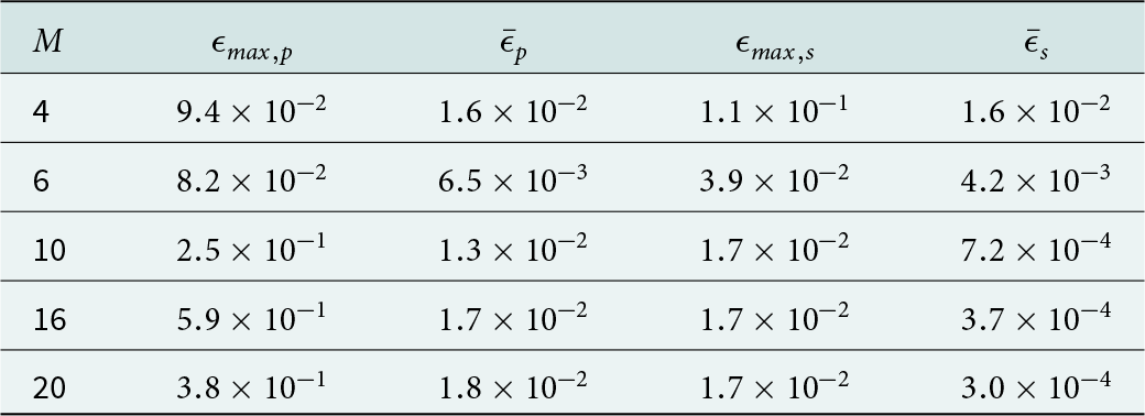
Diffraction: Interpolation accuracy versus number of interpolation points

Table 2 Long description
Columns list M, epsilon max p, mean epsilon p, epsilon max s, and mean epsilon s. For M 4, epsilon max p is 0.094 and mean epsilon p is 0.016; epsilon max s is 0.11 and mean epsilon s is 0.016. For M 6, epsilon max p is 0.082 and mean epsilon p is 0.0065; epsilon max s is 0.039 and mean epsilon s is 0.0042. For M 10, epsilon max p is 0.25 and mean epsilon p is 0.013; epsilon max s is 0.017 and mean epsilon s is 0.00072. For M 16, epsilon max p is 0.59 and mean epsilon p is 0.017; epsilon max s is 0.017 and mean epsilon s is 0.00037. For M 20, epsilon max p is 0.38 and mean epsilon p is 0.018; epsilon max s is 0.017 and mean epsilon s is 0.00030.
We now examine the same scenario from the perspective of interpolating diffracted fields. In the case of polynomial interpolation, four distinct models are required. Two regions are identified within which to create polynomials that model diffraction from the vertical edge at  $(50,10,z)$. These regions comprise the trajectory both before and after the shadow boundary at
 $s=18$. Similarly, two regions are identified within which to create polynomials that model diffraction from the vertical edge at
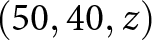 $(50,40,z)$. These regions correspond to the portion of the trajectory before and after the shadow boundary at
 $s=72$.
 $M$ interpolation points are used in each of the four regions. In each case, exact data at these points is used to make a single polynomial of degree
 $M-1$ in this region or a cubic spline interpolation across
 $M-1$ subregions. In all cases, a ray trace is required for each of the
 $M$ interpolation points. In the case of cubic spline interpolation, a further two ray traces are required, one at the start and end of the interpolation regions, in order to numerically estimate the derivative of the slowly varying field quantities at these end points. Hence, for this example,
 $4M$ ray traces are needed for polynomial interpolation along the entire trajectory while
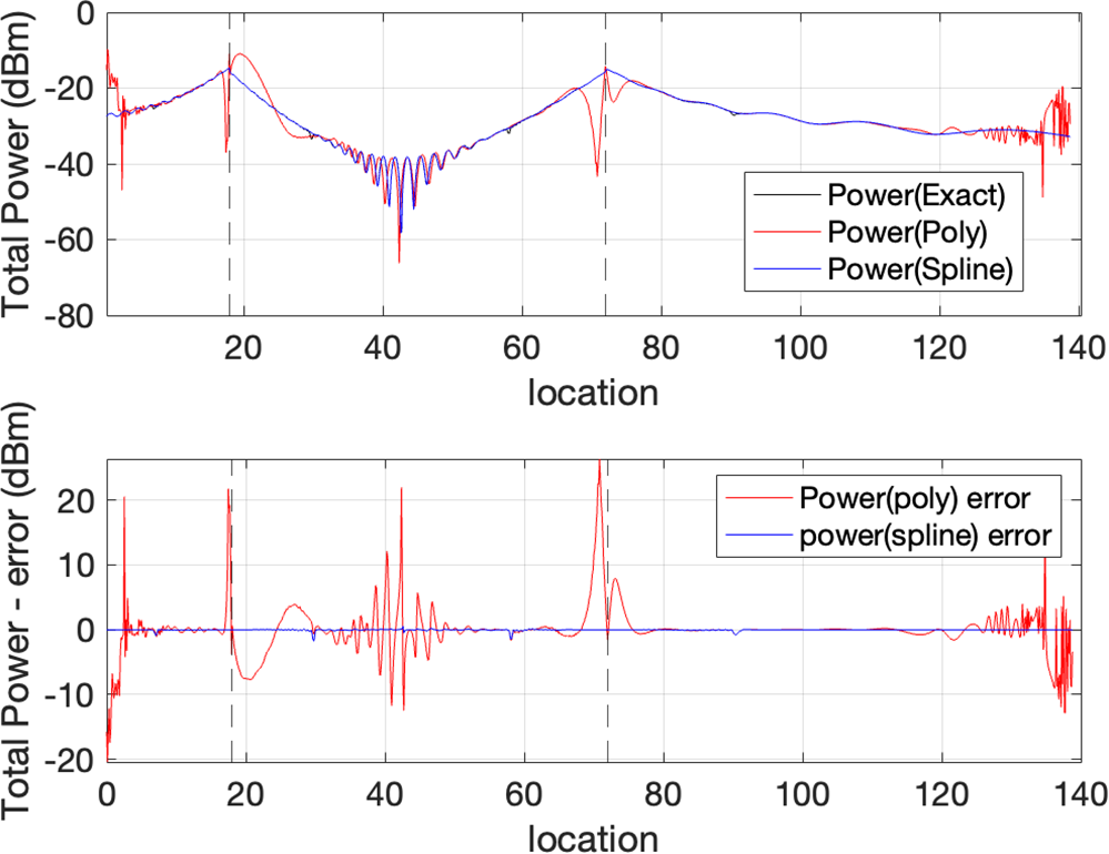
 $4 \left(M+2 \right) = 4M + 8$ ray traces are needed for cubic spline interpolation. The error is again defined as per Equation (16). Referring to Table 2 it is noted that cubic spline offers a more stable interpolation method in this instance. This is due to the relatively rapid variations of the interpolated quantities in the vicinity of the shadow boundaries. Polynomial interpolation can fit the sampled data but is subject to very rapid oscillation at intermediate points as
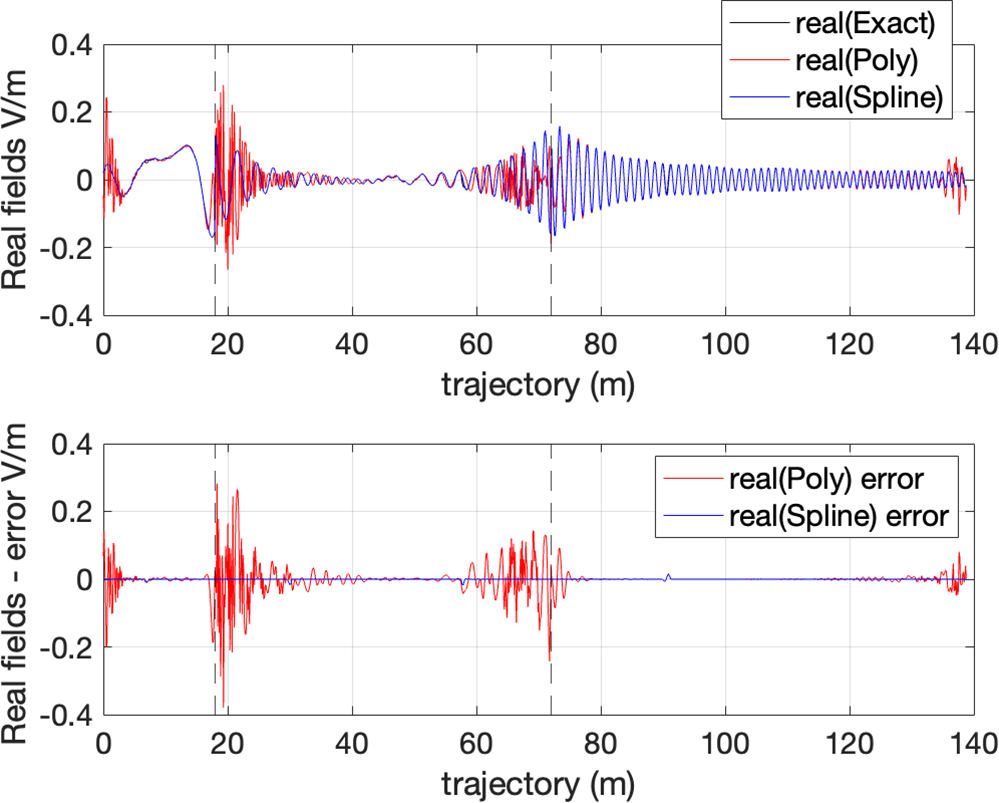
 $M$ grows. In contrast, cubic splines offer sufficient flexibility to model the fields within each sub-domain but are low order and do not introduce instabilities at non-sampled points. This is illustrated in Figures 6 and 7, which respectively show the absolute value of the diffracted field and the real value of the diffracted field along the receiver trajectory for the case of
 $M=16$. Note the rapid oscillations in the fields in the vicinity of the shadow boundaries when polynomial interpolation is employed. In contrast, the fields produced by cubic splines are stable throughout the region and offer excellent agreement with the exact values. Figure 7 shows the real-valued fields for this same example. Again, the cubic spline is able to accurately model the fields near the shadow boundaries as well as their phase evolution along the route.
Top: Exact and approximated diffracted fields along a portion of the trajectory for the validation example. Black curve is the exact power associated with the  $z$ component of the electric field. Red and blue are
 $M=20$ polynomial and cubic spline interpolated approximations (the latter effectively overlaying the exact values). Bottom: Error between exact and interpolated fields. Red is the error associated with the polynomial, while blue is the error given by the cubic spline approximation. Black vertical dotted lines indicate the location of the shadow boundaries.

Top: Exact and approximated diffracted fields along a portion of the trajectory for the validation example. Black curve is the real value of the exact  $z$ component of the electric field. Red and blue are polynomial and cubic spline interpolated approximations (the latter effectively overlaying the exact values). Bottom: Error between exact and interpolated fields. Red is the error associated with the polynomial, while blue is the error given by the cubic spline approximation. The dotted vertical lines denote the position of the shadow boundaries.

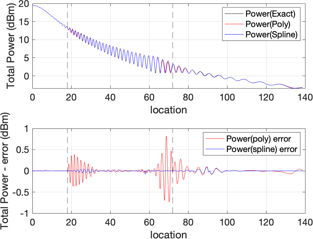
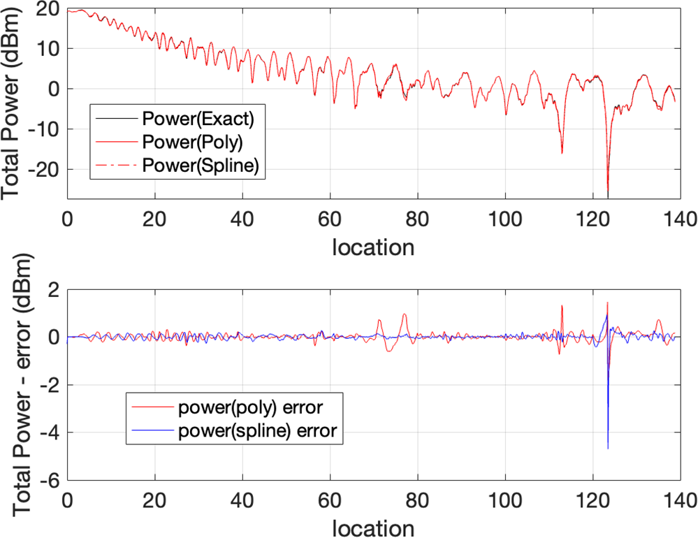
Finally, Figure 8 shows the total fields (incident plus reflected plus diffracted rays) along the entire trajectory. Exact fields are shown along with interpolated fields for the case  $M=8$. The superior performance of the cubic spline interpolation is evident in the lower plot, which shows the error in the approximated fields along the route. The cubic spline interpolation essentially overlays the exact result.
Total power along validation route. Top plot shows exact power and two interpolated approximations. Bottom plot shows error in polynomial approximation (red) and spline approximation (blue).

Geometry for error bound analysis.

Error bounds and sampling requirements
The use of cubic splines allows a rudimentary level of error analysis to be performed. In particular, it is shown in [Reference Hall and Meyer16] that if a function  $f$ is approximated using a cubic spline
 $p$ based on equi-spaced samples a distance
 $h$ apart, the maximum error is bounded as follows
 \begin{equation}
\| f - p \|_\infty \leq C_0 \| f^{(4)} \|_\infty h^4
\end{equation}
with  $C_0 = \frac{5}{384}$ and
 $f^{(4)}$ the fourth derivative of
 $f$. The validity of this bound is explored below.
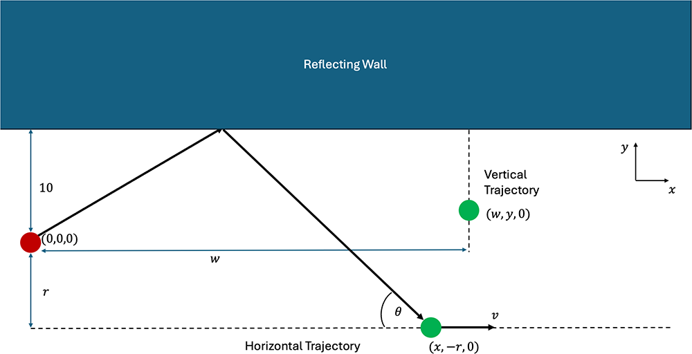
Consider the situation in Figure 9. A vertical dipole is placed at  $(0,0,0)$,
 $10m$ from a reflecting wall (
 $\epsilon_r = 4$). It radiates at
 $6GHz$. The fields associated with the reflected ray will be examined along horizontal (parallel to the wall) and vertical (perpendicular to the wall) trajectories. The horizontal trajectory runs from
 $(0,-r,0)$ to
 $(100,-r,0)$, while the vertical trajectory is shorter and runs from
 $(w,0,0)$ to
 $(w,9,0)$. In each case, 10 sample points are chosen along the trajectory in order to create data to make the approximation. This means that the sampling distance
 $h$ is equal to 11.11 m and 1 m in the horizontal and vertical trajectories, respectively.
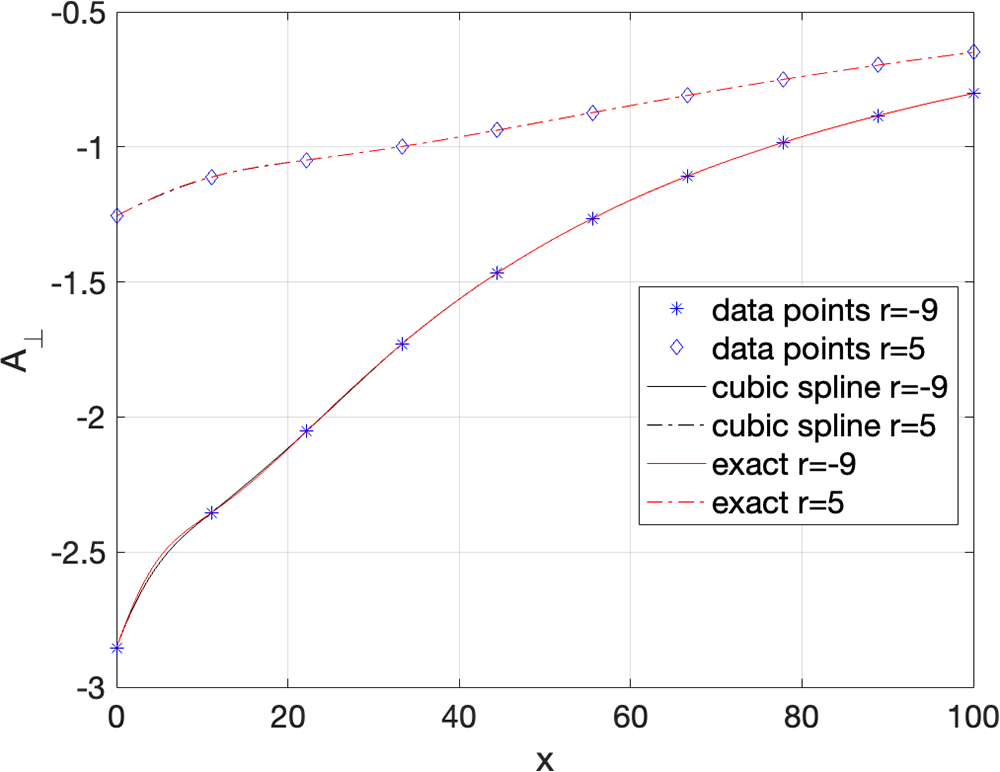
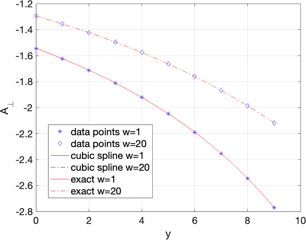
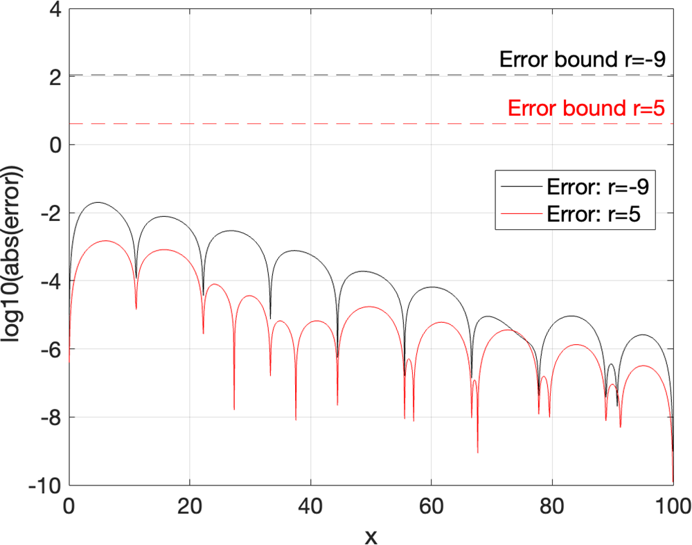
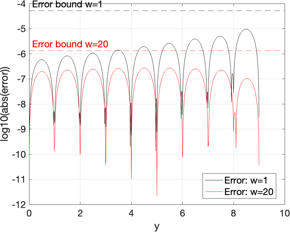
Figures 10 and 11 show  $A_\perp$ and its cubic spline approximation for both the horizontal and vertical trajectories, respectively. A high level of agreement can be noted, with the exact and interpolated values essentially overlapping. A better sense of the accuracy can be obtained from Figures 12 and 13, which show the error between the exact
 $A_\perp$ and its interpolated value (on a log scale) along the horizontal and vertical trajectories, respectively. The error bound (Equation (17)) is included in each case for reference. It is seen that the error is indeed bounded by the theoretical bound in each case. As can perhaps be expected, the error is largest for points where the reflection coefficient is changing most rapidly (i.e. in Figure 12 when
 $r=-9$ and the points are near the wall). Note that the fourth derivative information,
 $\| f^{(4)} \|_{\infty}$, needed to compute the bound was explicitly computed for this purely illustrative example.
 $A_\perp$ associated with the reflected ray computed along two horizontal trajectories from
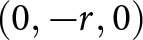 $(0,-r,0)$ to
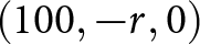 $(100,-r,0)$ (for
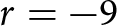 $r=-9$ and
 $r=5$) 10 data points are used in each case to make the cubic spline interpolated approximation.

 $A_\perp$ associated with the reflected ray computed along two vertical trajectories from
 $(w,0,0)$ to
 $(w,9,0)$. 10 data points are used in each case to make the cubic spline interpolated approximation.

Error between exact and approximate values of  $A_\perp$ as plotted in Figure 10. Black curve shows the error for
 $r=-9$, while red shows the error for
 $r=5$. Error bounds (Equation (17)) included for reference.

Error between exact and approximate values of  $A_\perp$ as plotted in Figure 11. Black curve shows error for
 $w=1$ while red shows error for
 $w=20$. Error bounds (Equation (17)) included for reference.

This analysis can be applied to other physical quantities associated with an interpolated ray. Assuming a receiver moving at  $v$ ms
 $^{-1}$ along the horizontal trajectory depicted in Figure 9, one can compute the Doppler shift associated with the reflected ray as
 \begin{equation}
f_D = \frac{v}{\lambda} \cos \theta
\end{equation}
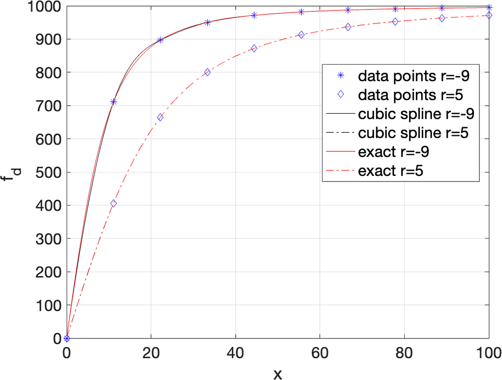
Figure 14 shows the Doppler shift associated with this multipath component, computed exactly and one based on cubic spline interpolation for the case where  $v =50$ms
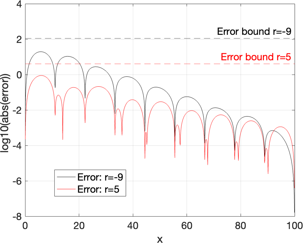
 $^{-1}$. The errors are shown in Figure 15 along with the error bounds.
Doppler shift experienced by receiver traveling at 50 ms $^{-1}$ along horizontal trajectories depicted in Figure 9. Cubic spline interpolation based on 10 sampled values along the trajectory.

Errors and error bounds for Doppler shift example.

It can be seen that the bound given by Equation (17) represents a usefully tight bound on the error. In particular, Equation (17) can be rearranged to express the sampling spacing required to achieve a desired accuracy. In particular, if the error is to be no greater than  $\epsilon$ along a path, then
 $h$ must satisfy
 \begin{equation}
h \leq \left( \frac{\epsilon}{C_0 \| f^{(4)} \|_\infty } \right)^{\frac{1}{4}}
\end{equation}
Clearly, the slower the variation of the function (as measured by the maximum value of its fourth derivative), the fewer interpolation points are necessary to achieve a specified accuracy. This bound is thus a useful starting point to develop practical guidelines on the level of field sampling necessary to reliably implement the interpolation. However, it does require knowledge of the fourth derivative of the quantity to be approximated. This was computed exactly for these illustrative examples but will need to be reliably estimated if this analysis is to support practical implementation. This will be a focus of future work.
Results
In this section, the performance of the interpolation schemes is examined in the context of propagation in a street canyon comprising eight buildings (Figure 16) and a transmitter radiating at 300 MHz. A receiver travels for 10 s at a speed of 50 km/h along the indicated linear route, covering a distance of total of just under 140 m. It enters and exits multiple lit regions corresponding to multiple higher-order rays as it travels. The field is calculated at 1200 locations along the trajectory, and up to 2 reflections/diffractions were allowed, using the DCU in-house ray tracer previously developed in the context of references [Reference Hussain and Brennan6], [Reference Hussain and Brennan7], and [Reference Hussain and Brennan11]. The reference solution involved an exact ray trace at each location and required the computation of 62,183 rays, which took 590 s with an Apple M4 processor. To create the approximate model, suitable  $M$ was set to 6 for each lit region. Fields were approximated using the concepts in Sections “Interpolation of reflected rays” and “Interpolation of diffracted rays.” For polynomial interpolation, this meant that fifth-order polynomials were created. This required the explicit computation of 3858 rays, and the total process took 3.5 s, a saving of 99.5%. For cubic spline interpolation, this meant that each lit region was divided into 5 sub-domains. This required the explicit calculation of 5144 rays and took 4.8 s, a saving of roughly 99.2%.
Street-canyon geometry.

Figure 17 depicts how the power delay varies with time (horizontal axis) as the receiver moves along the trajectory. It was computed using exact RT. Each curve represents the contribution caused by a single ray (multipath component) and its color denotes the power associated with that component. The lowest curve denotes the incident field via direct line of sight, while all other curves represent some higher-order combination of reflected/diffracted rays. Figure 18 shows the same information computed using the cubic spline interpolation. Finally, the total narrow band fields along the route are depicted in Figure 19. Both interpolated results show excellent agreement with the exact values.
Exact time-varying power delays along receiver route.

Figure 17 Long description
Exact Power Delay. The horizontal axis is labeled, Time (s), with tick labels from 0 to 10. The vertical axis is labeled, Delay (microseconds), with tick labels from 0.0 to 0.8. A vertical color scale bar at the right is labeled, Power (dB), with tick labels at 0, minus 20, minus 40, minus 60, minus 80, minus 100 and minus 120. The plot contains many curved line traces across the time range. Several traces start near delay 0.0 microseconds at time 0 and rise toward higher delay values by time 10. Multiple traces form arcs that dip and then rise, with many traces converging and crossing between about time 7 to 10 and delay about 0.5 to 0.8 microseconds. A dense band of traces appears near the top of the plot between about delay 0.7 and 0.8 microseconds across much of the time range.
Approximate time-varying power delays along the receiver route using cubic spline interpolation.

Figure 18 Long description
The graph is titled Approximate Power Delays. The horizontal axis is labeled Time in seconds, ranging from 0 to 10 in increments of 1. The vertical axis is labeled Tau in seconds, ranging from 0 to 0.8 in increments of 0.1. A color gradient scale on the right side of the graph indicates power in decibels, ranging from 0 at the top to minus 80 at the bottom. Many individual lines are plotted across the graph, each representing a separate power delay realization. The lines are not individually labeled in the graph. Each line carries a distinct position along the color gradient scale, reflecting its associated power level in decibels. The lines are not uniformly distributed. Several lines are clustered near the lower portion of the vertical axis, between Tau values of approximately 0 to 0.2 seconds, throughout most of the time range. A smaller number of lines occupy the mid to upper range of the vertical axis, between Tau values of approximately 0.4 to 0.8 seconds. The highest Tau values, near 0.8 seconds, are reached by only a few lines and are most visible between Time values of approximately 2 and 8 seconds. Lines in the lower Tau range remain relatively stable across the full time span from 0 to 10 seconds. Lines in the upper Tau range show more variation, with some rising and others shifting across the time span. The overall distribution of lines spans the full vertical range from near 0 to approximately 0.8 seconds, with the greatest density of lines concentrated in the lower Tau region across all time values.
Top: Total narrowband power along trajectory indicated in Figure 16. Bottom: Error between interpolated and exact power.

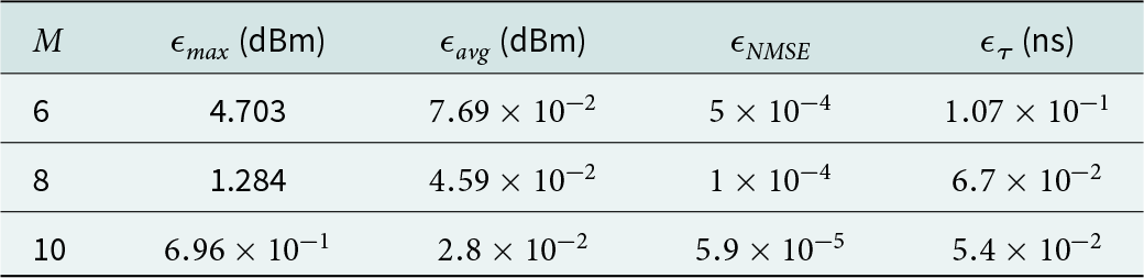
To examine the effect of interpolation accuracy on channel-level metrics, we computed various KPI for different values of  $M$. If
 $p_i$ is the exact received power at location
 $i$ and
 $\tilde{p}_i$ is the interpolated value, we define the maximum, average, and normalized mean square errors as
 \begin{eqnarray*}
\epsilon_{max} & = & \max_i \left| p_i - \tilde{p}_i \right| \\
\epsilon_{avg} & = & \frac{1}{N} \sum_{i=1}^N \left| p_i - \tilde{p}_i \right| \\
\epsilon_{NMS} & = & \frac{\sum_{i=1}^N \left( p_i - \tilde{p}_i \right)^2 }{\sum_{i=1}^N p_i^2 }
\end{eqnarray*}
We also compute the RMS delay spread  $\tau_i$ at each location as well as its value based on cubic spline interpolation
 $\tilde{\tau}_i$. We define the average RMS delay spread error as
 \begin{equation*}
\epsilon_\tau = \frac{1}{N} \sum_{i=1}^N \left| \tau_i - \tilde{\tau}_i \right|
\end{equation*}
Table 3 shows how these values vary for the trajectory in Figure 16 for various values of  $M$ using cubic spline interpolation.
Channel metric errors for various values of  $M$

Table 3 Long description
Channel error metrics are listed for three values of M, with columns for epsilon max in dBm, epsilon avg in dBm, epsilon NMSE, and epsilon tau in nanoseconds. For M 6, epsilon max is 4.703 dBm, epsilon avg is 0.0769 dBm, epsilon NMSE is 0.0005, and epsilon tau is 0.107 ns. For M 8, epsilon max is 1.284 dBm, epsilon avg is 0.0459 dBm, epsilon NMSE is 0.0001, and epsilon tau is 0.067 ns. For M 10, epsilon max is 0.696 dBm, epsilon avg is 0.028 dBm, epsilon NMSE is 0.000059, and epsilon tau is 0.054 ns. From M 6 to M 10, epsilon max, epsilon avg, epsilon NMSE, and epsilon tau each decrease.
Conclusion
This paper proposes a novel approximate method to compute reflected and diffracted fields along the trajectory of a moving receiver. The rapidly oscillating field associated with each ray is factorized into a product of terms, each of which can be modeled using a low-degree interpolation. Both polynomial interpolation and cubic spline interpolation are employed, and both are shown to be effective in accurately modeling field behavior within the corresponding lit region. However, cubic spline interpolation is shown to be more stable as the degree of interpolation is raised in order to increase accuracy. Results demonstrate good agreement for examples involving a single reflecting face and a street canyon. Results were provided showing excellent agreement for both field strength and channel delay. Future work will extend the method to the case of a moving TX/RX pair. In addition, we intend to extend the ideas to the problem of diffuse scattering, whereby field contributions are collected from a grid of patches on each face. The geometric quantities underpinning diffuse scattering vary slowly, thereby making it a candidate for the approach outlined in this paper.
Competing interests
The authors declare none.

Conor Brennan received a B.A. (Mod) in Mathematics and a PhD from Dublin University (Trinity College) in 1994 and 1998, respectively. He joined the School of Electronic Engineering, Dublin City University in 2003, where he is a Professor. He has served as the Irish Representative on multiple COST Actions in the area of wireless communications and is a teacher on the European School of Antennas and Propagation. In 2026, he was the General Chair of the European Conference on Antennas and Propagation (EuCAP26). He has authored more than 100 peer-reviewed publications in international journals and conference proceedings. His current research interests include wireless communications and computational methods for electromagnetic wave scattering and propagation. Dr. Brennan is an Associate Editor of IEEE Transactions on Antennas and Propagation.

Allan Wainaina Mbugua received the B.Sc. degree in telecommunication and information engineering from the Jomo Kenyatta University of Agriculture and Technology, Juja, Kenya, in 2014; the M.Sc. degree in telecommunications engineering from the University of Cassino and Southern Lazio, Cassino, Italy, in 2018; and the Ph.D. degree from Aalborg University, Aalborg, Denmark, in 2023. He is currently working as a Senior Engineer with Huawei Technologies Duesseldorf GmbH, Munich, Germany. His current research interests include radio channel sounding, radio channel simulation, and radio channel emulation.

Dr. Yun Chen received the B.Sc. from the University of Duisburg-Essen, Germany, in 2006, the M.Sc. degree from the University of Duisburg-Essen, Germany, in 2008, and the Ph.D. degree from the University of Duisburg-Essen, Germany, in 2012. He was with Rohde & Schwarz and Fraunhofer research society in Munich, Germany, and is currently working as a team manager with Huawei Technologies Duesseldorf GmbH, Munich, Germany, with a research focus on 5G, WiFi, and smart home systems testing and simulations.

Sajjad Hussain received the B.Sc. degree in electrical engineering from the University of Engineering and Technology at Taxila, Taxila, Pakistan, in 2006, the M.Sc. degree in telecommunications engineering from the University of Liverpool, Liverpool, UK, in 2008, and the Ph.D. degree in electronic engineering from Dublin City University, Dublin, Ireland, in 2017. From 2009 to 2013, he was a Technical and Test Engineer with Vodafone Automotive Ltd., Manchester, UK. He is currently an Assistant Professor with the School of Electrical Engineering and Computer Sciences, National University of Sciences and Technology, Islamabad, Pakistan. His research interests include radio channel modeling for future radio networks using RT and machine learning.






















 Open access

