2 An increasingly meandering signature with distance from the wall

Throughout this paper $x$ , $y$ and $z$ refer to the streamwise, spanwise and wall-normal directions, with $u$ , $v$ and $w$ indicating the respective total velocity components.

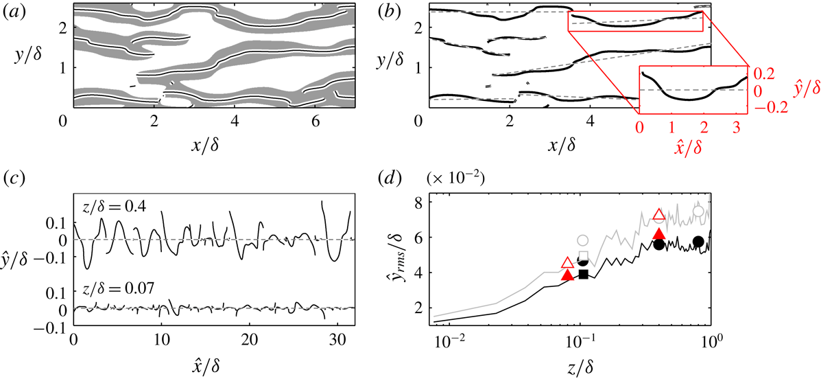
We first quantify how the large low-momentum regions become increasingly wavy with distance from the wall. In figure 2(a), the grey-shaded regions indicate the filtered signature of $u_{f}^{\prime }<0$ (subscript $f$ denotes filtered quantity) for the example shown in figure 1(b). For this wall height ( $z/\unicode[STIX]{x1D6FF}=0.4$ ), we apply a 2D Gaussian filter ( $\unicode[STIX]{x1D70E}=2$ ) with the size of $2.1\times 0.43\unicode[STIX]{x1D6FF}$ in the $x\times y$ direction. This filter size corresponds to the length and width of the correlation function $R_{u^{\prime }u^{\prime }}=0.15$ , hence it is a function of wall height. Note that the change in $R_{u^{\prime }u^{\prime }}$ dimension (i.e. our filter size) with wall height is well documented in the literature (Tomkins & Adrian Reference Tomkins and Adrian2003; Ganapathisubramani et al. Reference Ganapathisubramani, Hutchins, Hambleton, Longmire and Marusic2005; Lee & Sung Reference Lee and Sung2011; Sillero et al. Reference Sillero, Jiménez and Moser2014). From this filtered field, we can identify the ‘spine’ of each low-momentum region by finding the local minima of $\unicode[STIX]{x2202}u/\unicode[STIX]{x2202}y=0$ at every streamwise position, in a similar approach to that followed by Schoppa & Hussain (Reference Schoppa and Hussain2002). To gauge the meandering behaviour, we quantify the ‘waviness’ of these spines and employ it as a metric. In this manner, the width of the structure does not play any role in the quantification. In figure 2(b), the dashed line plotted over each spine indicates its linear fit. Accordingly, we treat these spines as fluctuation signals ${\hat{y}}$ about the fitted line (see inset). This also means that the linear orientation of the spines will not be considered. The concatenated ‘spine signals’ are displayed in figure 2(c), where we compare the projected signals for $z/\unicode[STIX]{x1D6FF}=0.07$ and 0.4.

Figure 2.

(a) Grey regions: $u_{f}^{\prime }<0$ at $z/\unicode[STIX]{x1D6FF}=0.4$ , highlighting the spine of each region. (b) Dotted line: the linear fit of each spine. Inset shows $\hat{x}$ , the projected linear fit to the streamwise direction; ${\hat{y}}$ : the projected spine about the linear fit. (c) The concatenation of the spines about their individual fitted line. (d) The meandering root mean square as a function of wall height. Lines: dataset of Sillero et al. (Reference Sillero, Jiménez and Moser2014); squares: smooth-wall data of Kevin et al. (Reference Monty and Hutchins2019); circles: de Silva et al. (Reference de Silva, Baidya, Hutchins and Marusic2018). Black line and closed symbols: cases where spines are longer than the filter size. Grey line and open symbols: cases where spines are longer than twice the filter size. Triangles: artificially generated streaks over herringbone riblets (Kevin et al. Reference Monty and Hutchins2019).

We can now compute the root mean square of these signals for multiple wall heights, and the trend is shown in figure 2(d). Note that we only consider the individual spine that is longer than the filter size, where the results are shown by the black line and closed symbols. Clearly this metric ( ${\hat{y}}_{rms}$ ) indicates that the spine of low-momentum regions increasingly fluctuates with wall distance, and the trend is consistent across numerical and experimental datasets. It is noted that the meandering amplitude flattens for $z/\unicode[STIX]{x1D6FF}>0.5$ . This is partly because the detected structures become shorter/patchier in the turbulent-intermittent region, which will bias the meandering detection (i.e will limit ${\hat{y}}_{rms}$ ). As a check, when we consider only those spines that are longer than twice the filter size (denoted by the grey line and open symbols), the overall meandering magnitude increases and we observe less flattening away from the wall. It is important to note that here we simply aim to demonstrate statistically that large-scale turbulence becomes increasingly wavy with wall distance, without putting emphasis on the exact rate of the increase.

Finally, the triangle symbols in figure 2(d) indicate the meandering magnitude of the artificially generated streaks studied by Kevin et al. (Reference Monty and Hutchins2019) in a spanwise-heterogeneous boundary layer (where the global or spanwise-averaged $\unicode[STIX]{x1D6FF}$ is used to normalise), and the results closely conform to the increasing trend of the canonical case. This observation suggests that the pronounced undulating behaviour, that in Kevin et al. (Reference Monty and Hutchins2019) was attributed to the imposed turbulent secondary flows, is in fact an underlying characteristic of large-scale turbulence structures.

2.1 Severely meandering turbulent signature at the edge of the boundary layer

Sillero et al. (Reference Sillero, Jiménez and Moser2014) reported that the spanwise-velocity component exhibits a large oblique/diagonal coherence. The $\pm 45^{\circ }$ (from streamwise axis) pattern is particularly discernible in the outermost part of the boundary layer. The coherence emerges statistically (e.g. in 2D correlation), if one decomposes by either the positive or negative spanwise-velocity sign. Thus far, little physical interpretation has been given to this phenomenon. de Silva et al. (Reference de Silva, Baidya, Hutchins and Marusic2018) described this occurrence as the spanwise-velocity signature of the arched head of a hairpin-type eddy. Indeed, when one considers the positive or negative spanwise velocity on a wall-parallel slice close to the head of a hairpin eddy, the imprints are diagonally positioned. Note that in making this observation, de Silva et al. (Reference de Silva, Baidya, Hutchins and Marusic2018) did observe that, in reality the obliqueness may involve ‘a range of representative eddies which are not necessarily forced to be streamwise aligned or symmetric’. In this spirit, we build on these previous observations of this unique oblique turbulent pattern.

Figure 3.

Example of (a) streamwise-velocity and (b) spanwise-velocity field at $z=\unicode[STIX]{x1D6FF}_{99}$ , highlighting several oblique $v$ features. Taken from dataset of Sillero et al. (Reference Sillero, Jiménez and Moser2014). Square insets highlight particular inclined features that are magnified in the following subfigures. (c–e) Vectors of velocity fluctuations, with contour of signed swirling strength $\unicode[STIX]{x1D706}_{ci}$ superimposed. Grey contour lines show $v^{+}=0.3$ in (b,c) and $v^{+}=-0.3$ in (d).

Figure 3(a,b) shows an instance of streamwise and spanwise velocity at $z=\unicode[STIX]{x1D6FF}_{99}$ at a different instance to that shown in figures 1 and 2. This snapshot is selected since it effectively highlights the oblique $v$ pattern as discussed by Sillero et al. (Reference Sillero, Jiménez and Moser2014) and de Silva et al. (Reference de Silva, Baidya, Hutchins and Marusic2018). When carefully examining many vector fields around similar oblique features, such as in figure 3(c–e), we observed that the low-speed (streamwise negative) fluctuations associated with vortex groups, which are typically more streamwise aligned, are now consistently oriented at approximately $\pm 45^{\circ }$ . This is further illustrated by the compact swirling-strength contours, $\unicode[STIX]{x1D706}_{ci}$ (computed using the method described in Adrian, Christensen & Liu (Reference Adrian, Christensen and Liu2000a )), which indicate the presence of wall-normal vortices in figure 3(c–e). Note that in these figures they appear to be roughly aligned along the diagonals. Based on these simple observations, we surmise that the negative $u^{\prime }$ fluctuations associated with vortex packets (Adrian et al. Reference Adrian, Meinhart and Tomkins2000b ) or clusters (del Álamo et al. Reference del Álamo, Jiménez, Zandonade and Moser2006), which themselves are often yawed or appear oblique in the outer region, are resolved or decomposed in the $y$ -direction as these oblique $v$ features. Not only does this observation provide an extension to the work of Sillero et al. (Reference Sillero, Jiménez and Moser2014) and de Silva et al. (Reference de Silva, Baidya, Hutchins and Marusic2018) regarding the emergence of these oblique patterns in $v$ , it also further demonstrates that turbulent events become increasingly misaligned from the main-flow direction with wall height. As a final point, the lesser degree of meandering at lower wall heights further explains why the apparent $v$ diagonals are less oblique closer to the wall at much smaller angles than $\pm 45^{\circ }$ . This behaviour was also observed by de Silva et al. (Reference de Silva, Baidya, Hutchins and Marusic2018) in the log region, though at the time an explanation for this observation was still lacking.

3 Outer-layer periodicity of the large structures

In a spanwise-heterogeneous boundary layer (viz. over herringbone roughness), where the large-scale low-momentum regions were forcibly formed at fixed spanwise locations, Kevin et al. (Reference Monty and Hutchins2019) observed a dominant streamwise-repeating behaviour of those low-momentum structures. This outer-layer pattern emerged in the correlation-coefficient map, $R_{u^{\prime }u^{\prime }}$ , when it was computed at a spanwise reference location midway between where the low- and high-momentum regions were induced. In spanwise-homogeneous (smooth-wall) boundary layers however, where these turbulent regions occur spatially and temporally at random, extracting such repeating patterns becomes less straightforward.

Figure 4.

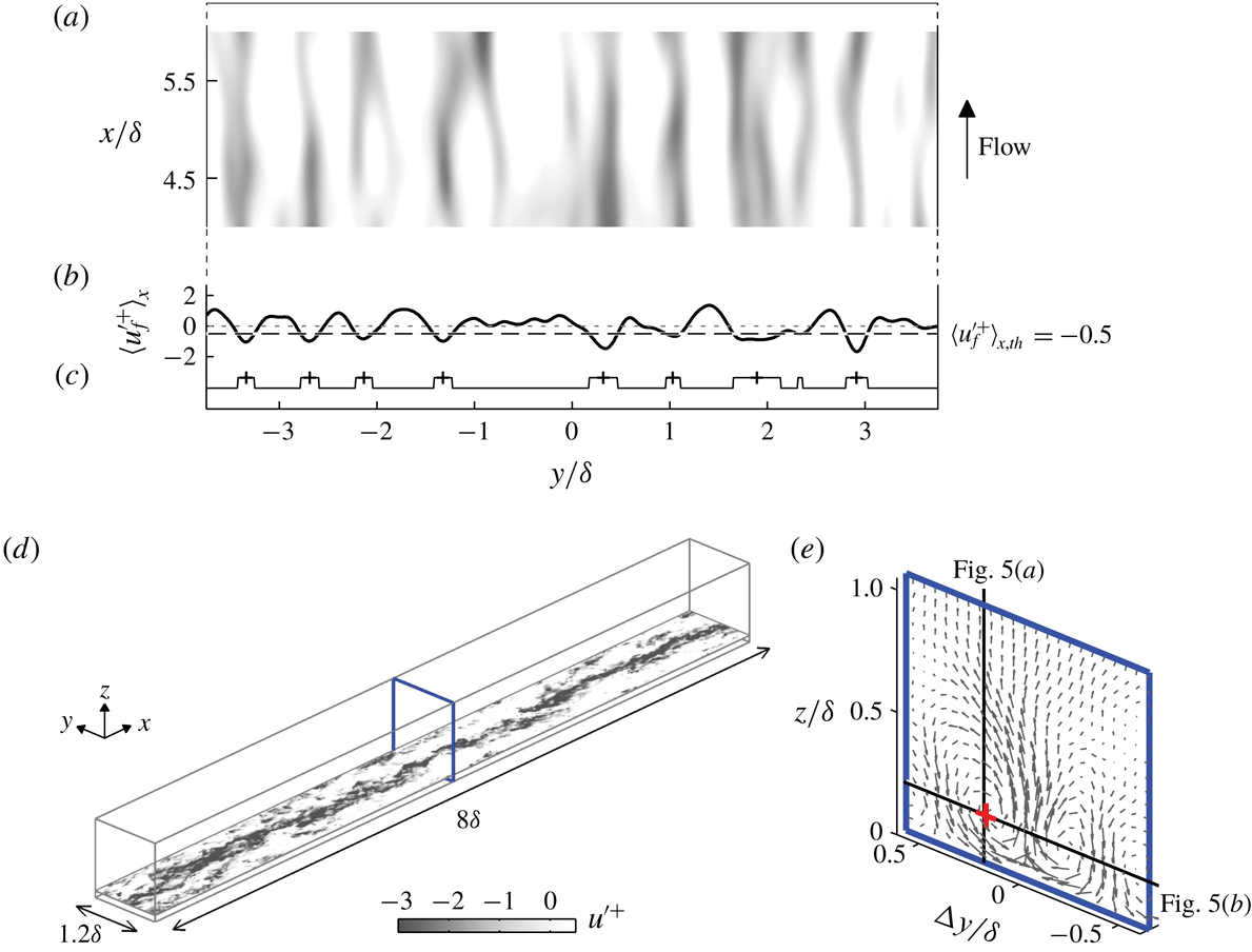
Detection of low-speed streaks from the dataset of Sillero et al. (Reference Sillero, Jiménez and Moser2014). (a) A wall-parallel (top-view) snapshot, showing filtered velocity $u_{f}^{\prime }$ at $z/\unicode[STIX]{x1D6FF}=0.07$ . Only a subset of the extracted data is plotted from a total of $8\unicode[STIX]{x1D6FF}$ streamwise domain. (b) Distribution of streamwise-averaged velocity within the entire $8\unicode[STIX]{x1D6FF}$ -long domain, $\langle u_{f}^{\prime }\rangle _{x}$ . (c) A logic signal for the condition $\langle u_{f}^{\prime }\rangle _{x}<-0.5$ . The $+$ symbols show the spanwise centre of the detected streaks. (d) An example wall-parallel slice of streamwise-velocity fluctuations at $z/\unicode[STIX]{x1D6FF}=0.07$ corresponding to one of the detected streaks, showing a continuous long low-momentum region within the narrow extracted domain. (e) The ensemble-averaged $V$ and $W$ vectors on the cross-plane marked in (d). Here $\unicode[STIX]{x0394}y=0$ indicates the centre of the extracted domain. The $+$ (red) symbol indicates the reference point $(\unicode[STIX]{x0394}y_{ref},z_{ref})/\unicode[STIX]{x1D6FF}=(0.2,0.2)$ where the correlation maps shown later in figure 5 are computed, and the black lines illustrates the corresponding vertical and horizontal planes.

3.2 Spatial statistics in the outer layer

As a conjecture, we associate the collection of streaks in smooth-wall boundary layers (identified above) and the accompanying roll-modes shown in figure 4(e), to the continuous low-momentum regions that occur in spanwise-heterogeneous layers and the associated ‘mean secondary flows/roll-modes’. Hence, we will replicate the analysis of Kevin et al. (Reference Monty and Hutchins2019) for spanwise-heterogeneous layers, in order to extract the possible streamwise-repeating behaviour from the canonical smooth-wall flows. We first compute the correlation coefficient $R_{u^{\prime }u^{\prime }}$ at a spanwise position corresponding to the midpoint between the upwash- and downwash-flow regions. An analysis of figure 4(e) reveals that this point occurs at approximately $(\unicode[STIX]{x0394}y_{ref},z_{ref})/\unicode[STIX]{x1D6FF}=(0.2,0.2)$ , as shown by the $+$ (red) symbol in figure 4(e). The correlation $R_{u^{\prime }u^{\prime }}$ is calculated on the vertical and horizontal planes indicated by the solid lines in this figure. The reasoning behind selecting $\unicode[STIX]{x0394}y_{ref}/\unicode[STIX]{x1D6FF}=0.2$ is that, at this spanwise location (i.e. the crossover between low-momentum/upwash and high-momentum/downwash regions), any meandering will lead to pronounced periodic fluctuations between positive and negative $u^{\prime }$ .

Figure 5.

Maps of two-point correlation function $R_{u^{\prime }u^{\prime }}$ in the (a) $xz$ - and (b) $xy$ -planes about $(\unicode[STIX]{x0394}y_{ref},z_{ref})/\unicode[STIX]{x1D6FF}=(0.2,0.2)$ . The $+$ (red) symbols show the reference location. This reference position is also indicated in figure 4(e). Black contours lines: positive levels of 0.05, 0.15 and 0.3; blue contours lines: negative levels of $-0.05$ and $-0.1$ . Grey contours on (a) show the contours of standard (streamwise- and spanwise-ensembled) two-point correlation with contour levels of 0.05 and 0.3. Dot-dashed planes indicate the middle of the domain, $\unicode[STIX]{x0394}y=0$ plane.

Figure 5(a) displays the resulting correlation map in the streamwise/vertical plane. The reference height $z_{ref}/\unicode[STIX]{x1D6FF}=0.2$ corresponds to the centre of the mean roll-modes following Kevin et al. (Reference Monty and Hutchins2019), and we emphasise that changing the reference height within the outer layer has little effect on the present conclusions. Clearly the $R_{u^{\prime }u^{\prime }}$ map constructed in this manner differs substantially from the standard correlation map at the same reference height $z_{ref}/\unicode[STIX]{x1D6FF}$ (shown by grey filled contours in figure 5 a), particularly for the larger-size coherence. When ensembled in this way, at a certain distance to the span of a detected large-scale event, a clear streamwise-repeating behaviour of positive and negative correlations manifests which would ordinarily be masked by the spanwise-averaging process of a standard two-point correlation. Note that when the correlation is computed about the upwash- and downwash-flow region, i.e. $y/\unicode[STIX]{x1D6FF}=0$ and 0.45 in figure 4(e), the repeating pattern is not evident (not shown here for brevity). Figure 5(b) displays this alternating coherence in the wall-parallel slice, where again we see strong signs of streamwise periodicity (with streamwise alternating regions of positive and negative correlation) and a close resemblance to the behaviour observed in spanwise-heterogeneous boundary layers (Kevin et al. Reference Monty and Hutchins2019).

Various interpretations can be drawn when observing an alternating sign of statistical pattern such as those shown in figure 5. Elsinga et al. (Reference Elsinga, Adrian, Van Oudheusden and Scarano2010) proposed the idea of larger vortex organisation where large-scale (mostly symmetrical) hairpin structures are arranged in an alternating configuration. However, as established previously, the outer-layer behaviour observed here is characterised by events with a much longer streamwise extent than would be implied from this interpretation. The more likely explanation based on the observations of figures 1 and 2, is simply that this periodicity is a result of meandering. This observation was concluded in spanwise-heterogeneous flows by Kevin et al. (Reference Monty and Hutchins2019) using a conditional analysis, where the meandering bend/turn is shown to be associated with a non-symmetrical wall-normal vortex structure.

4 A closer look at the representative streamwise roll-modes

In the conditionally averaged view, a pair of counter-rotating streamwise vortices, as represented in figure 4(e), are known to flank the large-scale turbulence structures (Hutchins, Hambleton & Marusic Reference Hutchins, Hambleton and Marusic2005; del Álamo et al. Reference del Álamo, Jiménez, Zandonade and Moser2006; Dennis & Nickels Reference Dennis and Nickels2011). In spanwise-heterogeneous wall flows, where the high- and low-momentum regions are spatially locked at fixed locations in the spanwise direction, these flanking vortices are readily apparent in the unconditional mean statistics as the counter-rotating ‘secondary flows/roll-modes’. Instantaneously, however, Kevin et al. (Reference Monty, Bai, Pathikonda, Nugroho, Barros, Christensen and Hutchins2017) found that these secondary roll-modes are more often constituted by one-sided streamwise vortices than two-sided/counter-rotating motions. Hence, they concluded that turbulent secondary flows, whose time-averaged magnitude is often weak, are an artefact arising from superposition of the more typical non-symmetrical vortices within the spanwise-heterogeneous boundary layers.

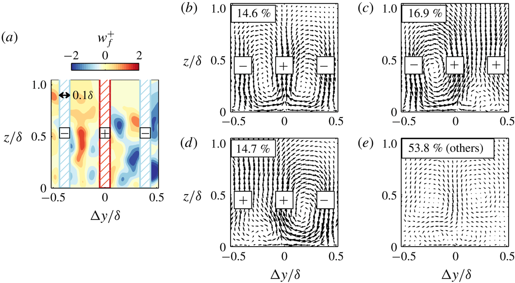
In this section, by employing a similar sorting technique to Kevin et al. (Reference Monty, Bai, Pathikonda, Nugroho, Barros, Christensen and Hutchins2017), though this time applied to a smooth-wall (spanwise-homogeneous) boundary layer dataset, we aim to assess the likelihood of instantaneous streamwise vortices appearing symmetrically or otherwise. The sorting method is based on the instantaneous vertical velocity at three spanwise locations about the centre of the identified low-speed streak as illustrated in figure 6(a). The instantaneous $w_{f}$ field is locally averaged within a spanwise width of $0.1\unicode[STIX]{x1D6FF}$ (within the hatched region on figure 6 a) to determine the main vertical-flow direction in these three detection locations. Note that these locations correspond to the upwash and downwash regions shown in figure 4(e). As an example, the combination result illustrated in figure 6(a) is ‘negative–positive–negative’ or ( $-,+,-$ ), which corresponds to a ‘down–up–down’ flow pattern. Thus, this particular instance represents a counter-rotating direction similar to figure 4(e). Note that there will be $2^{3}$ sign/pattern combinations. We can then sort all the cross-stream ( $yz$ ) slices along the detected structures identified in § 3.1, based on each combination. Accordingly, a conditionally averaged flow field can be produced for each pattern. If all combinations are included, we recover the generally accepted conditionally averaged vortices shown in figure 4(e).

Figure 6.

(a) An example of filtered wall-normal velocity field associated with large-scale low-momentum region. The hatched regions show the areas where $w_{f}$ is averaged to determine the common vertical-flow directions. (b) Conditionally averaged vectors when the averaged- $w_{f}$ is $-,+,-$ . (c,d) Conditional vectors when the averaged- $w_{f}$ is $-,+,+$ and $+,+,-$ . (e) Conditional vectors for the remaining combinations. Vector size is comparable between figures.

Figure 6(b) displays the conditionally averaged field when the combination is $-,+,-$ . As expected, counter-rotating vortices appear, resembling the typical quasi-streamwise counter-rotating rollers that on average border the turbulent events. Surprisingly, this pattern accounts for only 15 % of the instantaneous fields, while the large one-sided patterns, shown in figure 6(c,d), represent 32 %. Moreover, figure 6(e), which includes the other five combinations (i.e. $+,+,+$ ; $-,-,-$ ; $-,+,-$ ; $-,+,+$ ; $+,+,-$ ), where the individual result does not resemble the overall mean roll-modes, occupy the majority of the flow fields.

Although the exact fractions of each combination differs from the heterogeneous flow (Kevin et al. Reference Monty, Bai, Pathikonda, Nugroho, Barros, Christensen and Hutchins2017), the key observations are consistent. Large streamwise rollers related to the turbulence structures are predominantly one-sided and rarely resemble the counter-rotating view. Hence, the representative eddy (and its weakness in strength, see figure 4 e), are likely to be an artefact of the superposition of various turbulent events. Though statistically sound, the risk with allowing symmetrical representative eddies to dominate our interpretations (i.e packet models and attached eddy hypothesis) is that important dynamical processes can be obscured. For example, the meandering of the low-speed streaks and the one-side vortex structure is reminiscent of the streak-vortex model, as put forward by Jeong et al. (Reference Jeong, Hussain, Schoppa and Kim1997) in the near-wall region, and more recently described by Flores & Jiménez (Reference Flores and Jiménez2010) in the log layer. Certainly the current results indicate that the large-scale vortices occur intermittently in space, as suggested by the large number of instances along the structures, yielding a negligible contribution to the overall ensemble. These observations further support the conclusion of Lozano-Durán & Jiménez (Reference Lozano-Durán and Jiménez2012), where they stated that the spanwise arrangements of large high- and low-speed events, which are directly related to the vortical structure between them, are more likely to occur as pairs (hence yield one-sided rotational motion) instead of in symmetric trios. Lastly, we note that the percentages shown in figure 6 resemble the meandering probability inferred by Hutchins et al. (Reference Hutchins, Monty, Ganapathisubramani, Ng and Marusic2011), although their technique was limited to aggregating the contributions displayed here by figure 6(b,e) as the ‘non-meandering events’.

5 Summary and schematic interpretation

Inspired by our previous findings in spanwise-heterogeneous boundary layers (Kevin et al. Reference Monty, Bai, Pathikonda, Nugroho, Barros, Christensen and Hutchins2017, Reference Monty and Hutchins2019), here we underline the pronounced unsteady behaviour of large-scale structures in canonical boundary layers. The relevant discussions are summarised below:

1. (i) The wall-parallel signature of large-scale structures becomes significantly meandering away from the wall. This trend is quantified by the meandering amplitude of the spines of the structures at each wall location. At the edge of the boundary layer, the severely yawed turbulent regions give rise to the oblique/diagonal coherence in the spanwise velocity, which was previously documented by Sillero et al. (Reference Sillero, Jiménez and Moser2014) and de Silva et al. (Reference de Silva, Baidya, Hutchins and Marusic2018) in the turbulent-intermittent region. Specifically, the low-momentum regions (i.e. the induced negative $u$ fluctuations) typically associated with the vortex groups, are now resolved in the spanwise direction as $v$ -velocities, giving them apparent diagonal coherence, as these large structures are increasingly tilted with wall height.

2. (ii) We unmask the dominant streamwise-repeating behaviour of the large-scale structures, which is always absent in the conventional average representation. We surmise that this behaviour is hidden in the typical spatial statistics due to spanwise averaging. This periodicity was previously observed by Kevin et al. (Reference Monty and Hutchins2019) in a spanwise-heterogeneous flow, where it was shown to signify the meandering wavelength of the turbulent structure.

3. (iii) Using a conditional sorting technique, we show that large quasi-streamwise vortices that exist alongside the low-momentum structures are predominantly one-sided. Additionally, we show that these accompanying vortex motions are highly intermittent spatially, and that for half the time the cross-stream signatures along low-momentum streaks do not contribute to the overall/representative (counter-rotating) vortex structure. It is restated that caution should be applied when portraying/reconstructing instantaneous flow fields using a representative structure with enforced symmetry, since it may obscure certain attributes which are of dynamical significance to the instantaneous turbulence structure.

Figure 7.

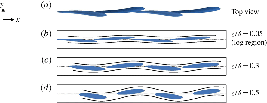
Conceptual three-dimensional interpretation of the shape and alignment of large low-momentum regions (blue iso-surface). (a) Illustration of the alternating one-sided streamwise vortices that flank these structures, and (b) the streamwise periodicity that occurs in the outer layer to the side of the large-scale structures. The shaded plane in (b) is approximately $0.2\unicode[STIX]{x1D6FF}$ to the side of the centreline of the structures.

Figure 8.

(a) Top view of the model. (b–d) Streamwise/spanwise wall-parallel slices.

Finally, we distil the above findings to create a conceptual representation of large-scale turbulence structure. The schematic drawing shown in figure 7 illustrates a ‘train’ of low-momentum regions. The appearance of each blue region adheres to the widely accepted representative/average shape, i.e. streamwise-elongated coherence with a shallow forward inclination angle. However, here we portray the structure to be slightly tilted from the vertical axis. As indicated here by figure 6 and by Kevin et al. (Reference Monty, Bai, Pathikonda, Nugroho, Barros, Christensen and Hutchins2017), this behaviour implies that non-symmetrical/one-sided streamwise vortex structures are dominant, and are formed underneath the leaning eruption of the low-momentum structure. Furthermore, if we take a streamwise/vertical slice at a spanwise location sideways from the spanwise centre of this train of structures, such as illustrated in figure 7(b), a repeating pattern will be evident in the outer layer. Figure 8(a) further displays the top view of this illustrative model. The importance here is that, when this train of structures is sliced horizontally in the log region, the velocity signature exhibits a weakly meandering behaviour. In the outer layer, however, this configuration will produce a wider signature with a stronger meandering tendency and a steeper tilting angle.

We note that these $\unicode[STIX]{x1D6FF}$ -scale behaviours closely resemble the buffer-layer model of Jeong et al. (Reference Jeong, Hussain, Schoppa and Kim1997), Schoppa & Hussain (Reference Schoppa and Hussain2002), and their temporal evolution can perhaps be inferred from the ‘minimal flow’ study shown in figure 24(c) in the review by Jiménez (Reference Jiménez2018). Overall, these similarities suggest that small- and large-scale coherence may exhibit similar unstable dynamical behaviour (Flores & Jiménez Reference Flores and Jiménez2010; Hwang & Cossu Reference Hwang and Cossu2010, Reference Hwang and Cossu2011), and that a self-sustaining mechanism not dissimilar to that proposed for the near-wall region exists at a hierarchy of scales across turbulent boundary layers.