2.1 Converging–diverging riblets

Here we use the same converging–diverging riblet surface as investigated by Kevin et al. (Reference Monty, Bai, Pathikonda, Nugroho, Barros, Christensen and Hutchins2017). A schematic of this surface is shown in figure 1(a,c), and readers are referred to Kevin et al. (Reference Monty, Bai, Pathikonda, Nugroho, Barros, Christensen and Hutchins2017) for the full physical surface specifications and its image. Unlike the vast majority of spanwise-varying roughnesses, the role of the C–D riblets is to give/induce a spanwise-varying ‘directionality’ to the flow, i.e. local direction of minimum resistance (Luchini, Manzo & Pozzi Reference Luchini, Manzo and Pozzi1991), which is along the yawed grooves. The yawed ribs themselves will most likely increase the overall surface drag for the height and spacing we use here. It should be noted however, that this study focuses on the large-scale three-dimensionality far above the surface, and does not attempt to resolve near-surface phenomena nor to seek a net drag reduction.

Figure 2.

(a,b) Mean streamwise velocity field of $xz_{2}$ and $xy_{1}$ plane PIV. Solid lines: local boundary layer thickness $\unicode[STIX]{x1D6FF}(x,y)$ . Dashed boxes: extent of field of view (FOV) captured by an individual camera. The FOV between cameras is overlapped for at least 12 mm in both streamwise and spanwise directions. Rib lines in (b) are not drawn to scale.

The rib height and spacing are $h^{+}=hU_{\unicode[STIX]{x1D70F}s}/\unicode[STIX]{x1D708}\approx 19$ and $s^{+}=sU_{\unicode[STIX]{x1D70F}s}/\unicode[STIX]{x1D708}\approx 26$ , yielding a blockage ratio of $h/\unicode[STIX]{x1D6FF}_{s}<0.009$ ( $U_{\unicode[STIX]{x1D70F}s}$ and $\unicode[STIX]{x1D6FF}_{s}$ are the friction velocity and boundary layer thickness of the smooth-wall base flow at matched Reynolds number). Figure 1(a) shows a schematic of the C–D pattern highlighting three spanwise locations of interest. The converging 

and diverging  sections are where low-speed (upwash) and high-speed (downwash) flows occur respectively, and lateral cross-flow is developed over the yawed ribs. Note that the C–D wavelength (i.e. spanwise periodicity) is $\unicode[STIX]{x1D6EC}=2.5\unicode[STIX]{x1D6FF}_{s}$ in the present experiments, while it was $1.5\unicode[STIX]{x1D6FF}_{s}$ in Kevin et al. (Reference Monty, Bai, Pathikonda, Nugroho, Barros, Christensen and Hutchins2017). This is due to the different base boundary layer thicknesses between the two studies. The degree of flow heterogeneity has been shown by Nezu & Nakagawa (Reference Nezu and Nakagawa1984), Vanderwel & Ganapathisubramani (Reference Vanderwel and Ganapathisubramani2015), Chung et al. (Reference Chung, Monty and Hutchins2018) to be dependent on the spanwise wavelength $\unicode[STIX]{x1D6EC}$ of the surface topography. In the present set-up we also observe different modified boundary layers compared to Kevin et al. (Reference Monty, Bai, Pathikonda, Nugroho, Barros, Christensen and Hutchins2017), due to slight variation in $\unicode[STIX]{x1D6EC}/\unicode[STIX]{x1D6FF}$ between studies. However, the bulk flow statistics are comparable, with the maximum strength of mean upwash velocity $W_{max}\approx 1.5\,\%U_{\infty }$ for both cases. Additionally, the flow behaviour that we emphasise here are large-scale turbulent features which are prevalent across all datasets.

2.2 Non-simultaneous PIV experiments

The measurements are conducted in an open-return boundary layer wind-tunnel facility in the Walter Basset Aerodynamics Laboratory at the University of Melbourne. This facility has been used in prior boundary layer studies (Perry & Marusic Reference Perry and Marusic1995; Harun et al. Reference Harun, Monty, Mathis and Marusic2013), and recently for a parametric study of the C–D riblets (Nugroho, Hutchins & Monty Reference Nugroho, Hutchins and Monty2013). Non-simultaneous large field-of-view PIV measurements are taken in three streamwise/vertical planes: over converging (upwash flow – called plane $xz_{1}$ ), diverging (downwash flow – plane $xz_{3}$ ) and yawed ribs (lateral cross-flow – plane $xz_{2}$ ); and in two streamwise–spanwise (wall-parallel) planes: in the logarithmic and outer regions (planes $xy_{1}$ and $xy_{2}$ respectively). Figure 1(b) displays a schematic of the present set-up. All experiments are conducted at a nominal free-stream velocity of $15~\text{m}~\text{s}^{-1}$ and at a streamwise development length of 4 m. All measurements are performed under zero-pressure-gradient conditions. The flows are seeded with polyamide particles with a mean diameter of $1~\unicode[STIX]{x03BC}\text{m}$ and illuminated using a dual cavity Big Sky Nd:YAG laser which delivers $120~\text{mJ}~\text{pulse}^{-1}$ . As indicated in figure 1(b), a 1 mm thick laser sheet is introduced from the wind-tunnel exit. Since the last optical component is far downstream from the measurement location (over 3 m distance, equating to approximately $60\unicode[STIX]{x1D6FF}$ ) with minimal blockage, no effects are observed in the turbulence statistics. The illuminated flows are imaged using PCO4000 cameras ( $4008\times 2672$ , 14-bit frame-straddled CCD, at $9~\unicode[STIX]{x03BC}\text{m}$ pixel size), equipped with Sigma 105 mm macro lenses. In the present configurations, the camera resolutions are 51 and $44~\unicode[STIX]{x03BC}\text{m}~\text{px}^{-1}$ for the vertical and wall-parallel measurements respectively. Figure 1(c) summarises the orthogonal PIV slices that will be considered in this paper. An acquisition rate of 1 Hz (per velocity realisation) is employed to ensure statistical independence, which is equivalent to approximately 260 boundary layer turnover times between consecutive snapshots. The time separation between particle-image pairs (or the laser pulse) itself is ${\sim}60~\unicode[STIX]{x03BC}\text{s}$ , or approximately 1.2 viscous time scales.

Figure 3.

Validation of velocity statistics for the smooth-wall base case at $Re_{\unicode[STIX]{x1D70F}}=2050$ . (a) Mean velocity, streamwise Reynolds stress and Reynolds shear stress. (b) Spanwise and wall-normal Reynolds stresses. Circles: $xz$ -plane PIV data (down sampled to 30 logarithmically spaced wall locations); squares: $xy$ -plane PIV data. Open symbols: statistics corrected using the method proposed by Lee, Kevin & Hutchins (Reference Lee, Monty and Hutchins2016); closed symbols: original attenuated Reynolds stresses. Solid lines show reference profiles from Sillero, Jiménez & Moser (Reference Sillero, Jiménez and Moser2013).

For the $xz$ -plane measurements, three cameras are used to capture a total of $0.52\times 0.11$ m streamwise/wall-normal domain, which corresponds to approximately $9.1\times 2.0$ $\unicode[STIX]{x1D6FF}_{s}$ . Here $\unicode[STIX]{x1D6FF}$ corresponds to the wall distance where the mean streamwise velocity reaches 99 % of the free-stream velocity. The resulting field of view for plane $xz_{2}$ is illustrated in figure 2(a). The obtained images are processed using an in-house PIV package previously used by Chauhan et al. (Reference Chauhan, Philip, de Silva, Hutchins and Marusic2014), Kevin et al. (Reference Monty, Bai, Pathikonda, Nugroho, Barros, Christensen and Hutchins2017), de Silva et al. (Reference de Silva, Baidya, Hutchins and Marusic2018) among others. A final interrogation window size of $24\times 24$ pixels with 50 % overlap is employed. This will result in a velocity vector spacing of approximately 0.55 mm (or 20 viscous units) in both in-plane directions. Together with the laser-sheet thickness, the spatial resolution in viscous units is $\unicode[STIX]{x0394}x^{+}\times \unicode[STIX]{x0394}y^{+}\times \unicode[STIX]{x0394}z^{+}\approx 41\times 36\times 41$ for the smooth-wall base case. For the wall-parallel $xy$ -plane measurements, five cameras are used to capture a total of $0.52\times 0.20~\text{m}$ of the streamwise/spanwise domain, which corresponds to approximately $9.1\times 3.5$ $\unicode[STIX]{x1D6FF}_{s}$ . The resulting FOV is represented in figure 2(b) for plane $xy_{1}$ . Note that the camera labelled C $_{1}$ is equipped with a Nikon 60 mm lens, hence yields a slightly reduced pixel resolution of $70~\unicode[STIX]{x03BC}\text{m}~\text{px}^{-1}$ . To compensate for this, C $_{1}$ is processed using an interrogation window size of $16\times 16$ pixels, which is smaller than that for C $_{2-5}$ . Together with the laser-sheet thickness, the spatial resolution in viscous units is $\unicode[STIX]{x0394}x^{+}\times \unicode[STIX]{x0394}y^{+}\times \unicode[STIX]{x0394}z^{+}\approx 54\times 54\times 36$ for the smooth-wall base case. Experimental and boundary layer parameters for all measurements are summarised in table 1. Three thousand instantaneous velocity realisations are taken for the riblets case and 2500 for the smooth-wall case. Flow statistics for the smooth-wall experiments are validated in figure 3, where the data points shown are down sampled to 30 wall-normal locations spaced logarithmically. The Reynolds stresses shown by the open symbols have been corrected using a method by Lee et al. (Reference Lee, Monty and Hutchins2016) to compensate for the spatial attenuation due to the volume averaging inherent in PIV interrogation, and the closed symbol shows the original attenuated PIV statistics. Overlaid are reference direct numerical simulation (DNS) statistics of Sillero et al. (Reference Sillero, Jiménez and Moser2013) at a comparable Reynolds number, where good collapse is observed between the statistics from the present measurements and the reference. The spatial statistics are also validated by comparing the two-point correlation function $R_{u^{\prime }u^{\prime }}$ with the profiles of Sillero, Jiménez & Moser (Reference Sillero, Jiménez and Moser2014) in figure 4. The results for both PIV orientations show good agreement with the DNS data.

Figure 4.

Validation of two-point correlation function of streamwise velocity of the smooth-wall base case measurements at $z_{ref}/\unicode[STIX]{x1D6FF}=0.1$ along the (a) streamwise and (b) spanwise directions. ○:  $xz$ -plane statistics; ▫:  $xy$ -plane statistics; solid lines: reference profiles from Sillero et al. (Reference Sillero, Jiménez and Moser2014). Not all PIV data points are shown for clarity.

Table 1.

Experimental parameters of the $xz$ and $xy$ PIV experiments.

a These quantities are local properties over the C–D surface.

b These quantities are spanwise averaged across one converging–diverging wavelength $\unicode[STIX]{x1D6EC}$ .

Figure 5.

Instantaneous total streamwise velocity over the C–D riblets. (a) In the cross-flow plane, reproduced from Kevin et al. (Reference Monty, Bai, Pathikonda, Nugroho, Barros, Christensen and Hutchins2017). Solid lines: wall heights of the corresponding horizontal planes. (b,c) In wall-parallel planes at $z/\unicode[STIX]{x1D6FF}_{s}=0.1$ and 0.5 respectively. A long contour of $u=0.6U_{\infty }$ (Gaussian filtered at $0.05\times 0.05\unicode[STIX]{x1D6FF}$ with $\unicode[STIX]{x1D70E}=2$ ) is drawn in (b). Note that these planes are acquired non-simultaneously.

4.1 Velocity coherence in the logarithmic region

Contour maps of streamwise correlation coefficients $R_{u^{\prime }u^{\prime }}$ in the $xz$ -planes are displayed in figure 8, where they are computed about a reference height of $z/\unicode[STIX]{x1D6FF}_{s}=0.1$ , or $z/\langle \unicode[STIX]{x1D6FF}\rangle _{\unicode[STIX]{x1D6EC}}=0.08$ , where $\langle \unicode[STIX]{x1D6FF}\rangle _{\unicode[STIX]{x1D6EC}}$ is the boundary layer thickness averaged across the C–D spanwise wavelength $\unicode[STIX]{x1D6EC}$ . Smooth-wall contours are also plotted at levels of 0.05 and 0.3 in grey shades to highlight the changes in lower and higher correlation values. Similar to observations in two-dimensional flows over smooth walls (Christensen Reference Christensen2001; Hutchins & Marusic Reference Hutchins and Marusic2007; Sillero et al. Reference Sillero, Jiménez and Moser2014, among others), all $R_{u^{\prime }u^{\prime }}$ maps of the modified flow feature inclined and streamwise-elongated coherent structures. In general, for the C–D riblet surface, both high and low correlation contours are physically shorter in the streamwise direction compared to the smooth-wall case, especially for lower $R_{u^{\prime }u^{\prime }}$ values (i.e. for larger coherence). The shortening of streamwise-velocity coherence is typical in flows with perturbed surfaces. Wu & Christensen (Reference Wu and Christensen2010) suggested several explanations for this, one of which is the reduction in streamwise spacing of consecutive vortices in the vortex packets. Flores, Jiménez & del Álamo (Reference Flores, Jiménez and del Álamo2007) on the other hand, suggested that lower mean shear over the perturbed surface leads to shorter low-momentum coherence. For larger roughness elements, Guala et al. (Reference Guala, Tomkins, Christensen and Adrian2012) concluded that the wake behind the object may have altered the natural streamwise coherence.

Figure 8.

Maps of $R_{u^{\prime }u^{\prime }}$ in streamwise/vertical planes about $z_{ref}/\unicode[STIX]{x1D6FF}_{s}=0.1$ , over (a–c) $xz_{1-3}$ respectively. Positive levels (solid lines) are 0.05, 0.15, 0.3; negative level (dashed line) is $-0.03$ . Grey shades: smooth-wall contour levels of 0.05, 0.3. Solid diagonal: inclination of the structure over $xz_{1-3}$ regions. Dot-dashed diagonal: inclination of the smooth-wall reference structure. Annotation NR indicates the negative region referred to in the text.

A comparison of the contour shapes in figure 8(a–c) also reveals different flow characteristics depending on spanwise location over the C–D surface. The inclination angle of the average structures for example (as illustrated by comparing each solid diagonal line with the smooth-wall dot-dashed reference), is steeper for the $xz_{3}$ plane compared to the $xz_{1}$ , due to its shorter aspect ratio. Note that here the inclination angle is computed from the linear fit through a locus of the maxima in $R_{u^{\prime }u^{\prime }}$ at each streamwise location, and only taken when the peak $R_{u^{\prime }u^{\prime }}$ value is larger than 0.05. Certainly, the streamwise extent of the large-scale coherence is much smaller for $xz_{3}$ (the diverging region shown in figure 8 c), than over the converging plane ( $xz_{1}$ , see figure 8 a). The most interesting feature however, occurs in the $xz_{2}$ plane over the yawed ribs. As shown by figure 8(b), the downstream ‘head’ of the inclined structure is curtailed when compared with the smooth-wall grey shaded contours, and a negatively correlated region (shown by the dashed contour and labelled ‘NR’) emerges in the outer layer. To give a better sense of the actual three-dimensional coherence; figure 9(a) displays the corresponding cross-stream correlation map $R_{u^{\prime }u^{\prime }}$ above the yawed region. The contours show a pronounced leaning average coherence, flanked by non-symmetrical anti-correlated regions. This picture suggests that the disappearance of the ‘head’ in the downstream $R_{u^{\prime }u^{\prime }}$ contour in figure 8(b) is because the upper part of this structure persistently exists at a different spanwise position (it has leant out of the $xz_{2}$ plane). Accordingly, we can also deduce that the taller negative contours on the positive $\unicode[STIX]{x0394}y$ side of the cross-stream map of figure 9(a), which are labelled ‘NR’, enter figure 8(b) at some downstream distance. This motion is also accompanied by statistically non-symmetrical vortical structures, as displayed by the $R_{u^{\prime }v^{\prime }}$ and $R_{u^{\prime }w^{\prime }}$ vectors shown in figure 9(b). Note that the $R_{u^{\prime }v^{\prime }}$ quantity can be interpreted as the event $v^{\prime }$ , for a given $u^{\prime }$ event. Hence, this stochastic estimation is analogous to a conditionally averaged $v^{\prime }$ structure, based on a particular $u^{\prime }$ event. The same description goes for $R_{u^{\prime }w^{\prime }}$ . The corresponding $R_{u^{\prime }u^{\prime }}$ map in the wall-parallel plane over the yawed region is displayed in figure 9(c). From this view, we notice that the positive contours are slightly yawed from the streamwise axis as indicated by the diagonal line. At first, the orientation may seem counter-intuitive since it opposes the direction of the yawed ribs. However, this averaged picture concurs with the cross-stream observation which is: the taller part of the structure (i.e. downstream) leans towards the downwash-flow region $xz_{3}$ .

Figure 9.

(a) Contours of $R_{u^{\prime }u^{\prime }}$ in the $yz$ plane, referenced at $z_{ref}/\unicode[STIX]{x1D6FF}_{s}=0.1$ over the yawed ribs. This correlation map is computed from the stereoscopic dataset of Kevin et al. (Reference Monty, Bai, Pathikonda, Nugroho, Barros, Christensen and Hutchins2017). Positive levels (solid lines) are 0.05, 0.15, 0.3; negative levels (dashed line) are $-0.05,-0.1$ . (b) Vectors of $R_{u^{\prime }v^{\prime }}$ and $R_{u^{\prime }w^{\prime }}$ . (c) Contours of $R_{u^{\prime }u^{\prime }}$ in $xy_{1}$ plane. Annotation ‘NR’ indicates the negative region referred to in the text.

This overall kinematics can be better described using the schematic drawn in figure 10. Here the large turbulence structure is portrayed to be slightly inclined/angled from both the $x$ and $z$ axes, as suggested by the $R_{u^{\prime }u^{\prime }}$ correlation results in the $xy$ and $yz$ planes (shown in figures 9(a) and 9(c) respectively). The series of lateral arrow annotations indicate the spanwise sign of the mean roll modes $\pm V$ near to and away from the surface. Notice that, due to the its forward inclination/ramping (Adrian et al. Reference Adrian, Meinhart and Tomkins2000; del Álamo et al. Reference del Álamo, Jiménez, Zandonade and Moser2006), the lateral velocities $\pm V$ are not equally distributed across the structure. The taller downstream head will mostly experience $-V$ , while the lower upstream tail will experience a $+V$ from the time-averaged secondary flow. This is further illustrated by the symbols over the $R_{u^{\prime }u^{\prime }}=0.05$ contour in the $xz_{2}$ plane inset. This uneven distribution ( $-V$ at the downstream end and $+V$ at the upstream) thus manifests as a net torque as indicated by the rotational sign above the structure, as well as the leaning behaviour observed by Kevin et al. (Reference Monty, Bai, Pathikonda, Nugroho, Barros, Christensen and Hutchins2017) in the cross-stream plane.

Figure 10.

Schematic of an inclined low-speed structure over the yawed part of the C–D surface. Series of arrow annotations indicate the mean lateral velocities or the secondary flows, near ( $+V$ ) and away ( $-V$ ) from the surface. The $xz_{2}$ plane projects the $R_{u^{\prime }u^{\prime }}=0.05$ previously shown in figure 8(b), with symbols also indicating the direction of lateral mean velocity $V$ . Rotational sign: the rotational direction (about the vertical axis) experienced by this structure.

To deduce the possible dynamics of this large-scale behaviour, we firstly need to realise that the rib dimensions are small ( $h/\unicode[STIX]{x1D6FF}<1\,\%$ ), and their direct effects on the flow are restricted only to regions immediately above the surface. This is by means of imposing directional resistance to the flow (Luchini et al. Reference Luchini, Manzo and Pozzi1991). However, on the line of convergence of the rib pattern, the spanwise flows over the yawed riblets meet each other and are redirected upwards, creating the large-scale ejections depicted in figure 5(a). These vertical ejections and the resultant large-scale secondary flows lead to lateral momentum transfer away from the converging section (far from the surface), as depicted by the $-V$ arrows in figure 10. This large-scale motion overrides any near-wall effects due to the yawed riblets, and causes the structure in figure 10 to yaw to the right, opposing the rib direction underneath it. Therefore, one can consider that the misalignment direction of the large structures in the present case is not strictly a direct effect of the yawed ribbed surface, but is due to the presence of the overall secondary flows. In other words, we would expect to see similar yawed behaviour of large-scale structures in any flow with embedded large-scale streamwise vortices. Indeed, the streamwise-misaligned behaviour in the $R_{u^{\prime }u^{\prime }}$ correlation map, as well as the asymmetry in the flanking anti-correlated regions, are also observable in other three-dimensional boundary layer datasets over various surfaces. A few of examples are in the boundary layer developed over the spanwise-heterogeneous roughness (Bai et al. Reference Bai, Kevin, Hutchins and Monty2018), and over a smooth-wall boundary layer developed downstream of vortex-generator devices (Baidya et al. Reference Baidya, de Silva, Huang, Castillo, Marusic and Hutchins2016). The large multi-plane FOVs captured in the present measurements have offered a more detailed illustration of this prevalent behaviour, and further observation in the outer layer will be presented in the § 4.2.

Figure 11.

(a–c) Maps of $R_{u^{\prime }u^{\prime }}$ in streamwise/vertical planes with $z_{ref}/\unicode[STIX]{x1D6FF}_{s}=0.5$ , for the $xz_{1-3}$ planes respectively. Positive levels (solid lines) are 0.05, 0.15, 0.3; negative levels (dashed lines) are $-0.025,-0.05$ . Grey shaded contours: smooth-wall contour levels of 0.05, 0.3.

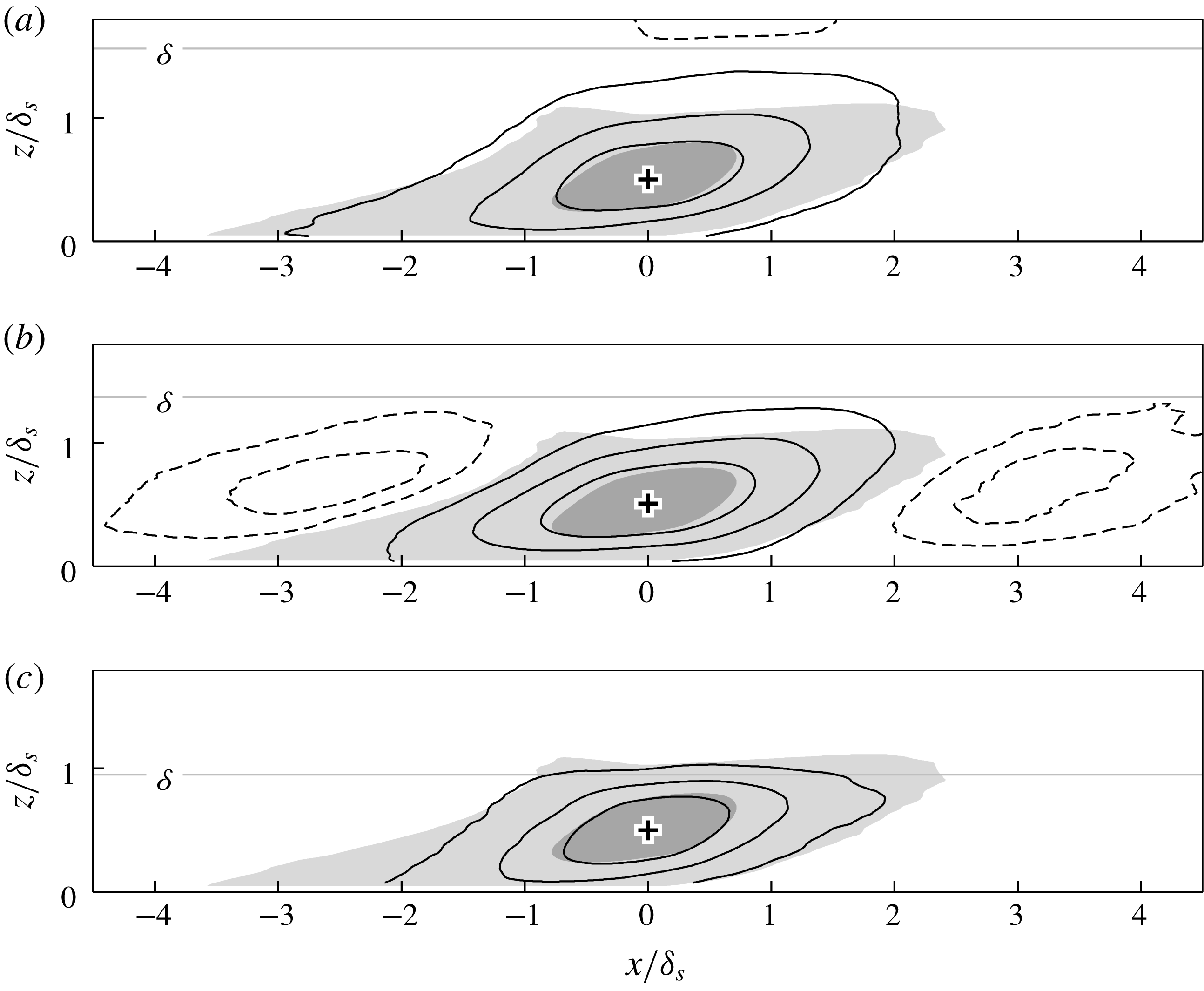
4.2 Velocity coherence in the outer layer

Since the outer-layer structures exhibit a lateral unstable tendency (as evidenced anecdotally in figure 5 c), it will be interesting to see how this behaviour manifests statistically. Additionally, it is well known that outer-layer structures between smooth and rough surfaces show excellent qualitative agreement (Volino, Schultz & Flack Reference Volino, Schultz and Flack2007, Reference Volino, Schultz and Flack2011; Squire et al. Reference Squire, Morril-Winter, Hutchins, Marusic, Schultz and Klewicki2016), which concurs with Townsend’s Reynolds number similarity hypothesis (Townsend Reference Townsend1976). The exception in this regards are the continuous spanwise-aligned rods of Krogstadt & Antonia (Reference Krogstadt and Antonia1999) and the spanwise-aligned bars of Volino, Schultz & Flack (Reference Volino, Schultz and Flack2009). In those cases of continuous spanwise elements, the near-wall flow is forced upwards over the roughness elements leading to strong local ejections. This leads to roughness effects that penetrate further into the outer layer. To a certain degree, the mechanism we observe here is analogous to the above situation, i.e. we have continuous yawed grooves. However, here the resulting ejections occur along lines in the streamwise direction (i.e. over the converging region), instead of uniformly occurring along the spanwise direction, as is for the case for spanwise bars/rods. For the converging–diverging riblets, these ejections aligned along the converging regions set up large-scale secondary flows, and as a result, the roughness sublayer (the part of the flow that feels the effects of the roughness topography) essentially extends to the edge of the layer, and no outer-layer similarity can occur.

Figure 11 displays $R_{u^{\prime }u^{\prime }}$ maps for the $xz_{1-3}$ planes with $z_{ref}/\unicode[STIX]{x1D6FF}_{s}=0.5$ (equivalent to 60 roughness heights away from the surface), clearly showing signs of this three-dimensionality. In general, contours of $R_{u^{\prime }u^{\prime }}>0.3$ seem comparable between plots, but larger coherence is distinctively different. This in part can be explained by the spanwise variation in the local boundary layer thickness between the three planes. For instance, the flat upper contours in the $xz_{3}$ map are due to the proximity to the free-stream flow, reflected in the reduced local boundary layer thickness over the diverging region. The most intriguing observation, however, is the large streamwise-repeating pattern in the $xz_{2}$ plane of figure 11(b), which has a streamwise distance (between minima) of approximately $5.6\unicode[STIX]{x1D6FF}_{s}$ or $4.6\langle \unicode[STIX]{x1D6FF}\rangle _{\unicode[STIX]{x1D6EC}}$ . This pattern does not appear in the smooth-wall correlation, or in the $xz_{1}$ and $xz_{3}$ planes (which are only $0.65\unicode[STIX]{x1D6FF}_{s}$ away in the spanwise direction). As discussed in § 3, we surmise that these regions of detached coherence arise from the leaning ejections over the converging riblets. Figure 11(b) shows that this behaviour exhibits some degree of streamwise periodicity. Figure 12 shows the corresponding wall-parallel slice of the correlation map over the yawed riblets at $z_{ref}/\unicode[STIX]{x1D6FF}_{s}=0.5$ . Here, the streamwise-repeating pattern is also clearly apparent, with the stronger anti-correlated region flanking in the positive $y$ direction (as previously suggested by the correlation map in figure 9(a) at the wall-normal location of $z/\unicode[STIX]{x1D6FF}_{s}=0.5$ ). All of these observations are consistent with a low-momentum region meandering about the converging region, with an apparent streamwise wavelength of approximately $5.6\unicode[STIX]{x1D6FF}_{s}$ . As a side note, when we take a reference correlation point $y_{ref}$ closer to the $xz_{1}$ /converging region, the repeating pattern becomes less apparent (and eventually disappears altogether when $y_{ref}/\unicode[STIX]{x1D6EC}=0.5$ ). This is due to the cancellation from the opposite-signed pattern, coming from the opposing yawed region (i.e.  $y/\unicode[STIX]{x1D6EC}=0.75$ ). Hence, the average structure will appear more similar to the more well-known smooth-wall coherence.

Figure 12.

Maps of $R_{u^{\prime }u^{\prime }}$ in $xy_{2}$ plane ( $z_{ref}/\unicode[STIX]{x1D6FF}_{s}=0.5$ ), over the yawed riblets. Positive levels (solid lines) are 0.025, 0.05, 0.15, 0.3; negative level (dashed line) are $-0.025,-0.05,-0.1$ . Shaded region illustrates the association of the alternating pattern with the highly meandering structure.

To some degree, this outer-layer alternating behaviour is similar to that observed by Elsinga et al. (Reference Elsinga, Adrian, Oudheusden and Van Scarano2010), where the pattern became more apparent in their filtered velocity fields. They suggested that larger vortex organisation is responsible for this behaviour, and provide a conceptual sketch of this (figure 16 in their publication). In their proposed interpretation, outer-layer structures ride over two adjacent log region structures in an alternating manner, giving rise to a diagonal-like pattern in the (filtered) swirling–strength correlation. For the present case however, this outer-layer pattern arises from the fact that tall low-momentum regions turn laterally in the outer layer, manifesting as an aggressive meandering of low-momentum large-scale streaks in the wake region. In other words, the elongated log region streak over the converging region will meander, causing the alternating pattern to appear in correlations computed just to the side of this region (here over the yawed ribs). Additionally, we have shown from stochastic estimation that this streamwise-misaligned behaviour is accompanied by non-symmetrical streamwise vortex structures (figure 9(b) – see also Kevin et al. (Reference Monty, Bai, Pathikonda, Nugroho, Barros, Christensen and Hutchins2017)), while for the case of Elsinga et al. (Reference Elsinga, Adrian, Oudheusden and Van Scarano2010) symmetrical hairpin-type vortices were inferred.

Figure 13.

(a) Grey shaded areas: contours of filtered velocity $u<0.85U_{\infty }$ . Thin line: mean spanwise location, or the spine, of the grey region for each $x$ grid (here plotted only for the largest grey area). Thick line: the smoothened spine contour, showing the minimum $y$ location in the contour taken as a reference averaging point. (b) Conditional average of turbulent fluctuation about the reference point shown in (a). Solid/dashed contour shows $\overline{u^{\prime }}_{cond}=\pm 0.1U_{\unicode[STIX]{x1D70F}s}$ . (c) The conditional vector fields $\overline{u^{\prime }}_{cond},\overline{v^{\prime }}_{cond}$ . Vector spacing are down sampled by 10 for clarity.

To further relate the above observation to the aggressive meandering of the low-speed event in the outer layer, we perform a brief conditional-averaging analysis on the retarded flow structure. The grey shaded areas in figure 13(a) show the streamwise velocity regions $u_{f}<85\,\%U_{\infty }$ , after the flow field is low-pass filtered. To do that, the original velocity matrix is convolved with a smaller matrix of Gaussian distribution (with a kernel size equivalent to $0.25\times 0.25\unicode[STIX]{x1D6FF}_{s}$ and $\unicode[STIX]{x1D70E}=2$ ). Hence, turbulence fluctuation smaller than this filter size will be removed. The ‘spine’ of each binary structure is then found by taking the mean spanwise location of each connected region at every $x$ grid. The location of this spine is shown by the thin fluctuating line along the structure. We then further smooth this spine location using a $1\unicode[STIX]{x1D6FF}_{s}$ one-dimensional Gaussian kernel of 1 $\unicode[STIX]{x1D6FF}_{s}$ and $\unicode[STIX]{x1D70E}=2$ (shown by the thick black line in figure 13 a), and use the smoothed location to obtain the minimum spanwise position of this large-scale meandering behaviour. Note that we only consider the longer spines which extend for more than $3\unicode[STIX]{x1D6FF}_{s}$ in the streamwise direction. Accordingly, conditionally averaged events are conditioned on the spanwise minima of this meandering spine. This condition location is illustrated in figure 13(a) by the $+$ symbol and the annotation ‘reference point’. The conditionally averaged flow field with respect to this minimum $y$ position is shown in figure 13(b), where the solid and dashed contours indicate the conditional mean $\overline{u^{\prime }}_{cond}=\pm 0.1U_{\unicode[STIX]{x1D70F}s}$ respectively. This result complements the correlation map shown figure 12, further highlighting a dominant meandering behaviour with an average wavelength of approximately $6\unicode[STIX]{x1D6FF}_{s}$ . The corresponding averaged vector field $\overline{u^{\prime }}_{cond},\overline{v^{\prime }}_{cond}$ is shown in figure 13(c), clearly showing the one-sided wall-normal vortex structure associated with this outer-layer meandering. Note that changing the filter size and the velocity threshold used throughout this process (even by $\pm 50\,\%$ ) has a negligible effect on this dominant instantaneous large-scale behaviour.

The merit of analysing large low-momentum streaks in spanwise-heterogeneous flow is that their position is fixed in space, compared to the random distribution occurring in the spanwise-homogeneous boundary layers. At present, our closest description of these kinematics is provided by the low-speed streak model in the buffer layer as suggested by Jeong et al. (Reference Jeong, Hussain, Schoppa and Kim1997) (figure 10 in their publication), only in this instance we observe similar features in the logarithmic and outer layer, and at much larger scale. In that model, the wavy low-speed streak is flanked by streamwise-alternating positive and negative asymmetrical vortex tubes (further shown by Schlatter et al. Reference Schlatter, Li, Örlü, Hussain and Henningson2014, to be inclined and tilted). Note that the overlapping upper/lower streamwise vortices (with opposite sign) drawn in Jeong et al. (Reference Jeong, Hussain, Schoppa and Kim1997) also statistically appear within the present flow, as shown in figure 13 of Kevin et al. (Reference Monty, Bai, Pathikonda, Nugroho, Barros, Christensen and Hutchins2017) and here in figure 9(b). Our observations give further evidence that small- and large-scale coherence exhibit very similar unstable dynamical behaviour, as mentioned by Flores & Jiménez (Reference Flores and Jiménez2010), Hwang & Cossu (Reference Hwang and Cossu2010, Reference Hwang and Cossu2011).

As a final important point, in a separate study (yet to be published) we recently conducted very large field-of-view PIV over a smooth wall with embedded large-scale streamwise vortices produced by vortex generator devices, similar to Baidya et al. (Reference Baidya, de Silva, Huang, Castillo, Marusic and Hutchins2016). In this case a very similar alternating behaviour is also strongly present. This indicates that the turbulent behaviours we describe here are prevalent in vortex-embedded wall flows (in spanwise-heterogeneous roughness for instance), and not specific to the case of herringbone-type riblets.