CPSS system-of-systems level design

The design of CPSS architecture at the system-of-systems level needs to incorporate several factors. First, given the evolution nature of cyber and physical technologies, adaptability that enables the capabilities of self-learning, self-organization, and context awareness is important to design open systems that can evolve along technology advancement (Horváth and Gerritsen, Reference Horváth and Gerritsen2012; Tavčar and Horváth, Reference Tavčar and Horváth2018). Using new technologies as the augmentation to existing products can effectively enhance adaptability (Vroom and Horváth, Reference Vroom and Horváth2014). Second, the complexity of the CPSS has significantly increased from traditional products and devices. The CPSS products are connected through Internet of Things and heavily rely on data exchange from each other to realize their functions. Communication between devices plays a major role. Therefore, how to design systems of CPSS which have dependable communication is important. Reliable large-scale networked systems that do not fail are impossible to achieve. Resilient systems that can recover automatically from partial failures are more likely to be realized (Wang, Reference Wang2016, Reference Wang2018a). Third, the high-dimensional design space of CPSS includes not only the cyber and physical subspaces but also the social subspace. Examples of the emerging research issues are how to design the modalities for human–system interaction (Horváth and Wang, Reference Horváth and Wang2015), how to enable context awareness and personalized communication between CPSS and humans (Li et al., Reference Li, Horváth and Rusák2018), and how to quantify trustworthy strategic relationships for information sharing (Wang, Reference Wang2018b, Reference Wang2018c, Reference Wang2018d, Reference Wang and Fukuda2020b, Reference Wang2021b).

Network connectivity is essential for CPSS. A standalone CPSS device cannot perform the functions which it is designed for. Compared to traditional products, the design of CPSS devices requires engineers to have a better understanding of the system level behaviors, as well as the new methodology for the optimization at the network scale. Systems level modeling methods and tools have been developed for CPSS design and analysis, such as hybrid discrete-event and continuous simulations (Jeon et al., Reference Jeon, Chun and Kim2012; Lee et al., Reference Lee, Hong and Kim2015a, Reference Lee, Niknami, Nouidui and Wetter2015b), inductive constraint logic programming (Saeedloei and Gupta, Reference Saeedloei and Gupta2011) abductive reasoning (Horváth, Reference Horváth2019), hybrid timed automaton (Burmester et al., Reference Burmester, Magkos and Chrissikopoulos2012), ontologies (Petnga and Austin, Reference Petnga and Austin2016), information schema (Pourtalebi and Horváth, Reference Pourtalebi and Horváth2017), UML (Magureanu et al., Reference Magureanu, Gavrilescu, Pescaru and Doboli2010), and SysML (Palachi et al., Reference Palachi, Cohen and Takashi2013).

Information diffusion in CPSS networks

The information flow in computer networks and social networks has been studied by researchers. The propagation of information can be modeled in different ways. The most used approach is the epidemic model of networks, where transmission probabilities of virus between nodes are mainly used to model the speed of infection and the dynamics of outbreak and decay is captured with ordinary differential equations (Newman, Reference Newman2002; Wu et al., Reference Wu, Huberman, Adamic and Tyler2004). The epidemic model has been widely applied to study the propagation of keywords or phrases among blogs (Gruhl et al., Reference Gruhl, Guha, Liben-Nowell and Tomkins2004) and within social networks (Kleineberg and Boguná, Reference Kleineberg and Boguná2014). In the linear influence model (Yang and Leskovec, Reference Yang and Leskovec2010), the propagation of information is modeled and parameterized by the influences of individual nodes in the network. In the event-driven modeling approaches, the adoption of new information by nodes is characterized by discrete Poisson processes (Simma and Jordan, Reference Simma and Jordan2010; Iwata et al., Reference Iwata, Shah and Ghahramani2013) or continuous hazard function (Du et al., Reference Du, Song, Woo and Zha2013).

Very limited work has been done in studying information diffusion in CPSS networks. Yagan et al. (Reference Yagan, Qian, Zhang and Cochran2013) studied the information transmission in the coupled social and physical networks according to the epidemic model. Lu et al. (Reference Lu, Lv, Jiao, Wang and Liu2015) investigated how to maximize the information diffusion in CPSS networks when nodes are connected probabilistically. Wang et al. (Reference Wang, Jiang, Han, Quek and Ren2017) used a game theoretic approach in combination with the epidemic model at the system level to study the effects when nodes make local decisions of forwarding information to others. Yi et al. (Reference Yi, Zhang and Gan2019) defined the states of each node in both physical and social spaces for the epidemic model so that the mutual influence between social behavior spread and multimedia data transmission can be revealed. Wang (Reference Wang2020a, Reference Wang2021a) developed statistical approaches where copula and VAR models were used to model the information correlations among CPSS nodes.

Given that CPSS nodes possess local functions of sensing, computing, and decision making, we need to study not only how information propagates but more importantly how the information propagation directly affects these functions. In the proposed models, the propagation of information elements is not modeled directly. Rather, the dynamic effect of information diffusion, which is the change of the sensing and computing capabilities of CPSS nodes, is used to quantify the information dynamics. That is, the dynamic changes of those capabilities along time are directly captured in the proposed information dynamics models. The sensing and computing capabilities of CPSS are quantified based on a probabilistic graph model, as introduced in the next section.

Probabilistic graph model

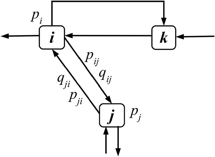
A recently developed probabilistic graph model (Wang, Reference Wang2018a) for CPSS networks is the foundation of the proposed information dynamics models. In the probabilistic graph model, each node has its own sensing, reasoning, and communication units. As illustrated in Figure 1, there are probabilities associated with information gathering and exchange between nodes. For each node, there is a prediction probability indicating the capabilities of information gathering and reasoning. For each directed edge indicating information exchange, there are reliance probabilities associated with it. The two types of probabilities are defined as follows.

Fig. 1.

Probabilistic graph model of CPSS systems.

The prediction probability that the k-th node detects the true state of world θ is

(1)$${{\mathbb P}}( {x_k = \theta } ) = p_k,$$

where x _k is the state variable. For convenience, we denote q _k = 1 − p _k. The information dependency between nodes i and j is modeled with P-reliance probability

(2)$${{\mathbb P}}( {x_j = \theta {\rm \vert }x_i = \theta } ) = p_{ij},$$

which is the probability that the j-th node predicts the true state of the world given that the i-th node predicts correctly. Similarly, we also have Q-reliance probability

(3)$${{\mathbb P}}( {x_j = \theta {\rm \vert }x_i\ne \theta } ) = q_{ij},$$

because nodes could be negatively correlated, or miscommunication between nodes could exist. The reliance probability can be used to model reliability of communication between nodes, for example, in moving vehicles’ ad hoc wireless networks, data packet loss is not uncommon.

Therefore, different from the adjacency matrix in traditional graph model with binary “yes-or-no” edge connection topology, there are reliance probabilities associated with each pair of nodes in the new probabilistic graph model. If the communication channel from node i and node j is disrupted, both p _ij and q _ij are zeros.

The random state variables with binary values (=θ or  ≠ θ) can be extended to multiple values or continuous. For instance, one sensor measures a value (e.g. temperature or flow speed) which follows some distribution, as in prediction probability. If there are a finite set of possible values {θ ₁, …, θ _N} for state variables. The prediction probability ℙ(x _k = θ _n) and reliance probability ℙ(x _j = θ _n|x _i = θ _m), where 1 ≤ m, n ≤ N, can be enumerated similarly. As a simplification without loss of generality, in this paper, we assume that the state variables take binary values.

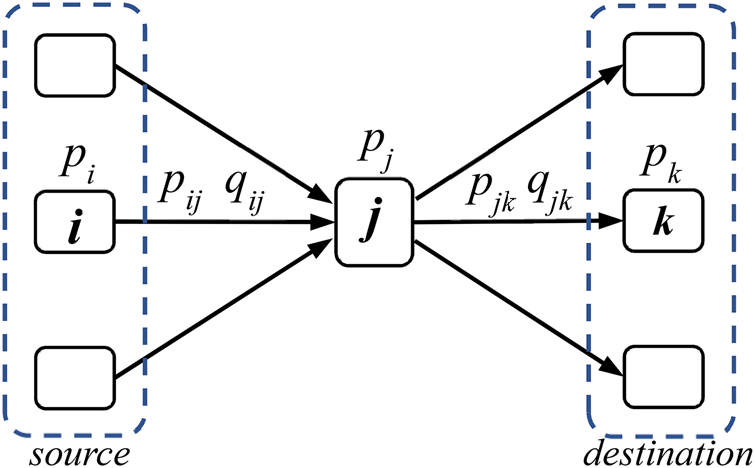
The edges in the probabilistic graph are directional. The neighbors of each node can be further differentiated as source nodes or destination nodes, as illustrated in Figure 2. For one node, its source nodes are those sending information to this node, whereas the destination nodes are those receiving information from it. When receiving different cues from source nodes, a CPSS node can update its prediction probability to reflect its perception of the world. The aggregation of prediction probabilities sensitively depends on the rules of information fusion during the prediction update.

Fig. 2.

Source and destination nodes with respect to node j.

If P(x _k) and $P( {x_k^C } )$ denote the probabilities of a positive and a negative prediction from node k, respectively, we define the best-case fusion rule as

(4)$$\eqalign{& {P}^{\prime}( {x_k} ) = \cr & 1-( {1-P( {x_k} ) } ) \mathop \prod \limits_{i = 1}^{M_P} P( {x_i} ) ( {1-P( x_k\vert x_i) } ) \!\mathop \prod \limits_{\,j = 1}^{M_N} P( {x_j^C } ) ( {1-P( x_k\vert x_j^C )} )},$$

where node k updates its prediction based on its own current prediction and those cues from its M _P + M _N source nodes, out of which M _P of the source nodes provide positive predictions whereas M _N of them provide negative predictions, P(x _k|x _i) indicates the probability that a positive message from node i leads to a positive prediction of node k, and $P( x_k\vert x_j^C )$ is the probability that a negative message from node j leads to a positive prediction of node k. Therefore, if any of the cues from the source nodes are positive, the prediction of the node is positive. Some variations of this fusion rules exist. For instance, the previous prediction from itself can be either included or excluded during the update.

Similarly, the worst-case fusion rule can be defined as

(5)$${P}^{\prime}( {x_k} ) = P( {x_k} ) \mathop \prod \limits_{i = 1}^{M_P} P( {x_i} ) P( x_k\vert x_i) \mathop \prod \limits_{\,j = 1}^{M_N} P( {x_j^C } ) P( x_k\vert x_j^C ). $$

That is, if any of the cues from the source nodes is negative, the prediction of the node is negative. The Bayesian fusion rule is defined as

(6)$${P}^{\prime}( {x_k} ) = \displaystyle{{P( {x_k} ) \mathop {\max }\limits_{\rm P} { {{( {P( {x_k} ) } ) }^r{( {1-P( {x_k} ) } ) }^{S-r}} } } \over {\smallint {( {P( {x_k} ) } ) }^r{( {1-P( {x_k} ) } ) }^{S-r}{\rm d}P}},$$

where the prediction of the node is updated to P ^′ from prior prediction P, and out of S cues that the neighboring nodes provide, r of them provide are positive, if the maximum likelihood principle is taken.

The probabilistic graph model provides a system level abstraction and a mesoscale description of CPSS networks, where information exchange and aggregation are captured with the overall probabilistic measures instead of the detailed level of information elements. More details about the probabilistic graph model can be found in Wang (Reference Wang2018a).

Vector autoregression models

VAR models provide a direct approach to represent time-dependency and mutual influences between variables in time series problems. In traditional VAR models, it is assumed that all variables are linearly dependent on each other for each intermediate step. Here, a latent variable VAR and a topology-informed VAR model are proposed. The prior knowledge of network topology is incorporated in model training, and functional dependency between nodes is directly modeled with the adjacency information. That is, two prediction probabilities are functionally related to each other at two immediate time steps only if there is a direct connection between the two nodes. This approach can reduce the number of parameters to be trained and improve the training efficiency.

Topology-informed VAR

The traditional VAR time series model is

(9)$${\boldsymbol P}( s ) = {\boldsymbol A}_0 + \mathop \sum \limits_{l = 1}^L {\bf A}_l{\boldsymbol P}( {s-l} ) + {\rm \epsilon },$$

where the values of prediction probabilities for all n nodes at the s-th time step form the column vector P(s) = (P ₁(s), …, P _n(s)). The prediction probabilities at the s-th time step are dependent on the values of P(s − 1), …P(s − L) at all the previous L steps. A₀ ∈ ℝⁿ is the column vector of intercepts that indicate the bias. The noise ${\rm \epsilon }\sim {\cal N}( {0, \;{\bf \Sigma }_\epsilon } )$ is modeled as the multi-variant normal random variable, and the n × n coefficient matrices ${\bf A}_l$'s capture the interdependency between prediction probabilities. The VAR model in Eq. (9) captures the time and location dependencies of nodes simultaneously as the linear relationships. The time series model captures the memory effect where the data sharing history in the previous L steps affects the current values. It also implicitly captures the potential effect of possible delays in communication, where data arriving at a node could be sent by other nodes several time steps before. The positive or negative signs of the elements in ${\bf A}_l$'s indicate the positive or negative correlations of the pairs. The correlations will cause fluctuations of the P values between 0 and 1.

One issue of VAR for network modeling is that the number of parameters increases quadratically as the number of nodes increases. In the topology-informed VAR model, not all parameters in Eq. (9) are equally important. If one node is connected with and shares information directly to another node, the information dependency is more evident than those that are not directly connected. Therefore, the topology of the network provides indications of dependency. This prior knowledge can be applied to the VAR model as the constraints to reduce the effective coefficients and simplify the model training process. In a sparsely connected network, dependency between nodes is loose, and the number of effective coefficients becomes small. This will improve the efficiency of the training process where the required training data size can be reduced accordingly.

The topology-informed VAR model is defined as

(10)$${\boldsymbol P}( s ) = {\boldsymbol A}_0 + \mathop \sum \limits_{l = 1}^L ( {{\bf D}^T\circ {\bf A}_l} ) {\boldsymbol P}( {s-l} ) + {\rm \epsilon },$$

where ${\bf D} = ( {d_{ij}} ) _{n \times n}$ is the adjacency matrix of the network with n nodes. Its elements are d _ij = 1 if a directed edge exists from node i to node j, and d _ij = 0 otherwise. The diagonal elements d _ii = 1 for all i's. In addition, T is the matrix transpose operator, and ∘ is the element-wise product or Hadamard product between two matrices.

In the original VAR model in Eq. (9), the number of parameters or coefficients that need to be calibrated through training is n + n ²L. When the topology is considered as the constraint, the number of parameters is reduced to n + eL where e is the number of directed edges in the graph. The reduction is significant if the nodes are sparsely connected. With a smaller number of parameters, the training or data fitting process can be more efficient where the required number of training data points for good fitting is also reduced. Note that the topology-informed VAR is reduced to the original VAR when the network is fully connected.

The training of topology-informed VAR model in Eq. (10) can be implemented as a constrained optimization problem, where the loss or error of model prediction is minimized subject to constraint

(11)$$\mathop \sum \limits_{l = 1}^L \Vert {( \bf \Pi-{\bf D}^T) } \circ {{\bf A}_l} \Vert = 0,$$

where Π is a matrix with the same size of ${\bf D}$ and all elements are 1's. ∥ ⋅ ∥ is the matrix norm which quantifies the distance to the origin and can be calculated with L ₂ norm.

Constrained nonlinear optimization algorithms can be applied to solve this training problem. Because the elements in coefficient matrices ${\bf A}_l$'s contain the physical meanings of adjacency between nodes, they are also related to the reliance probabilities as described in Section “Probabilistic graph model”. Therefore, the coefficients can also be treated as probabilities. The values of the coefficients can be further constrained to between 0 and 1.

Notice that all coefficients and parameters of the VAR models can be time-dependent. When the network topology dynamically changes, the model parameters need to be re-calibrated to reflect the changes. One advantage of data-driven modeling is that the model parameters can be updated frequently once new datasets are available. The proposed VAR models can be readily applied to the dynamic CPSS networks where the topology is not fixed and evolves along time.

Latent variable VAR

More complex models can be applied to capture the functional interdependency between prediction probabilities. Here, latent variables or hidden state variables are introduced to capture the inherent correlations between prediction capabilities. The latent variable VAR model is defined as

(12)$${\boldsymbol P}( s ) = {\bf B}{\boldsymbol Y}( s ) + {\boldsymbol \eta },$$

(13)$${\boldsymbol Y}( s ) = \mathop \sum \limits_{l = 1}^L {\bf T}_l{\boldsymbol Y}( {s-l} ) + {\boldsymbol \varepsilon },$$

where Eq. (12) captures the relation between observable P ∈ ℝⁿ and hidden state or latent variables Y ∈ ℝ^K, and the evolution of hidden state variables as state transition is modeled in Eq. (13). Here, ${\bf T}_l\in {{\mathbb R}}^{K \times K}$ (l = 1, …, L) is the coefficient matrix that captures the dependency between the hidden state variables, and ${\bf B}\in {{\mathbb R}}^{n \times K}$ is the observation matrix. Notice that the dimension of state vector Y is not necessarily the same as the dimension of observable vector P. The number of hidden state variables is typically less than that of the observable in a correlated system, that is K ≤ n. ${\boldsymbol \eta }\sim {\cal N}( {0, \;{\bf \Sigma }_\eta } )$ and ${\boldsymbol \varepsilon }\sim {\cal N}( {0, \;{\bf \Sigma }_\varepsilon } )$ are associated with the noises of observation and state transition, respectively, and modeled as multi-variate normal variables. In the hidden state model, the interdependency among nodes is captured through the hidden state variables. The direct correlations between state variables cause the inherent correlations between the observables so that more complex dependency relations are captured.

In the VAR model in Eq. (9), the parameters to be calibrated are vector A₀, matrices ${\bf A}_l$'s, and covariance matrix ${\bf \Sigma }_\epsilon$. For the latent variable VAR model in Eqs (12) and (13), the parameters to be calibrated or trained include ${\bf T}_l$'s, ${\bf B}$, as well as ${\bf \Sigma }_\eta$ and ${\bf \Sigma }_\varepsilon$. The Expectation-Maximization (EM) algorithm (Bańbura and Modugno, Reference Bańbura and Modugno2014) can be applied to train the model with a large number of parameters. The EM algorithm consists iterations of two alternating steps. In the E-step, the expectation of the log-likelihood for hidden state variables and the available training dataset conditional on the parameters $\Lambda = { {{\bf T}_l, \;{\bf B}, \;{\bf \Sigma }_\eta , \;{\bf \Sigma }_\varepsilon } }$ is calculated. The available training dataset ${\cal P}$ is the time series of prediction probabilities P's. The hidden state variables ${\cal V}$ include all Y's. The expectation of the log-likelihood at the k-th iteration is calculated as ${{\mathbb E}}( {\log f( {{\cal P}, \;{\cal V}{\rm \vert }{\Lambda }^{\prime}} ) \vert \Lambda^{( {k-1} ) }} )$. In the M-step, the parameters are updated by solving the maximization problem $\Lambda ^{( k ) } = {\rm argma}{\rm x}_{{\Lambda }^{\prime}}{{\mathbb E}}( {\log f( {{\cal P}, \;{\cal V}{\rm \vert }{\Lambda }^{\prime}} ) \vert \Lambda^{( {k-1} ) }} )$. The E-step and M-step are applied iteratively until the parameters converge.

When the number of latent variables K is the same as the number of the observable n, the latent variables can be interpreted as the state variables associated with the individual nodes. The coefficients ${\bf T}_l$'s then can be regarded as the associations between nodes in information exchange, similar to the topology-informed VAR model in Section “Topology-Informed VAR”. Similarly, the network topology can be applied as constraints to simplify the model training process. In the topology-informed latent variable VAR model, the state transition in Eq. (13) is replaced by

(14)$${\boldsymbol Y}( s ) = \mathop \sum \limits_{l = 1}^L ( {{\bf D}^T\circ {\bf T}_l} ) {\boldsymbol Y}( {s-l} ) + {\boldsymbol \varepsilon },$$

where ${\bf D}$ is similarly the adjacency matrix of the network. The training of the constrained latent variable VAR model can be done with constrained nonlinear optimization methods.

Topology-informed Gaussian process regression model

Different from the VAR models where the linear response relationships between variables are assumed, GPR is a more generic regression method that can capture the nonlinearity. GPR also provides uncertainty predictions of responses in addition to the mean values locally at different locations in the input space. In the information dynamics model, the function in Eq. (8) is now a Gaussian process, with the noise level $\epsilon \sim {\cal N}( {0, \;\sigma_0^2 } )$.

GPR model

In the GPR model $y( x ) \sim {\rm {\cal G}{\cal P}}( {\mu ( x ) , \;k( {x, \;x^{\prime}} ) } )$ with mean function μ(x) and covariance or kernel function k(x, x ^′), given M samples x = (x ₁, …, x _M) and the functional values y(x) = (y(x ₁), …, y(x _M)) as the training dataset, the joint distribution between the training data set and test data set ${\boldsymbol y}( {\boldsymbol x}_\ast )$ follows Gaussian distribution

(15)$$\left[{\matrix{ {{\boldsymbol y}( {\boldsymbol x} ) } \cr {{\boldsymbol y}( {{\boldsymbol x}_{\boldsymbol \ast }} ) } \cr } } \right]\sim {\cal N}\left({0, \;\left[{\matrix{ {{\bf K}( {{\boldsymbol x}, \;{\boldsymbol x}} ) } & {{\bf K}( {{\boldsymbol x}, \;{\boldsymbol x}_\ast } ) } \cr {{\bf K}^T( {{\boldsymbol x}, \;{\boldsymbol x}_\ast } ) } & {{\bf K}( {{\boldsymbol x}_\ast , \;{\boldsymbol x}_\ast } ) } \cr } } \right]} \right),$$

where ${\bf K}( {{\boldsymbol x}, \;{\boldsymbol x}} )$ is the covariance matrix of training data points, ${\bf K}( {{\boldsymbol x}, \;{\boldsymbol x}_\ast } )$ is the covariance matrix between the training data and test data. The posterior predictions for new samples ${\boldsymbol x}_\ast$ given the existing ones from x is $p( {\boldsymbol y}_{\boldsymbol \ast }\vert {\boldsymbol y}) \sim {\cal N}( {{\boldsymbol \mu }_\ast , \;{\bf \Sigma }_\ast } )$, where

(16)$${\boldsymbol \mu }_{\boldsymbol \ast } = {\bf K}^T( {{\boldsymbol x}, \;{\boldsymbol x}_\ast } ) ( {{\bf K}( {{\boldsymbol x}, \;{\boldsymbol x}} ) + \sigma_0^2 {\bf I}} ) ^{{-}1}{\boldsymbol y},$$

(17)$$\eqalign{{\bf \Sigma }_{\boldsymbol \ast } & = {\bf K}( {{\boldsymbol x}_{\boldsymbol \ast }, \;{\boldsymbol x}_{\boldsymbol \ast }} ) -{\bf K}^T( {{\boldsymbol x}, \;{\boldsymbol x}_\ast } ) ( {{\bf K}( {{\boldsymbol x}, \;{\boldsymbol x}} ) + \sigma_0^2 {\bf I}} ) ^{{-}1}{\bf K}( {{\boldsymbol x}, \;{\boldsymbol x}_{\boldsymbol \ast }} ) \cr & + \sigma _0^2 {\bf I}}$$

with identity matrix ${\bf I}$. GPR models predict not only mean values but also uncertainty associated with the predictions locally. This provides more flexibility than traditional regression models.

Spatial–temporal GPR time series model

Here a new GPR model is proposed to explicitly capture the information correlation between nodes as a nonlinear time series model. If the time series of prediction probability for each node is modeled by the traditional GPR model with time as the input, the correlations between different time series cannot be explicitly captured. The proposed GPR model uses two dimensions of inputs, which are time and node label. The node label indicates which time series or which node the output is associated with. With discretized time index s and node label m, the GPR model is

(18)$$\eqalign{&\left[{\matrix{ {{\boldsymbol y}( {s, \;m} ) } \cr {y( {s_\ast , \;m_\ast } ) } \cr } } \right] \cr &\sim {\cal N}\left({0, \;\left[{\matrix{ {{\bf K}( {( {s, \;m} ) , \;( {s^{\prime}, \;m^{\prime}} ) } ) } & {{\boldsymbol K}( {( {s, \;m} ) , \;( {s_\ast , \;m_\ast } ) } ) } \cr {{\boldsymbol K}^T( {( {s, \;m} ) , \;( {s_\ast , \;m_\ast } ) } ) } & {k( {( {s_\ast , \;m_\ast } ) , \;( {s_\ast , \;m_\ast } ) } ) } \cr } } \right]} \right),}$$

where ${\bf K}( {( {s , \;m } ) , \;( {s' , \;m'} ) } )$ is the covariance matrix of existing observations, ${\boldsymbol K}( {( {s, \;m} ) , \;( {s_\ast , \;m_\ast } ) } )$ is the column vector of covariance between existing observations and the new prediction $( {s_\ast , \;m_\ast } )$. The core idea of this GPR model is the new kernel function with hybrid inputs of continuous time and discrete node label, defined as

(19)$$k( {( {s, \;m} ) , \;( {s^{\prime}, \;m^{\prime}} ) } ) = k_1( {s, \;{s}^{\prime}} ) k_2( {m, \;m^{\prime}} ), $$

which is composed with kernel functions k ₁(s, s ^′) for the time dimension and k ₂(m, m ^′) for the spatial dimension indicated by node labels. Kernel function k ₁(s, s ^′) needs to capture the temporal correlation which causes fluctuations of prediction probabilities. That is, one node's prediction probability is not static and it fluctuates between 0 and 1. The fluctuation is a result of positive or negative influence from other nodes as well as the potential time delay factor. In GPR modeling, the fluctuation pattern is usually quantified with a periodic kernel function. Therefore, the periodic kernel here is defined as

(20)$$k_1( {s, \;{s}^{\prime}} ) = {\rm exp}( {-2{\sin }^2( {\pi d_E( {s, \;s^{\prime}} ) /p} ) /l^2} ) $$

with hyperparameters of period p and length scale l, and Euclidean distance function d _E( ⋅ , ⋅ ).

Kernel function k ₂(m, m ^′) needs to be designed properly to capture the spatial correlation between nodes. The kernel needs to incorporate the similarity or difference between input variable values, which is quantified as the distance between them. A properly defined distance function allows the kernel to distinguish different input values, which in turn helps build an accurate surrogate. In this work, the input variables for k ₂(m, m ^′) are node labels. Node labels need to include enough information so that the distance or difference between two nodes can be intuitively calculated. We propose to use

(21)$$k_2( {m, \;{m}^{\prime}} ) = {\rm exp}( {-0.5d_H( {m, \;m{\rm^{\prime}}} ) /z^2} ) $$

with the hyperparameter of length scale z, and Hamming distance d _H( ⋅ , ⋅ ) between node labels. The node labels are based on the adjacency information of the nodes, because two directly connected nodes have stronger interdependency or correlation with information sharing. If two nodes have similar connectivity in the neighborhood, that is they have similar information sources, then the values of their prediction probabilities should be similar. Thus, the labels of the nodes need to reflect the topology of the network. In combination with the Hamming distance, the node labels are encoded as binary strings. For a network with n nodes, the node label is an n-bit binary number, where each bit corresponds to a node. In the label of node i, if node j is directly connected to node i, the bit corresponding to node j is “1” in the label of node i. Otherwise, it is “0”. For example, the labels for a four-node network are four-bit strings as “b ₃b ₂b ₁b ₀”, where b ₃, b ₂, b ₁, b ₀ correspond to nodes 3, 2, 1, and 0, respectively. If node 0 is connected to nodes 1 and 3, and node 1 is also connected to node 2, the labels for nodes 3, 2, 1, and 0 will be “1001”, “0110”, “0111”, and “1011”, respectively. The bit for the node itself is always set to be “1”. The difference between two node labels measured by the Hamming distance indicates to some extent how strong the correlation is between the two nodes. A small difference indicates that the two nodes are connected to similar neighbors and have similar information sources. For instance, in the above four-node example, the distance between node 3 and node 2 is d _H(m ₃, m ₂) = 4. Similarly, d _H(m ₃, m ₁) = 3, d _H(m ₃, m ₀) = 1. The prediction of node 3 is more similar to the one of node 0 than the other two nodes, given that node 3 is directly connected to node 0. The Hamming distance based on the labels can provide some estimations of differences that are meaningful for the GPR surrogate model. Therefore, correlations of information between nodes can be quantified based on the labels.

Demonstration of VAR models

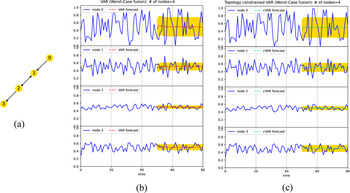
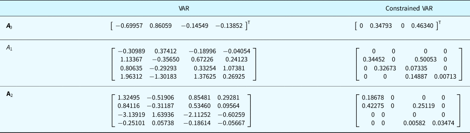
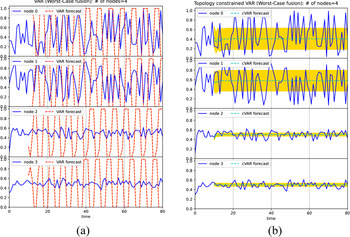
The VAR models are first demonstrated with a four-node-four-edge example in Figure 3a. The simulation data are collected to train the VAR model in Eq. (9) with lag order L = 2. The training is done with the simulation data from the first 50 time steps. The forecast in the next 30 time steps is generated from the VAR model. The same data are used to train the constrained VAR model in Eq. (10). The results are shown in Figure 3b,c respectively, where the solid lines are the simulated probabilities and the dash lines indicate the predictions or forecasts from the models. The shaded regions indicate the predicted error bounds with one standard deviation (±σ). Here the worst-case fusion rule is applied in the simulation. It is seen that the models predict the general trend well. The predictions from the two models are similar. Similar to any other time series models, VAR models focus more on the near-term forecasts. The forecasts of the distant future are more of the average trend. The calibrated coefficients of the two VAR models after training are compared in Table 1. If there is no directed edge connection between nodes, the corresponding coefficients in the constrained VAR model are zeros. Notice that some fitted coefficients in the traditional VAR model have negative values, whereas the ones in the constrained VAR model are all positive with values between zero and one. Since the values of both independent and dependent variables here are probabilities, it is difficult to interpret the negative coefficients. In contrast, the fitted coefficients in the constrained VAR model are associated with the reliance probabilities. They can be interpreted as the conditional probability of positive prediction for a node given its information source. Therefore, the sparser set of parameters in the constrained VAR model provides both efficient and physically meaningful representations. To quantitatively compare the forecast accuracy, mean squared error (MSE), which is the average squared difference between the forecasts and the original data during the forecast period, is calculated. The MSE for the VAR model is 0.02083, whereas the one for the constrained VAR model is 0.02116. Although the coefficients in the constrained VAR model are much sparser and there are only 13 out of 36 coefficients are non-zero, the model still can have the similar performance as in the traditional VAR model.

Fig. 3.

The simulated prediction probabilities and forecast with 50 time steps of training. (a) The four-node-four-edge example; (b) result of the VAR model (MSE = 0.02083); and (c) result of the constrained VAR model (MSE = 0.02116).

Table 1.

Comparison of the calibrated parameters between the VAR model and constrained VAR model in Figure 3 for the four-node-four-edge network

To further demonstrate the training efficiency, fewer training data are applied to the four-node-four-edge example. Only the first 10 steps of simulation data are used to train the VAR models. The results are shown in Figure 4. The traditional VAR model is not fully trained and the predictions become very unstable with the limited training data, whereas the constrained VAR model still predicts reasonably well. The MSEs for the VAR model and constrained VAR model are 0.16667 and 0.03118, respectively.

Fig. 4.

The simulated prediction probabilities and forecast with only 10 time steps of training from (a) the VAR model (MSE = 0.16667) and (b) the constrained VAR model (MSE = 0.03118).

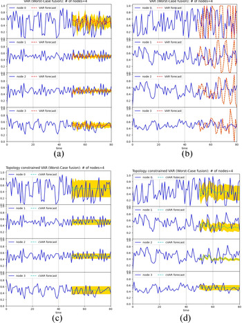
The sensitivity of the model performance with respect to the lag order is tested. The traditional and constrained VAR models with lag orders of L = 6 and L = 12 are constructed. The results are compared in Figure 5. It is seen that higher-order models can provide more details of longer-term predictions instead of average values only. However, the number of model parameters to be fitted also increases. As seen in Figure 5b, the number of coefficients in the traditional VAR model with lag order L = 12 has increased so much that 50 time steps of training data become not enough for model training. In contrast, the constrained VAR model has the reduced number of effective coefficients. As seen in Figure 5d, the model with L = 12 shows good prediction performance.

Fig. 5.

The sensitivity studies of different lag orders. (a) VAR model with L = 6 (MSE = 0.03522); (b) VAR model with L = 12 (MSE = 0.15196); (c) constrained VAR model with L = 6 (MSE = 0.02697); (d) constrained VAR model with L = 12 (MSE = 0.04394).

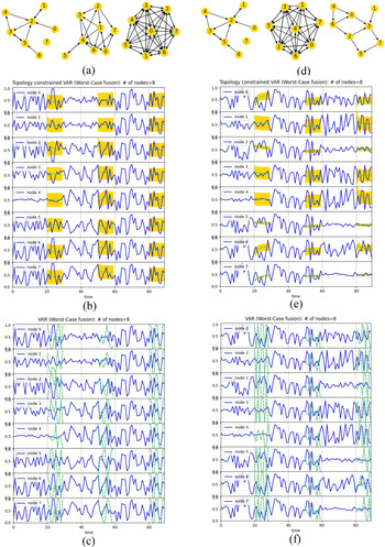
A second example is to demonstrate how data-driven modeling can be applied to dynamic networks where topology changes along time. As shown in Figure 6a, an 8-node network with 10 edges is initially constructed. After 30 time steps, the network topology is changed to 18 edges at the second epoch. The network is further changed to 54 edges during the third epoch. The simulated and forecasted prediction probabilities with the constrained VAR model are shown in Figure 6b, whereas the forecasts by the traditional VAR model are shown in Figure 6c. For each epoch of 30 time steps, the data of the first 20 time steps are used to train the VAR models. The forecasts of the next 10 steps are compared with the simulation data. A different case is shown in Figure 6d, where the numbers of edges change to 43 and 10 during the next two epochs from the same initial 8-node-10-edge network as in Figure 6a. The simulation and forecast results are shown in Figure 6e,f. It is seen that the constrained VAR model predicts the trends reasonably well even with the dynamic topological changes and small training datasets. Dynamically evolving networks may not allow us to collect a large amount of data for training.

Fig. 6.

The dynamic 8-node network with topology changes: (a) 8-node-10-edge network changes to 18 and 54 edges along time; (b) the constrained VAR model (MSE = 0.05563); (c) the VAR model (MSE = 0.20507); (d) 8-node-10-edge network changes to 43 and 10 edges along time; (e) the constrained VAR model (MSE = 0.05997); and (f) the VAR model (MSE = 0.24637).

As also seen in Figure 6, the fluctuation patterns of prediction probabilities vary when the network topology changes, because information sharing patterns are different. When there are more connections, the coupling between nodes becomes stronger. The prediction probabilities tend to fluctuate more and be more synchronized. When a node does not receive information from others, such as nodes 0, 6, and 7 during the first epoch and nodes 1 and 4 during the third epoch in Figure 6d, the prediction can still fluctuate as a result of pure random effects. Some levels of information sharing suppress the fluctuations. Yet fully connected network can amplify the fluctuation with synchronization.

Demonstration of latent variable VAR model

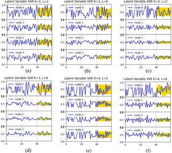
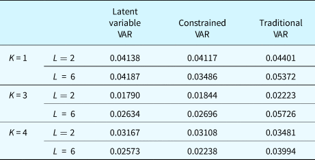
Here the latent variable VAR model is demonstrated. The model is constructed to predict the previous 4-node-4-edge network example in Figure 3a. Different values of factor number K and lag order L in Eqs (12) and (13) are tested. The results are shown in Figure 7. The MSEs of forecasts from the latent variable VAR, topology constrained VAR, and traditional VAR are compared in Table 2. The forecasts by latent variable VAR and constrained VAR are more accurate than those by traditional VAR. Similar to other VAR models, when the lag order increases, the longer-term fluctuation can be predicted. In comparison with Figure 5a for traditional VAR model of lag order L = 6, the results in Figure 7b,d,f with the same lag order are more stable and accurate. Therefore, introducing latent variables helps identify the intrinsic interdependency between observable variables.

Fig. 7.

The latent variable VAR model forecasts for 4-node-4-edge network with different latent variable number K and lag order L. (a) K = 1, L = 2; (b) K = 1, L = 6; (c) K = 3, L = 2; (d) K = 3, L = 6; (e) K = 4, L = 2; (f) K = 4, L = 6.

Table 2.

Comparison of forecast MSEs by the latent variable VAR, constrained VAR, and traditional VAR models

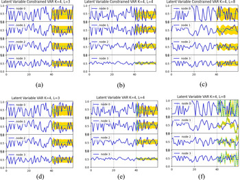
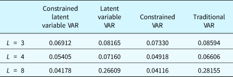
The topology constrained latent variable VAR is further demonstrated with the 4-node-4-edge network example. With the factor number fixed as K = 4, three cases with different lag orders are compared. The results of MSEs from the constrained latent variable VAR model, in comparison with the latent variable VAR, constrained VAR, and traditional VAR, are shown in Table 3. It is seen that the topology constraints can help improve the forecast accuracy for both VAR and latent variable VAR models. The accuracy levels are similar for these two constrained models. The forecasts of the latent variable VAR models with and without topology constraints are also shown in Figure 8. As the lag order increases, the number of coefficients to be trained also increases, which requires more training data. The topology constraints can effectively reduce the number of coefficients and improve the training efficiency with less training data, such as the case when L = 8.

Fig. 8.

The latent variable VAR model forecasts for the 4-node-4-edge network with different lag orders where K = 4. (a) L = 3 with constraints; (b) L = 4 with constraints; (c) L = 8 with constraints; (d) L = 3 without constraints; (e) L = 4 without constraints; (f) L = 8 without constraints.

Table 3.

Comparison of forecast MSEs by constrained latent variable VAR, latent variable VAR, constrained VAR, and traditional VAR with K = 4

Demonstration of spatial–temporal GPR model

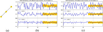
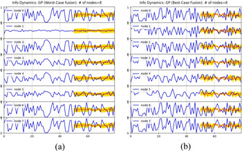
We also implemented and tested the proposed spatial–temporal hybrid GPR time series model to predict the dynamics of prediction probabilities. The results for the 3-node-3-edge example are shown in Figure 9. Two different data fusion rules, worst-case and best-case scenarios, are applied here. The results for the 8-node-10-edge example are shown in Figure 10. Compared to the previous linear VAR models which only predict the general trend in long term, the GPR model predicts the nonlinear dynamics of probabilities better. More fluctuations for both means and variances are observed in the forecasts. This is because of the kernel functions in GPR models which are able to capture differences locally based on the distance metrics. Thus the GPR model provides more details about the long-term dynamics in the networks. The proposed GPR model with the considerations of both spatial and temporal correlations between nodes captures the information dependency between nodes.

Fig. 9.

The simulated prediction probabilities and forecast by the GPR model in the 3-node-3-edge example, with (a) the worst-case fusion rule (MSE = 0.03203), and (b) the best-case fusion rule (MSE = 0.03795).

Fig. 10.

The simulated prediction probabilities and forecast by the GPR model in the 8-node-10-edge example, with (a) the worst-case fusion rule (MSE = 0.03924), and (b) the best-case fusion rule (MSE = 0.05461).

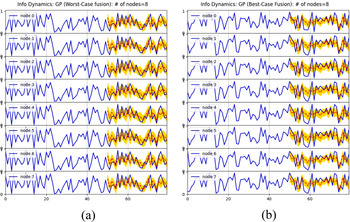
When all 8 nodes in the network are fully connected, the simulation and forecast results of the 8-node-56-edge example are shown in Figure 11. Because each node is connected with all other nodes, very strong correlations exist in the fully connected network. It is seen that the prediction probabilities of all nodes are synchronously fluctuating with the same values after a short period. The GPR model also predicts the synchronized fluctuations with error bounds.

Fig. 11.

The simulated prediction probabilities and forecasts by the GPR model in the 8-node-56-edge example, with (a) the worst-case fusion rule (MSE = 0.06174), and (b) the best-case fusion rule (MSE = 0.08055).