2. Numerical approach

In recent studies, the lattice Boltzmann method has been used for eddy-resolving simulations of turbulent flows in complicated geometries, such as flows in porous media (Chukwudozie & Tyagi Reference Chukwudozie and Tyagi2013; Kuwata & Suga Reference Kuwata and Suga2015; Fattahi et al. Reference Fattahi, Waluga, Wohlmuth, Rüde, Manhart and Helmig2016) and flows over porous walls (Kuwata & Suga Reference Kuwata and Suga2016a, Reference Kuwata and Suga2017), rough walls (Kuwata & Kawaguchi Reference Kuwata and Kawaguchi2018a, Reference Kuwata and Kawaguchi2019) and urban canopy (Onodera et al. Reference Onodera, Aoki, Shimokawabe and Kobayashi2013; Lenz et al. Reference Lenz, Schoenherr, Geier, Krafczyk, Pasquali, Christen and Giometto2019), because of its advantages such as simplicity of the wall treatment, high spatial locality of the calculations and high accuracy resulting from low numerical dissipation and dispersion. For 3-D simulations using the lattice Boltzmann method, several possible alternatives can be used for discrete velocity and collision models. In this study, we employed the D3Q27 multiple-relaxation-time lattice Boltzmann method for the flow fields, which was rigorously validated by conducting eddy-resolving simulations of a turbulent channel flow, a pipe flow, a duct flow and porous medium flows (Suga et al. Reference Suga, Kuwata, Takashima and Chikasue2015), and has been successfully applied to turbulent flows over porous and rough walls (Kuwata & Suga Reference Kuwata and Suga2016a, Reference Kuwata and Suga2017; Kuwata & Kawaguchi Reference Kuwata and Kawaguchi2018a,Reference Kuwata and Kawaguchib). For the scalar fields, we employed the D3Q19 model with regularization procedures. The regularization procedure proposed by Latt & Chopard (Reference Latt and Chopard2006) projects the non-equilibrium distribution function onto the Hermite polynomial, which greatly improves the accuracy and numerical stability, and has been successfully applied to the DNSs of turbulent heat transfer in complex geometries (Suga, Chikasue & Kuwata Reference Suga, Chikasue and Kuwata2017; Nishiyama, Kuwata & Suga Reference Nishiyama, Kuwata and Suga2020).

3. Flow configuration and computational details

3.1. Flow geometry and boundary conditions

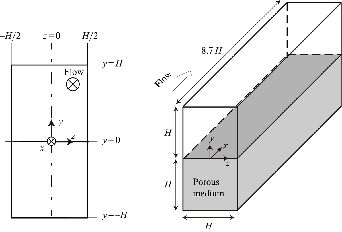
Figure 1 illustrates the configuration of a rectangular duct flow partially filled with a porous material. This flow system is comparable to that employed in the experimental study of Suga et al. (Reference Suga, Okazaki and Kuwata2020). The rectangular duct size ($L_x(x) \times L_y(y) \times L_z (z)$) is $8.7H(x) \times 2H(y) \times H(z)$ in the streamwise, vertical and horizontal directions, respectively. A porous medium consisting of staggered square bar arrays is considered in the bottom half of the rectangular duct $-1<y/H<0$; hence, the cross-section of the clear flow region is $H(y) \times H(z)$. Periodic boundary conditions are applied in the streamwise direction, and the flow is driven by a streamwise pressure difference. To ensure the no-slip boundary conditions at the duct walls and surfaces of the porous medium, the half-way bounce-back method is applied to the distribution function. The Reynolds number based on the bulk mean velocity in the clear fluid region, $U_b$, and the duct width, $H$, is 3500. For the thermal boundary conditions, the top ($y=H$) and bottom ($y=-H$) walls are considered to be isothermal with a temperature difference $\Delta T$ ($\Delta T>0)$, and $T_{y=H}=T_{y=-H}+\Delta T$, whereas the lateral walls at $z=-0.5H, 0.5H$ are considered as adiabatic walls. The conjugate heat transfer conditions are applied to the porous medium, and the heat conduction of the porous material is simultaneously solved considering the thermal energy interaction between the solid and fluid phases. The fluid Prandtl number is set to $Pr=0.71$, and the ratio of the thermal diffusivity of the solid phase to that of the fluid phase is $4.4$, assuming airflow thorough an aluminium porous material. The study by Yoshida & Nagaoka (Reference Yoshida and Nagaoka2010) can be referred to for implementation of the adiabatic and isothermal boundary conditions, while the study of Wang, Wang & Li (Reference Wang, Wang and Li2007) can help in understanding the conjugate heat transfer conditions in the framework of the lattice Boltzmann method. Note that the buoyancy effect is crucial in a turbulent square duct flow because the secondary flow pattern under the buoyancy effect entirely differs from that without the effect (Sekimoto et al. Reference Sekimoto, Kawahara, Sekiyama, Uhlmann and Pinelli2011). However, as a first step towards understanding the porous wall effects in 3-D flow systems, this study assumed a passive scale neglecting the buoyancy effect.

Figure 1.

Sketch of a configuration of a porous duct flow.

3.2. Porous medium characteristics and averaging procedure

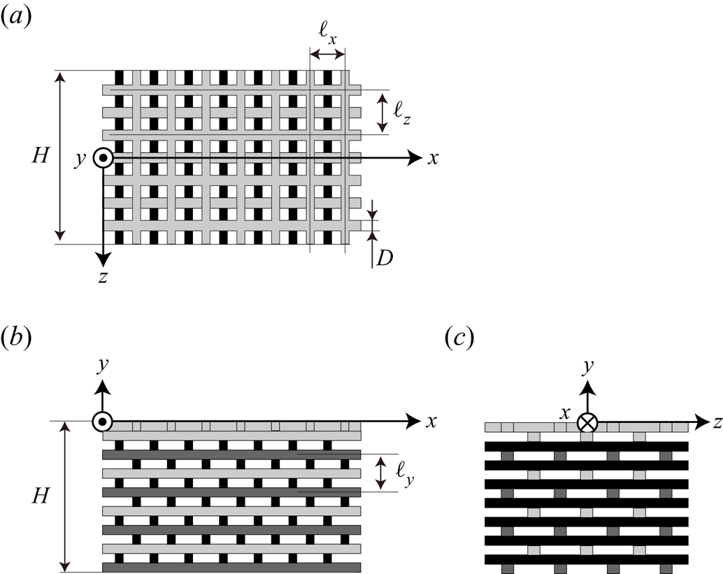
The geometry of the porous medium under consideration is identical to that used in the experimental study of Suga et al. (Reference Suga, Okazaki and Kuwata2020), as shown in figure 2. As can be seen, the porous medium is comprised of square bars of size $D/H=6.00\times 10^{-2}$, and the distance between the bar centres is $\ell _x/D=\ell _z/D=4.33$. The porosity of the porous medium is $\varphi =0.77$. This porous medium is an orthogonal porous medium because the pressure gradient along the $i$ axis, ${\partial P}/{\partial x_i}$, only drives the volume-averaged velocity component in the $i$ direction, $U_i$, i.e. the off-diagonal components of the permeability tensor are zero, $K_{ij}=0$ ($i\neq j$). The permeability tensors were measured in the fully developed flows in the duct filled by the porous medium. The streamwise, vertical and horizontal components of the permeability tensor were obtained from the flow rate and pressure drops using the Darcy–Forchheimer equation (Whitaker Reference Whitaker1986); the values measured by Suga et al. (Reference Suga, Okazaki and Kuwata2020) were $K_{xx}/H^2 = 7.6 \times 10^{-5}$, $K_{yy}/H^2 = 6.0 \times 10^{-5}$ and $K_{zz}/H^2 = 7.6 \times 10^{-5}$, respectively.

Figure 2.

Geometry of a porous medium. $(a)$ Top view, $(b)$ side view and $(c)$ front view.

In the following discussion, the variables in the clear flow region ($y>0$) are averaged over time and in the streamwise direction, while for those in the porous medium region ($y<0$), intrinsic line averaging (phase averaging) is conducted in the streamwise direction. Thus, the fluid-phase variables are averaged over a fluid-phase line segment whereas the solid ones are averaged over a solid-phase line segment as follows:

(3.1a,b)\begin{equation} {[\phi_f]} = \frac{1}{\Delta L_{f} }\int_{x} \phi_f\, \textrm{d}\,L_{f}, \quad {[\phi_s]} = \frac{1}{L_{s}}\int_{x} \phi_s \,\textrm{d}L_{s}, \end{equation}

where subscripts ‘$f$’ and ‘$s$’ denote the variables for the fluid and solid phases, respectively; $L_f$ and $L_s$ are the streamwise line segments of fluid and solid phases: $L_x=L_f+L_s$. It is noted that, near the porous wall, the averaging over the streamwise direction does not coincide with the Reynolds averaging because the structure of the porous medium under consideration is inhomogeneous in the streamwise direction.

When we statistically discuss heat and fluid flow in the porous medium region with a macroscopic viewpoint, volume averaging carried out over the representative elementary volume (REV) is introduced as follows:

(3.2a,b)\begin{equation} {\langle \phi_f \rangle} = \frac{1}{\Delta V_f}\int_{V_f} \phi_f \,\textrm{d}V_f, \quad {\langle \phi_s \rangle} = \frac{1}{\Delta V_s}\int_{V_s} \phi_s \,\textrm{d}V_s, \end{equation}

where the size of the REV is defined as $\ell _x (x) \times \ell _y (y) \times \ell _z (z)$ in figure 2; thus, the volume of the REV is $\Delta V=\Delta V_f+\Delta V_s=\ell _x \ell _y \ell _z$. It is noted that the REV is the smallest volume for which the characteristic parameters of the porous medium (porosity and permeability tensor) are independent of the size; thus, a relation exists as $\varphi =\Delta V_f/\Delta V$.

In the following discussion, the Reynolds-averaged value of a variable $\phi$ is denoted by $\bar {\phi }$, and $\phi '$ denotes the fluctuation from the Reynolds-averaged value: $\phi ' = \phi -\bar {\phi }$. For the Reynolds averaging, the simulation is run for $209T$ (where $T=H/U_b$ is the convection time), after the flow has reached a fully developed state. The dispersion from the volume-averaged (phase-averaged) value over the REV is denoted as $\tilde {\phi } = \phi -{\langle \phi \rangle }$.

3.3. Computational details

This study uses the uniform spacing grid $3328(x) \times 770(y) \times 386(z)$ for $8.7H(x) \times 2H(y) \times H(z)$, which corresponds to a cross-section of a square bar being resolved by $23\times 23$ grids. To assess the grid independence of the solutions, we performed additional simulation with twofold coarser resolution grids, and found no perceptible change in the simulation results (the difference in the maximum peak value of the turbulence intensity was confirmed to be approximately 1 %). Moreover, the grid spacing in wall units is confirmed to be approximately 1.0, which is much finer than those used in lattice Boltzmann DNS studies (Kuwata & Suga Reference Kuwata and Suga2016a, Reference Kuwata and Suga2017; Kuwata & Kawaguchi Reference Kuwata and Kawaguchi2018a; Kuwata & Suga Reference Kuwata and Suga2019). Note that the wall unit, $\nu /u_{\tau p}$, is defined with the kinematic viscosity $\nu$ and averaged friction velocity $u_{\tau p}$ at the porous wall as given in § 4.

In terms of the computational domain length, since the computational domain length presently used, $L_x=8.7H$, is longer than that employed in the numerical simulations of square duct flows by Huser & Biringen (Reference Huser and Biringen1993), Madabhushi & Vanka (Reference Madabhushi and Vanka1991) and Zhang et al. (Reference Zhang, Trias, Gorobets, Tan and Oliva2015), the domain length is expected to be sufficient to capture turbulent vortex motion. Nonetheless, it should be noted that there is still much controversy about the sufficient domain length for square duct flows (Vinuesa et al. Reference Vinuesa, Noorani, Lozano-Durán, Khoury, Schlatter, Fischer and Nagib2014).

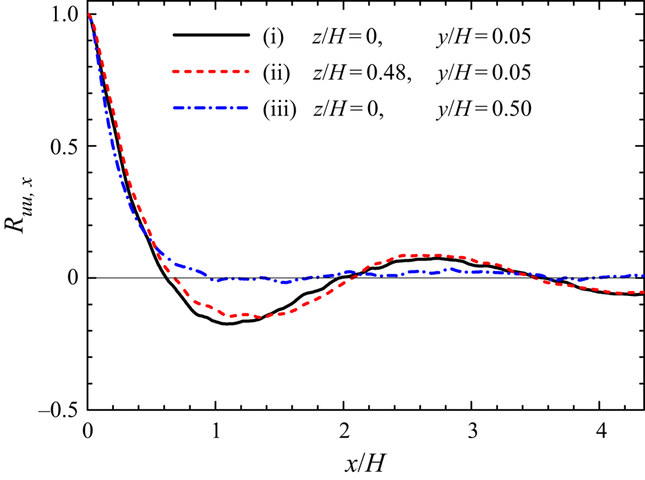
For the porous wall turbulence, it is well established that the large-scale streamwise perturbation arising from the K–H instability develops over the permeable porous wall (Finnigan Reference Finnigan2000; Jimenez et al. Reference Jimenez, Uhlmann, Pinelli and Kawahara2001), and requires a longer streamwise domain length compared to that used in smooth-wall-bounded turbulent flow simulations (Kuwata & Suga Reference Kuwata and Suga2016a, Reference Kuwata and Suga2017, Reference Kuwata and Suga2019). Hence, as seen in figure 3, we examine the two-point spatial correlation function $R_{uu,x}$ of streamwise velocity fluctuations at several locations to validate the domain length.

Figure 3.

Two-point spatial correlation function of streamwise velocity fluctuations at three ($y,z$) locations: (i) a profile over the porous medium in the symmetry plane, (ii) a profile near the corner over the porous medium and (iii) a profile at the centre of the clear flow region.

It is observed that over the porous medium, profiles of $R_{uu,x}$ in cases (i) and (ii) are wavy, and exhibit local minimum points at $x/H \simeq 1.2$. This observation suggests the presence of large-scale streamwise perturbation in the duct flow system arising from the K–H instability, which is consistent with the results of the experimental study of Suga et al. (Reference Suga, Okazaki and Kuwata2020). Suga et al. (Reference Suga, Okazaki and Kuwata2020) reported that the streamwise perturbation could develop in the porous duct flow despite the confinement by the lateral walls. Similarly in this study, the profile near the corner (case (i)) over the porous medium was very close to the one in the symmetry plane (case (ii)), thus indicating that the K–H waves are not reduced by the lateral walls. 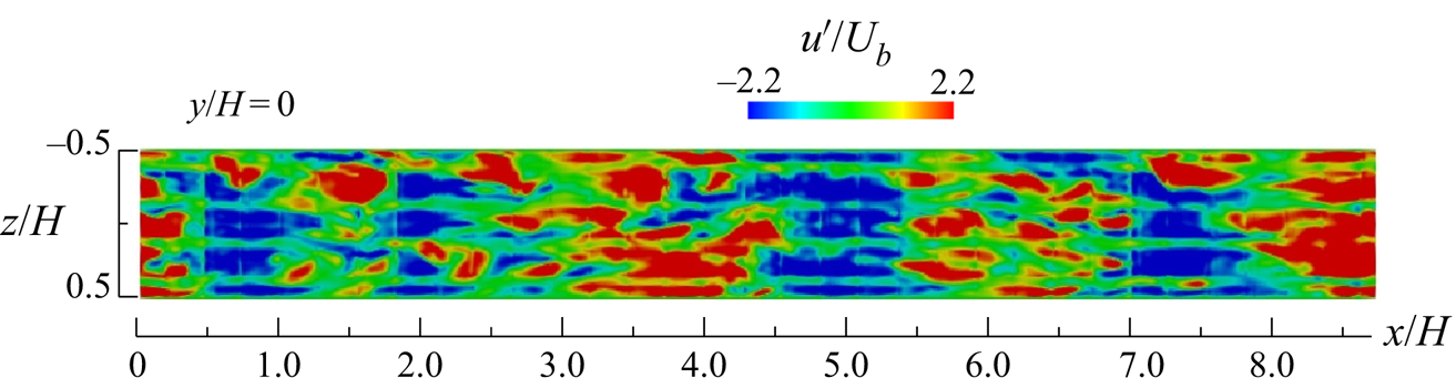The presence of the streamwise perturbation is also confirmed from a snapshot of streamwise velocity fluctuations just above the porous–fluid interface at $y/H=0.0013$, as seen in figure 4. It is observed that the high- and low-speed regions, which have strong coherence in the spanwise direction, alternately appear in the streamwise direction (see Kuwata & Suga (Reference Kuwata and Suga2016a, Reference Kuwata and Suga2019) for detailed discussions of the turbulence structure associated with the K–H instability in the porous-walled channel). Figure 3 confirms that the magnitude in $R_{uu,x}$ falls below 0.1 at half the domain length but does not not completely converge to zero. To ensure the computational domain size, we further performed a domain size test with a domain size twice as large in the streamwise direction, yielding a 2 % difference in the maximum peak of the turbulence energy.

Figure 4.

Snapshot of streamwise turbulent velocity fluctuations in the $x$–$z$ plane just above the porous–fluid interface at $y/H=0.0013$.

3.4. Validation

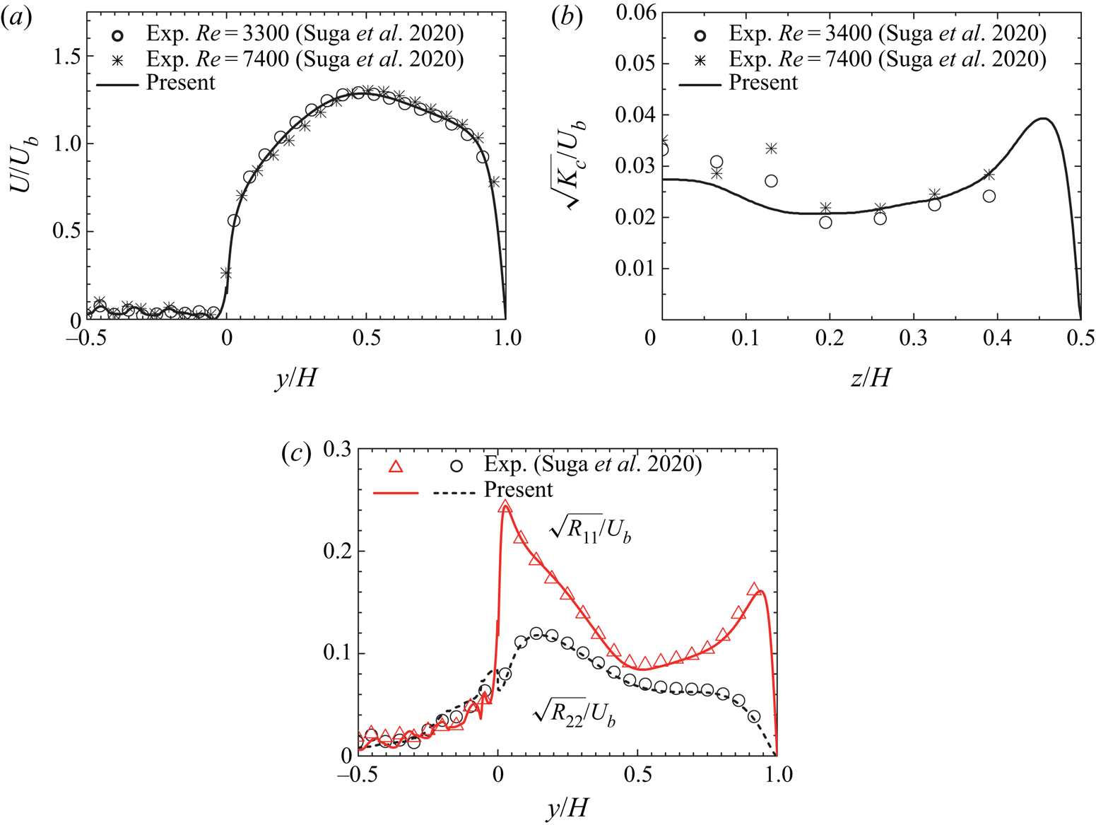
This subsection provides validation of the present numerical method through a comparison of the turbulence statistics with the experimental data from Suga et al. (Reference Suga, Okazaki and Kuwata2020) and DNS data from Samanta et al. (Reference Samanta, Vinuesa, Lashgari, Schlatter and Brandt2015). Figure 5 presents comparisons of the turbulence statistics with the experimental data. Following Suga et al. (Reference Suga, Okazaki and Kuwata2020), the mean velocity in figure 5(a) and the Reynolds stresses in figure 5(c) are averaged over $-\ell _z/2 < z < \ell _z/2$, and the kinematic energy of the secondary flow intensity in figure 5(b) is averaged over $0<y<H$. It is shown that the mean velocity in figure 5(a) and the kinetic energy of the secondary flow in figure 5(b) do not strongly depend on the Reynolds number. The skewed mean velocity profile with respect to $y/H=0.5$ collapses onto the experimental data in figure 5(a), and the enhanced kinetic energy of the secondary flow in comparison with the square duct flow (Suga et al. Reference Suga, Okazaki and Kuwata2020) is reasonably predicted in figure 5(b). The enhancement of the turbulence over the porous wall is perfectly reproduced in figure 5(c). Moreover, figure 5(c) also shows that the turbulence intensities in the porous medium region $y<0$ generally agree with the experimental data. Thus, it can be concluded that the present method can accurately reproduce turbulence inside the porous medium region.

Figure 5.

Comparison of the predicted turbulence statistics with the experimental data from Suga et al. (Reference Suga, Okazaki and Kuwata2020). $(a)$ Streamwise mean velocity, $(b)$ kinematic energy of secondary flow and $(c)$ Reynolds stresses. The mean velocity and the Reynolds stresses are averaged over $-\ell _z/2 < z < \ell _z/2$: $U=\int _{-\ell _z/2}^{\ell _z/2} {[\bar {u}]}\,\textrm {d}z/{\ell _z}$ and $R_{ij}=\int _{-\ell _z/2}^{\ell _z/2} {[ \overline {u'_i u'_j}]}\,\textrm {d}z/{\ell _z}$. The kinematic energy of secondary flow is averaged over $0<y<H$: $K_c= \int _{0}^{H} ({[\bar {v}]}^2 + {[ \bar {w} ]}^2 )\,\textrm {d}y/{H}$. Note that the porous medium for the results of $K_c$ from Suga et al. (Reference Suga, Okazaki and Kuwata2020) is not identical to that employed in this study.

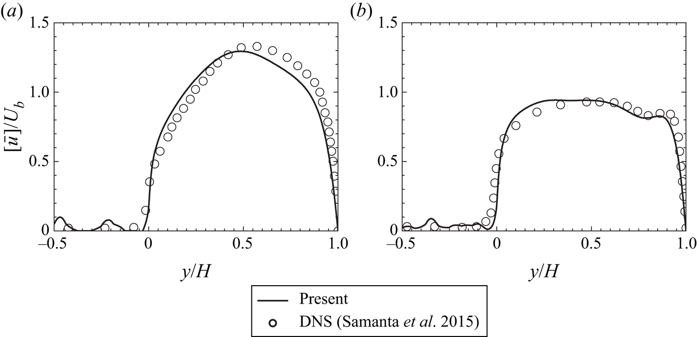
Figure 6 presents comparisons of the predicted mean velocity with the DNS data of the porous duct flow at $Re_b=5500$ from Samanta et al. (Reference Samanta, Vinuesa, Lashgari, Schlatter and Brandt2015). It should be noted that direct comparison of the simulation results may not be possible because of the difference in the characteristics of the porous medium and the simulated Reynolds number. Moreover, the DNS study of Samanta et al. (Reference Samanta, Vinuesa, Lashgari, Schlatter and Brandt2015) did not resolve the porous geometry, but only solved the volume-averaged equations with the drag force model of Whitaker (Reference Whitaker1996) and Breugem et al. (Reference Breugem, Boersma and Uittenbogaard2006). Nevertheless, the general trend of the mean velocity profile at $z/H=0.0$ and $0.45$ appears qualitatively similar. Therefore, the findings of the present study are not limited to the case with this specific porous medium geometry and Reynolds number, and the conclusions obtained in this study can be generalized for other scenarios.

Figure 6.

Comparison of the mean velocity profile with the DNS results from Samanta et al. (Reference Samanta, Vinuesa, Lashgari, Schlatter and Brandt2015): $(a)$ at $z/H=0.0$ and $(b)$ at $z/H=0.45$.

4. Wall shear stress and wall heat flux

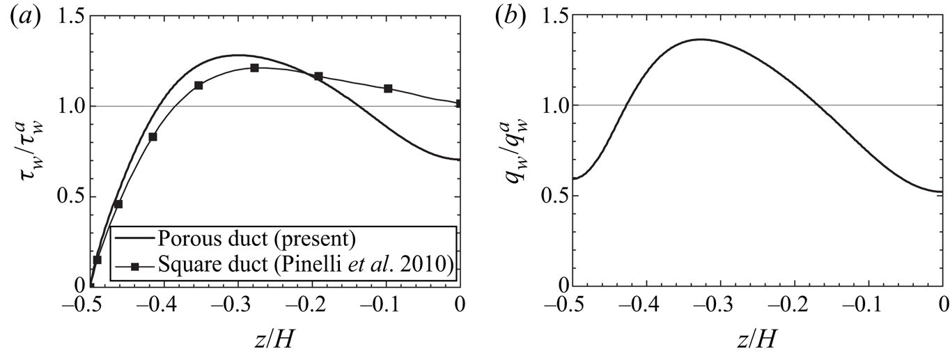
Before discussing the detailed flow physics, this section concentrates on the global flow characteristics, including the skin friction coefficient and the Nusselt number. Figure 7 presents profiles of the wall shear stress $\tau _w/\tau _w^a$ and wall heat flux $q_w /q_w^a$ at the top wall $y/H = 1.0$. Here, $\tau _w^a$ and $q_w^a$ denote the averaged values over the top wall. For comparison, the square duct DNS result of $\tau _w/\tau _w^a$ from Pinelli et al. (Reference Pinelli, Uhlmann, Sekimoto and Kawahara2010) at $Re_b=3600$ (based on the duct width $H$) is included. Figure 7(a) confirms that the profile of $\tau _w/\tau _w^a$ for the square duct flow takes a local maximum value around $z/H=-0.26$ and a minimum value at the symmetry plane, which is associated with the presence of a low-velocity streak flanked by two high-velocity ones near the wall (Pinelli et al. Reference Pinelli, Uhlmann, Sekimoto and Kawahara2010). For the porous duct flow, the wall shear stress takes a maximum peak value at around $z/H = -0.3$, but it rapidly decreases as it approaches the middle of the top wall $z/H = 0.0$. The maximum peak value of $\tau _w/\tau _w^a$ for the porous duct is approximately 6 % larger than that for the square duct whereas the local minimum value is 31 % smaller, indicating that non-uniformity of $\tau _w$ due to the lateral walls is more substantial for the porous duct. As in the case of the wall shear stress, the wall heat flux in figure 7(b) exhibits a maximum peak value at around $z/H = -0.3$ and it decreases towards the midpoint at $z/H = 0.0$. The maximum peak value of $q_w/q_w^a$ is found to be 6 % larger than that of $\tau _w/\tau _w^a$, and the reduction of $q_w/q_w^a$ is more notable in the symmetry plane.

Figure 7.

$(a)$ Wall shear stress profile at the top wall and $(b)$ wall heat flux profile at the top wall. The DNS data of square duct flow from Pinelli et al. (Reference Pinelli, Uhlmann, Sekimoto and Kawahara2010) are included.

The bulk wall shear stress at the porous–fluid interface $\tau _{wp}^a$ is computed from the momentum balance between the pressure drop $\Delta P$ and the wall shear stress in the clear flow region ($y>0.0$) as follows:

(4.1)\begin{equation} \Delta P H^2 = 3HL_x\tau_{ws}^a + HL_x\tau_{wp}^a, \end{equation}

where the bulk wall shear stress at the solid wall $\tau _{ws}^a$ is given as

(4.2)\begin{equation} \tau_{ws}^a = \frac{1}{3H} \left( \int_0^H\tau_w \mid_{z=-H/2}\,\textrm{d}y + \int_0^H\tau_w \mid_{z=H/2}\,\textrm{d}y + \int_{-H/2}^{H/2} \tau_w \mid_{y=H}\,\textrm{d}z \right). \end{equation}

This yields the bulk friction velocity at the porous wall, $u_{\tau p} = \sqrt {\tau ^a_{wp}/\rho }$, as follows:

(4.3)\begin{equation} u_{\tau p} = \sqrt{ \frac{1}{\rho} \frac{H\Delta P}{L_x}-3\frac{\tau_{ws}^a}{\rho}}. \end{equation}

The friction Reynolds number for the porous wall is $Re_\tau ^p = u_{\tau p}h/\nu =197$ and that for the top wall is $Re_\tau ^s = u_{\tau s}h/\nu =135$, with $u_{\tau s} = \sqrt {\tau_{ws}^a/\rho }$ and $h$ being the half-duct size, $h=0.5H$. This confirms that the bulk wall shear stress at the porous wall is thus $2.1$ times larger than that at the solid walls: $\tau _{wp}^a/\tau _{ws}^a=2.1$. The permeability Reynolds number, $Re_K=\sqrt {K}u_{\tau p}/\nu$, is $Re_K=3.4$ with $K$ being the mean permeability, $K=K_{ii}/3$. This value is comparable to that in the DNS of porous-walled turbulent channel flow of Kuwata & Suga (Reference Kuwata and Suga2016a) where the turbulence over the porous medium is significantly enhanced due to the effects of wall permeability. The Nusselt number representing the heat transfer rate in the clear flow region is given by the temperature difference in the clear flow region, $\Delta T_c$, and the clear duct height, $H$, according to the following expression: $Nu_c = q_w^a H/(k_f \Delta T_c)$, where $k_f$ is the thermal conductivity for the fluid phase and $\Delta T_c$ denotes the averaged temperature difference between the porous–fluid interface and the top wall. This is computed as $Nu_c = 8.3$. By contrast, the Nusselt number representing the heat transfer rate in the porous medium region is given by the temperature difference in the porous medium region, $\Delta T_p$, and the porous medium height, $H$, according to the following expression: $Nu_p = q_w^a H/(k_{eff} \Delta T_p)$, where $k_{eff}$ is the effective thermal diffusivity, i.e. $k_{eff} = k_f \varphi + k_s (1-\varphi )$ with $k_s$ being the thermal conductivity of the solid phase, and $\Delta T_p$ denotes the averaged temperature difference between the porous–fluid interface and the bottom wall. The value of $Nu_p$ is 1.0, which is significantly smaller than that of $Nu_c$. The reason for this is that the turbulent motion is enhanced over the porous medium but reduced in the porous medium. Hence, the turbulent heat transfer inside the porous medium region is significantly attenuated (see § 10 for a detailed discussion of the heat transfer mechanism).

5. Mean velocity

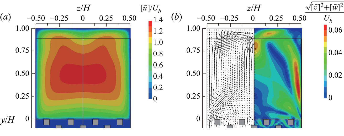
It is well established that the secondary mean flow of the second kind (Prandtl Reference Prandtl1926) is induced by turbulent motion, which is relatively weak but plays a significantly important role in the transport process near corners (Gavrilakis Reference Gavrilakis1992; Huser & Biringen Reference Huser and Biringen1993; Adrian & Marusic Reference Adrian and Marusic2012). Hence, this section first focuses on the modification of this secondary flow pattern due to the presence of the permeable porous wall. 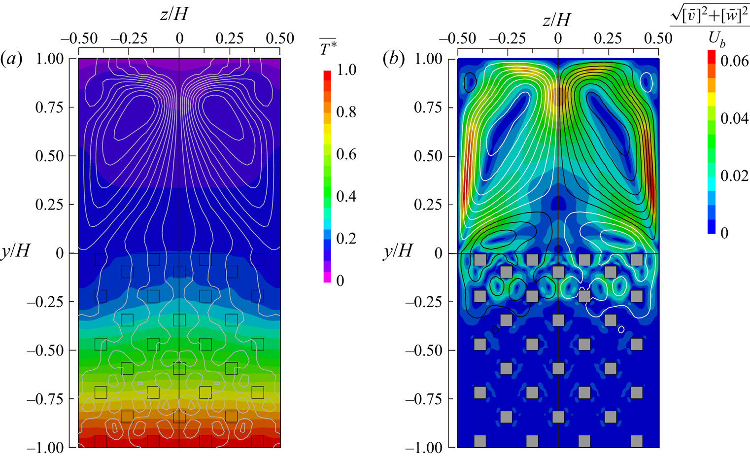Figure 8 presents contour maps of the streamwise mean velocity ${[\bar {u}]}/U_b$ and the secondary flow intensity $\sqrt {{[\bar {v}]}^2+{[\bar {w}]}^2}/U_b$, along with the cross-streamwise mean velocity vectors. In a regular square duct flow, the secondary mean flow is directed towards the corners, and induces eight counter-rotating vortices near these corners (Huser & Biringen Reference Huser and Biringen1993). In contrast, for the porous duct flow, it is observed in figure 8(b) that these eight counter-rotating vortices are absent, and a quite different secondary flow pattern is formed. The secondary flow directed towards the corners above the porous wall can penetrate the porous medium region due to the wall permeability but is also partially blocked by the porous medium. The blocked cross-sectional flow results in upward flow along the lateral walls, and also generates a rotating flow over the porous wall with cores located at $y/H=0.07, z/H=\pm 0.27$. The blocking of the secondary flow by the porous medium generates a global mean flow current in the clear flow region, which is characterized by upward flow along the lateral wall and downward flow in the symmetry plane at $z/H=0$. Moreover, this mean flow current disturbs the corner flow directed towards the top corners, and prevents formation of the counter-rotating vortex pairs near these top corners. This secondary flow pattern is quite similar to that in the DNS study of Samanta et al. (Reference Samanta, Vinuesa, Lashgari, Schlatter and Brandt2015) despite the difference in characteristics of simulated Reynolds number and the porous medium, and complements the view made in the experiments by Suga et al. (Reference Suga, Okazaki and Kuwata2020) who did not confirm the presence of the small recirculating bubbles formed near the top and bottom corners in the clear flow region in figure 8(b). The secondary flow intensity attains a maximum value near the lateral wall, 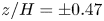$z/H=\pm 0.47$. The maximum peak value is approximately 6 % of the bulk mean velocity, which is considerably larger than that seen in the square duct flow (2 %) (Gavrilakis Reference Gavrilakis1992), but is close to the experimental data of Suga et al. (Reference Suga, Okazaki and Kuwata2020). The enhanced secondary flow may be attributed to two porous medium effects: one is the enhanced turbulent motion due to the relaxation of the wall-blocking effects (Breugem et al. Reference Breugem, Boersma and Uittenbogaard2006; Suga et al. Reference Suga, Matsumura, Ashitaka, Tominaga and Kaneda2010) and the other is low-viscous dissipation at the porous–fluid interface (Samanta et al. Reference Samanta, Vinuesa, Lashgari, Schlatter and Brandt2015).

Figure 8.

Contour maps of the mean velocity. $(a)$ Streamwise mean velocity and $(b)$ secondary flow intensity with the cross-streamwise mean velocity vectors.

The streamwise mean velocity contour in figure 8(a) is only slightly directed towards the corners above the porous wall, as the secondary flow convects the high-momentum fluid towards these corners. On the other hand, in the top half of the clear flow region ($y/H>0.5$), the distortion of the streamwise velocity iso-lines is more prominent. It is observed that the downward secondary flow near the symmetry plane considerably convects the near-wall low-momentum fluid towards the core region, which substantially accelerates the core flow as reported by Samanta et al. (Reference Samanta, Vinuesa, Lashgari, Schlatter and Brandt2015). The detailed momentum transport mechanism is further discussed in § 7.

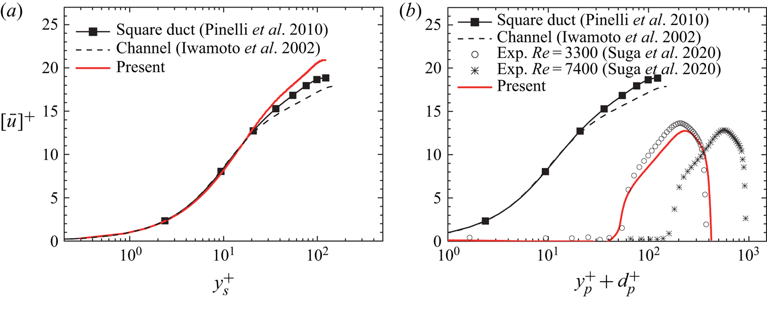
To gain insights into the scaling of the streamwise mean velocity in the clear flow region, an inner-scaled mean velocity profile in a log–linear format is discussed. Figure 9(a) displays a mean velocity profile normalized by the local friction velocity at the middle of the top wall, $z/H=0.0$, $y/H=1.0$, with the top wall coordinate. Also shown are the DNS results in a turbulent channel flow at a comparable Reynolds number of $Re_\tau =150$ from Iwamoto, Suzuki & Kasagi (Reference Iwamoto, Suzuki and Kasagi2002) and for a square duct flow at $Re_\tau =123$ from Pinelli et al. (Reference Pinelli, Uhlmann, Sekimoto and Kawahara2010). The superscript ‘$+$’ stands for scaling with the corresponding viscous length. In figure 9(a), the profiles in the viscous sublayer $y_s^+<10$, with $y_s$ being the distance from the top wall, are consistent in all cases. In the region of $y_s^+>50$, although the logarithmic region is not evident due to the low-Reynolds-number effects, the slopes in the porous duct and square duct flows appear to be somewhat larger than that in the channel flow. In particular, the profiles in the porous duct flow further deviate from the square duct result as it separates from the top wall, which is principally due to the significantly enhanced secondary flow in the symmetry plane.

Figure 9.

Inner-scaled streamwise mean velocity in the log–linear format. $(a)$ Profile near the top wall and $(b)$ profile over the porous medium. The DNS data of turbulent channel flow from Iwamoto et al. (Reference Iwamoto, Suzuki and Kasagi2002) and square duct flow from Pinelli et al. (Reference Pinelli, Uhlmann, Sekimoto and Kawahara2010) are included. The experimental data of porous-duct flows from Suga et al. (Reference Suga, Okazaki and Kuwata2020) are shown in $(b)$.

A profile over the porous medium is discussed by introducing the modified log-law profile:

(5.1)\begin{equation} {\left[ \bar{u} \right]}^{+} = \frac{1}{\kappa} \ln \left ( \frac{y_p^++d_p^+}{h_r^{+}} \right), \end{equation}

where parameters $\kappa$, $d_p$ and $h_r$ are, respectively, the Kármán constant, the zero-plane displacement and the equivalent roughness height. (See Breugem et al. (Reference Breugem, Boersma and Uittenbogaard2006) or Suga et al. (Reference Suga, Matsumura, Ashitaka, Tominaga and Kaneda2010) for the procedure to obtain these parameters.) The normal distance from the porous–fluid interface is denoted as $y_p$. The friction velocity at the porous–fluid interface $y/H=0.0, z/H=0.0$ is evaluated via the total stress at the interface averaged over $-\ell _z/2 < z < \ell _z/2$: $\mu ({\partial {[\bar {u}]}}/{\partial y}) - \rho {\left [ \bar {u} \ \bar {v} \right ]} - \rho {\left [ \overline {u'v'} \right ]}$. Here, $\mu$ is the dynamic viscosity. Figure 9(b) presents the mean velocity profile over the porous wall. The first notable observation is that the slope of the logarithmic region for the porous duct is considerably steeper than that for the channel and square duct flows. In addition, as in the porous-walled turbulent channel flow, the mean velocity profile shifts rightward due to an increase in the mean velocity penetration, and shifts downward due to an increase in skin friction drag. The predictive result shows reasonable agreement with the experimental data at $Re=3300$ from Suga et al. (Reference Suga, Okazaki and Kuwata2020), and the mean velocity at $Re=7400$ shifts rightward due to the increase in the flow penetration while the slope of the profile is not affected by the Reynolds number. The Reynolds number dependence of the log-law parameters is further discussed in Suga et al. (Reference Suga, Okazaki and Kuwata2020) and they stated that the log-law parameters could be reasonably scaled in a fashion similar to that in the case of turbulent porous-walled channel flow. This is supported by the present result that the secondary flow intensity that is averaged over the bottom half of the symmetry plane in the clear flow region is small, 0.9 % of $U_b$. However, it is still larger than the one in the square duct flow. The maximum value of the secondary flow intensity in the symmetry plane is approximately three times larger than the result for a square duct flow from Pinelli et al. (Reference Pinelli, Uhlmann, Sekimoto and Kawahara2010). This suggests that the influence of the lateral walls in the symmetry plane is not significant but still larger than that in the square duct flow.

6. Turbulence intensities

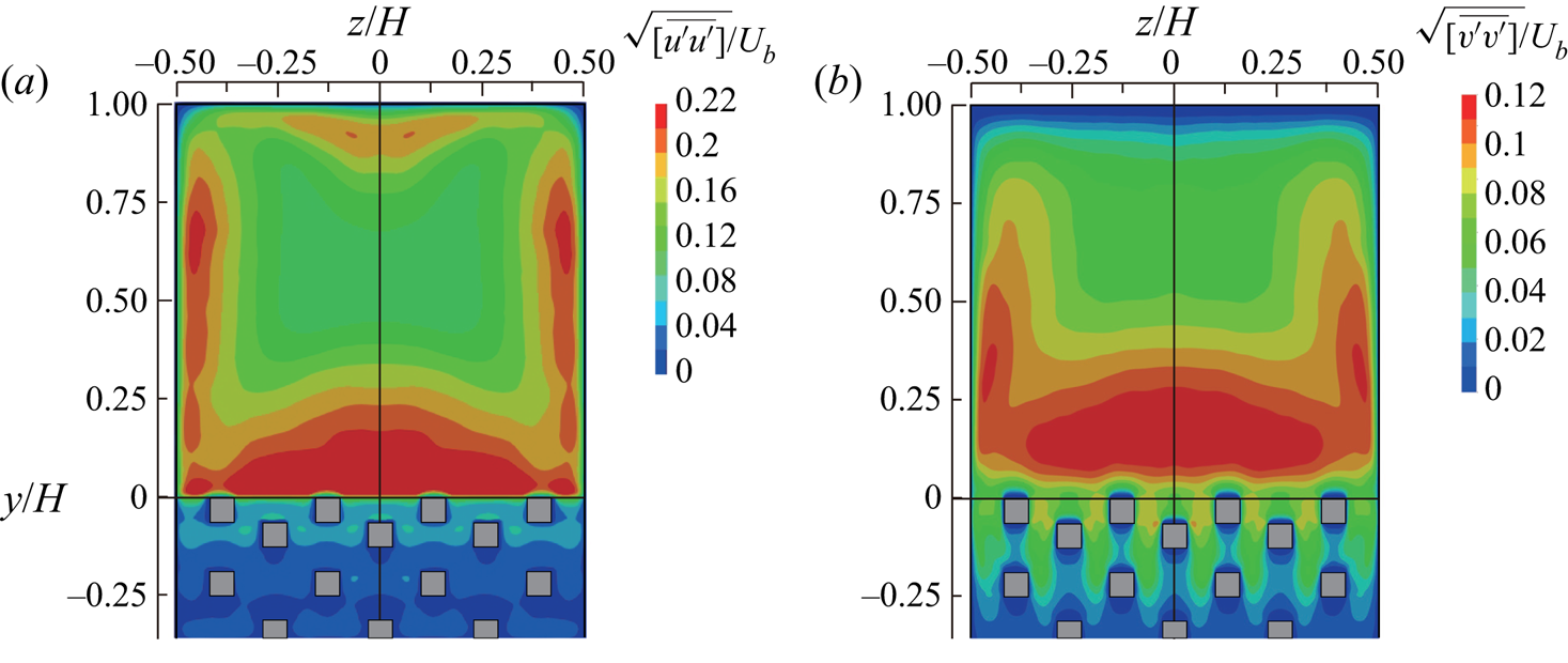
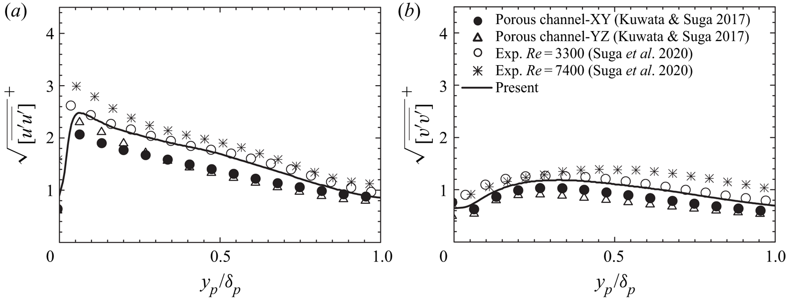
This section briefly reviews the 3-D effects due to the presence of the lateral walls on the turbulence intensity. Figure 10 presents contour maps of the streamwise and vertical turbulence intensities $\sqrt {{[\overline {u'^2}]}}$ and $\sqrt {{[\overline {v'^2}]}}$, both of which are normalized by the bulk mean velocity. It is evident from the figure that turbulence over the porous wall is enhanced considerably, which is consistent with the observations in the porous-walled turbulent channel flows (Breugem et al. Reference Breugem, Boersma and Uittenbogaard2006; Suga et al. Reference Suga, Matsumura, Ashitaka, Tominaga and Kaneda2010; Kuwata & Suga Reference Kuwata and Suga2016a). The turbulence intensity is largest in the symmetry plane, while it is attenuated close to the corners as seen for the square duct flow (Huser & Biringen Reference Huser and Biringen1993). It is apparent that the Reynolds stress contours are also not flattened near the symmetry plane, suggesting that the effect of the the lateral walls reaches the symmetry plane. This is clearly confirmed in figure 11 wherein the streamwise and vertical components over the porous medium are plotted together with experimental data from Suga et al. (Reference Suga, Okazaki and Kuwata2020) and DNS data of porous-walled turbulent channel flow from Kuwata & Suga (Reference Kuwata and Suga2017). The turbulence intensities are normalized by the friction velocity evaluated at $y/H=0.0, z/H=0.0$, and plotted as a function of $y_p/\delta _p$. Here, $\delta _p$ denotes the distance from the porous–fluid interface to the position where the mean velocity takes its maximum value. It was reported in Suga et al. (Reference Suga, Matsumura, Ashitaka, Tominaga and Kaneda2010) that when the permeability Reynolds number was larger than a certain threshold value, i.e. $Re_K>3$, the profiles of the streamwise and vertical components collapsed onto each other irrespective of the Reynolds number and wall permeability. However, the present DNS results are slightly larger than those for the porous-walled channel flows even though the simulated Reynolds numbers ($Re_\tau ^p=197$ and $Re_K=3.4$) are close to those for cases YZ ($Re_\tau ^p=158$ and $Re_K=4.3$) and XY ($Re_\tau ^p=177$ and $Re_K=4.5$) reported in Kuwata & Suga (Reference Kuwata and Suga2017). A similar trend can be found in the experimental data from Suga et al. (Reference Suga, Okazaki and Kuwata2020), and the discrepancy is found to be larger for the high-Reynolds-number case ($Re=7400$). The discrepancy between the porous channel and porous duct substantiates the 3-D effects by the lateral walls, suggesting that this effect is not prominent for the mean velocity but for the turbulence intensities.

Figure 10.

Contour maps of the turbulence intensity components. $(a)$ Streamwise component and $(b)$ vertical component.

Figure 11.

Comparison of the turbulence intensities. $(a)$ Streamwise component and $(b)$ vertical component. The DNS data of porous-walled turbulent channel flows from Kuwata & Suga (Reference Kuwata and Suga2017) and the experimental data of porous-duct flows from Suga et al. (Reference Suga, Okazaki and Kuwata2020) are included.

7. Momentum transport

This section discusses the influence of the secondary mean flow on the streamwise momentum transport by analysing the budget terms in the momentum equation. The Reynolds-averaged momentum equation for the clear flow region ($y>0$) in the present flow system may be written in non-dimensional form as follows:

(7.1)\begin{equation} {\left[ \bar{v} \frac{\partial \bar{u}}{\partial y} \right]} +{\left[ \bar{w} \frac{\partial \bar{u}}{\partial z} \right]} = -\frac{1}{\rho }\frac{\partial {\left[ \bar{p} \right]}}{\partial x } +\frac{1}{Re_b} \left(\frac{\partial^2 {\left[ \bar{u} \right]}}{\partial y^2 }+\frac{\partial^2 {\left[ \bar{u} \right]}}{\partial z^2 } \right) -\frac{\partial {\left[ \overline{u'v'} \right]}}{\partial y } -\frac{\partial {\left[ \overline{u'w'} \right]}}{\partial z}, \end{equation}

where the terms $C_y = - {\left [ \bar {v} ({\partial \bar {u}}/{\partial y }) \right ]}$ and $C_z =- {\left [ \bar {w} ({\partial \bar {u}}/{\partial z }) \right ]}$ are the vertical and horizontal convection terms, respectively; $D^\nu = ({\partial ^2 {[\bar {u}]}}/{\partial y^2 }+{\partial ^2 {[\bar {u}]}}/{\partial z^2 })/{Re_b}$ is the viscous diffusion term; and $R_y=-({\partial {\left [ \overline {u'v'} \right ]}}/{\partial y})$ and $R_z=-({\partial {\left [ \overline {u'w'} \right ]}}/{\partial z})$ are, respectively, the vertical and horizontal Reynolds stress terms. The convection terms primarily represent the convection effects by the secondary mean flow; however, near the porous wall they also include the effects of the mean velocity dispersion induced by the presence of the porous medium. It should be noted that this equation is valid only for the clear flow region of $y>0$ in which there are no solid obstacles except the duct walls.

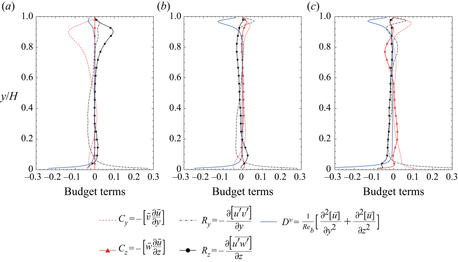
All the budget terms are normalized by the bulk mean velocity $U_b$ and duct height $H$. The budget term profiles at three different locations $z/H=0.0, 0.25$ and $0.375$ are shown in figure 12. We first focus on the profiles in the bottom half of the clear flow region ($0<y/H<0.5$). In the symmetry plane shown in figure 12(a), the 3-D effects due to the vertical convection term, $C_y$, and the horizontal Reynolds shear stress term, $R_z$, substantially contribute in the region $0.04<y/H<0.2$. This may explain the discrepancy in the turbulence intensity profiles away from the porous medium. As shown in figure 12(b,c), as expected, the 3-D effects by the convection terms ($C_y$ and $C_z$) and the horizontal Reynolds shear stress term ($R_z$) play a significant role in the momentum transport as they approach the lateral wall.

Figure 12.

Budget terms in the Reynolds-averaged streamwise momentum equation. $(a)$ Profiles in the symmetry plane at $z/H=0.0$, $(b)$ profiles at $z/H=0.25$ and $(c)$ profiles at $z/H=0.375$.

When we focus on the profiles in the top half of the clear flow region ($0.5<y/H<1.0$), it is immediately clear that the 3-D effects by the convection terms are much more prominent. In figure 12(a), in the symmetry plane, the vertical convection term, $C_y$, by the downward mean flow contributes to a significant momentum loss, which principally causes the deviation of the mean velocity profile from the established law of the wall for 2-D flows observed in figure 9(a). As the upward secondary flow is induced near the lateral wall as observed in figure 8, the vertical convection, $C_y$, causes the momentum gain at $z/H=0.25$ and $0.375$ shown in figures 12(b) and 12(c). At $z/H=0.25$ and $0.375$ in figures 12(b) and 12(c), the terms $C_y$ and $R_y$ transport the high-momentum fluid towards the top wall making the boundary layer thinner as observed in the mean velocity contour shown in figure 8(a). This results in the increase in the wall shear stress around $z/H=0.3$ as shown in figure 7(a). As opposed to the role of the upward flow, the downward flow in the symmetry plane thickens the boundary layer of the top wall, resulting in the reduction of the wall shear stress in the middle of the top wall as observed in figure 7(a).

8. Mean temperature

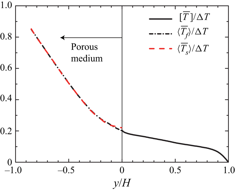
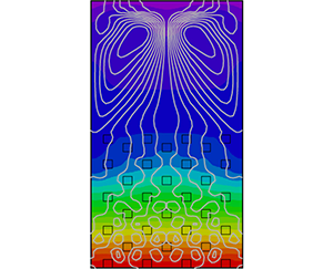
While the previous sections concentrate on the flow field properties, this section provides discussions of the mean temperature distribution. A contour map of the non-dimensional mean temperature distribution, $\bar {T}^*=\left ({[\bar{T}]} - T_{y=0}\right )/\Delta T$, is presented in figure 13(a) and the mean temperature profile at $z/H=0.0$ is plotted in figure 14, where the volume-averaged temperature profiles for fluid and solid phases are shown in the porous medium region. In addition, to better understand a global view of the heat and fluid flow, the heatlines proposed by Kimura & Bejan (Reference Kimura and Bejan1983) are superimposed in figure 13(a), and the secondary flow intensity with the cross-sectional streamlines is presented in figure 13(b). The heatlines defined in analogy with streamlines are expressed as the iso-contour lines of heat function $H_f$, and are defined as follows:

(8.1)\begin{equation} \left. \begin{aligned} \frac{\partial H_f}{\partial y} & = \rho c_p {\left[ \bar{w} \right]} \left({[\bar{T}]}-T_0\right) +\rho c_p {\left[ \overline{w'T'} \right]}- k_f \frac{\partial {[\bar{T}]}}{\partial z},\\ \frac{\partial H_f}{\partial z} & = \rho c_p {\left[ \bar{v} \right]} \left({[\bar{T}]}-T_0\right) +\rho c_p {\left[ \overline{v'T' } \right]}- k_f \frac{\partial {[\bar{T}]}}{\partial y}, \end{aligned} \right\} \end{equation}

Figure 13.

$(a)$ Contour map of the mean temperature together with the heatlines. $(b)$ Contour map of the secondary flow intensity together with the streamlines. For the streamlines, white lines correspond to clockwise rotation and black lines to anticlockwise rotation.

Figure 14.

Mean temperature profiles. The mean solid- and fluid-phase temperatures averaged over the REV, ${\langle \overline {T_f} \rangle }^{f}$ and ${\langle \overline {T_s} \rangle }^{f}$, are shown in the porous medium region $y/H<0$, while ${\left [ \overline {T_f} \right ]}$ is shown in the clear fluid region.

where $c_p$ and $T_0$ are the constant-pressure specific heat and reference temperature, respectively. The iso-lines of the heat function, which is similar to the stream function for the streamlines, can visualize the heat flow due to the combined effects of convection, turbulent transport and heat conduction. It is noted that although several choices are possible for the reference temperature $T_0$, we set the reference temperature as the mean temperature at the porous wall interface (we have confirmed that the conclusion does not change even if we change the reference temperature).

Figure 13 confirms that the heatlines in the clear flow region exhibit the large-scale recirculating patterns as in the streamlines of the secondary flow, which is characterized by the upward flow along the lateral walls and downward flow in the symmetry plane. This indicates that the secondary flow considerably alters the mean temperature fields despite the fact that the intensity of the secondary flow is not very strong (6 % of the bulk mean velocity). It is also evident that the upward flow along the lateral wall convects the high-temperature fluid towards the top wall, while the downward flow in the symmetry plane convects the near-wall low-temperature fluid towards the core region. This leads to a considerably non-uniform temperature distribution in the horizontal direction despite the fact that the temperature difference is not imposed to the lateral walls. This is reasonably reflected by the wall heat flux profile at the top wall as shown in figure 7(b) where the wall heat flux takes a maximum value at around $z/H=0.3$ and decreases as it approaches the middle of the top wall.

The other observation in figures 13(a) and 14 is that the mean temperature inside the porous medium region ($y/H<0$) varies more significantly than that in the clear flow region ($y/H>0$). Similar observations were made in the conjugate heat transfer of a turbulent porous-walled channel by Nishiyama et al. (Reference Nishiyama, Kuwata and Suga2020), where it was reported that the mean temperature deep inside the porous wall region varied significantly as the turbulent heat flux was damped, and the heat conduction was more effective in this region. Indeed, the Nusselt number representing the heat transfer in the porous medium region $Nu_p$ is nearly unity, $Nu_p=1.0$, suggesting the generally linear variation of the mean temperature deep in the porous medium region as shown in figure 14. Also, figure 14 confirms that the fluid- and solid-phase temperature profiles are observed to collapse into each other, implying that the temperature inside the porous wall region nearly reaches the equilibrium state even just below the porous interface, which is consistent with the results for the conjugate heat transfer of porous channel flow Nishiyama et al. (Reference Nishiyama, Kuwata and Suga2020). This is principally due to the relatively low conductivity ratio and low turbulent heat transfer rate in the porous medium region. It is expected that an increase in the heat conduction through the porous material leads to an increase in the solid-phase temperature while an enhancement of the turbulent heat transfer leads to a decrease in the fluid temperature, resulting in the separation between solid- and fluid-phase temperatures. The other important implication from figure 14 is that the temperature field in the present system can be predicted neither with the isothermal wall condition nor with the constant wall heat flux condition at the surface of the porous medium because the solid-phase temperature is far from homogeneous. This demonstrates the importance of employing the conjugate heat transfer approach for studying the turbulent heat transfer over porous walls. Note that although the necessity of conjugate heat transfer depends on the thermal properties and flow condition, the ratio of the thermal diffusivity between the air and the metal material is of the same order as that employed in the present simulation. It should be noted that, although the results are not shown here, we confirmed that the difference in the thermal boundary conditions of the porous material considerably affects the temperature field inside the porous medium region ($y/H<0$) while the heat transfer mechanism in the clear flow region ($y/H>0$) is consistent irrespective of the choice of the thermal boundary conditions of the porous medium. A similar observation was made in the DNS study of porous channel flow reported in Nishiyama et al. (Reference Nishiyama, Kuwata and Suga2020), which showed that, over the porous wall, profiles of the mean temperature and temperature variance were not affected by the choice of the thermal boundary conditions.

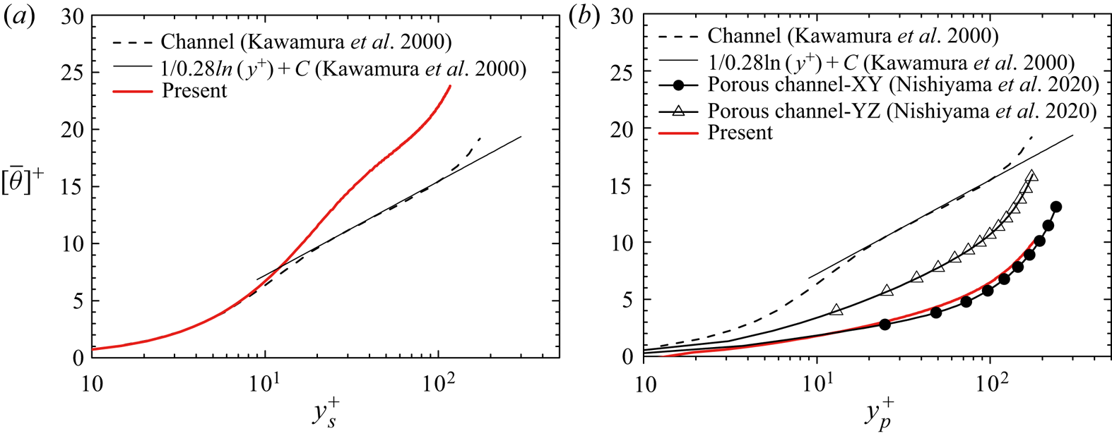
To discuss the scaling of the mean temperature profile, inner-scaled mean temperature profiles are shown as in the velocity profiles. Figure 15(a) displays a profile of the mean temperature, ${[\bar{\theta}]}={[ \bar {T}]}-T_{y=H}$, normalized by the local friction temperature at the middle of the top wall, $z/H=0.0, y/H=1.0$, with the top wall coordinate. For a comparison, the DNS result for a turbulent channel flow in constant wall temperature difference conditions at $Re_\tau =180$ and an empirical log-law profile from Kawamura, Abe & Shingai (Reference Kawamura, Abe and Shingai2000) are also presented. Although the profiles in the viscous sublayer ($y_s^+<10$) are consistent in the channel and porous duct flows, the profile for the porous duct flow considerably deviates upward when it approaches the core region. This trend is similar to that observed in the inner-scaled mean velocity profile in figure 9(a); it is related to the lateral wall effects characterized by the enhanced secondary flow motion.

Figure 15.

Inner-scaled mean temperature in log–linear format. $(a)$ Profile near the top wall and $(b)$ profile over the porous medium. DNS data of the turbulent channel flow from Kawamura et al. (Reference Kawamura, Abe and Shingai2000) and porous-walled channel flows from Nishiyama et al. (Reference Nishiyama, Kuwata and Suga2020) are included.

A profile of the mean temperature, $\left [ \bar {\theta } \right ]={[\bar{T}]}_{y=0,z=0} - {[\bar{T}]}$, over the porous medium is displayed in figure 15(b), where the friction temperature at the porous–fluid interface $y/H=0.0, z/H=0.0$ is evaluated via the total heat flux at the interface averaged over $-\ell _z/2 < z < \ell _z/2$: $({\mu }/{Pr}) ({\partial {\left [ \bar {\theta } \right ]}}/{\partial y}) - \rho c_p {[\bar {\theta } \ \bar {v}]} - \rho c_p {[\overline {\theta 'v'}]}$. Also shown are the DNS results of turbulent flows over anisotropic orthogonal media for comparable Reynolds number cases from Nishiyama et al. (Reference Nishiyama, Kuwata and Suga2020): cases YZ ($Re_\tau ^p=180$ and $Re_K=4.9$) and XY ($Re_\tau ^p=240$ and $Re_K=6.0$). Note that the displacement $d_p^+$ is not taken into account for the distance from the porous wall because the logarithmic region of the temperature profile cannot be observed even though $d_p^+$ is introduced. Although the narrow logarithmic region can be confirmed in the profile of the smooth-wall channel according to Kawamura et al. (Reference Kawamura, Abe and Shingai2000), the logarithmic region is no longer preserved for the porous channel and porous duct flow results. Moreover, the profiles over the porous media deviate downward owing to the increase in the heat transfer over the porous media. Interestingly, the profile of the porous duct flow is in good agreement with the porous channel flow in case XY, suggesting that the mean temperature profile is not significantly affected by the lateral walls as in the mean velocity profiles.

9. Turbulent heat flux

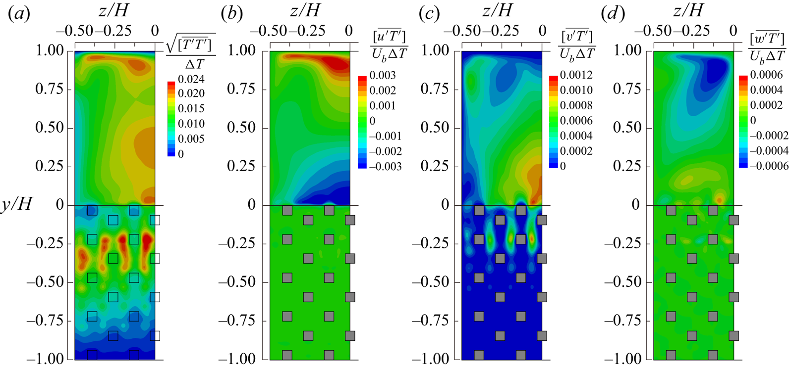
Before discussing the heat transfer mechanisms by analysing the energy budget terms, this section discusses the effects of the lateral walls on the turbulent heat flux distributions. The turbulent heat flux components and mean square temperature variance are shown in figure 16. The temperature variance shown in figure 16(a) near the symmetry plane exhibits two prominent peaks: one is located above the porous–fluid interface and the other is located inside the porous medium at around $y/H=-0.25$. Interestingly, the temperature variance is enhanced considerably in the porous medium region rather than over the porous medium, despite the fact that turbulent velocity fluctuations are increased over the porous medium. This trend is consistent with the results for the conjugate heat transfer in porous-walled channel flow of Nishiyama et al. (Reference Nishiyama, Kuwata and Suga2020). They analysed the production terms in the transport equation of the temperature variance and concluded that the local maximum peak over the porous medium was due to the increased vertical velocity fluctuations, whereas inside the porous medium it was due to the increased temperature gradient, both of which contributed to the production of the temperature variance. The streamwise turbulent heat flux in figure 16(b) is slightly enhanced over the porous wall and rapidly damped in the porous medium region as in the streamwise Reynolds stress shown in figure 10(a). The reason is that the Reynolds shear stress component, which dominantly contributes to the generation of the streamwise turbulent heat flux, is rapidly decayed as well (not shown here). In contrast to the streamwise component, figure 16(c) shows that the vertical turbulent heat flux near the symmetry plane exhibits two prominent peaks that are located above and inside the porous medium. This trend is similar to that seen for the temperature variance. Indeed, both production terms for the temperature variance and vertical turbulent heat flux are related to the vertical mean temperature gradient and vertical velocity fluctuations. The presence of the lateral heat flux, which vanishes in 2-D flow systems as in turbulent channel flow, can be confirmed in figure 16(d). Although the magnitude is much smaller than those of the vertical and streamwise components, the lateral turbulent heat flux is particularly generated near the top wall where the gradient of the horizontal mean velocity that contributes to the generation term is significantly increased. As in the turbulence intensities, it is apparent that the contours of the turbulence heat flux and temperature variance are not flattened near the symmetry plane affected by the lateral walls.

Figure 16.

$(a)$ Temperature variance, $(b)$ streamwise turbulent heat flux, $(c)$ vertical turbulent heat flux and $(d)$ lateral turbulent heat flux.

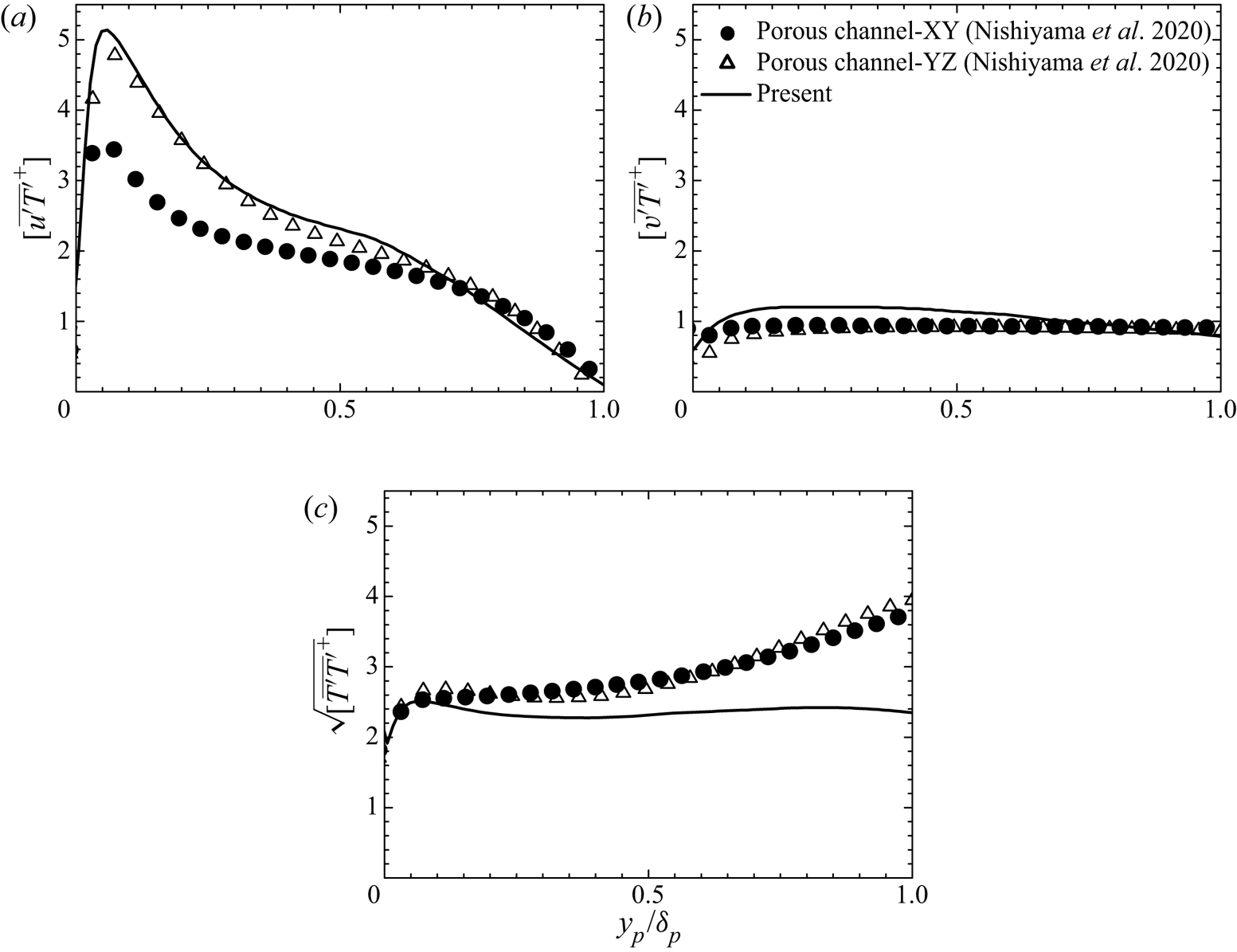
The influence of the lateral wall effects on the temperature variance can be clearly observed in figure 17, which presents comparisons of turbulence statistics related to the temperature variance with those for the porous channel flows at comparable Reynolds numbers from Nishiyama et al. (Reference Nishiyama, Kuwata and Suga2020). Although figure 15(b) shows that the mean temperature profile for the present result is close to that in case XY, the streamwise turbulent heat flux in figure 17(a) for the porous duct is considerably larger than that in case XY but close to that in case YZ. Moreover, figures 17(b) and 17(c) confirm that the profiles of the vertical turbulent heat flux and temperature variance for the porous duct flow distinctly deviate from the results for the channel flows. In contrast with the results for the channel flows, the vertical component in figure 17(b) is larger just above the porous medium but slightly smaller near the core of the duct, and the temperature variance in figure 17(c) is considerably smaller near the core of the duct.

Figure 17.

$(a)$ Streamwise turbulent heat flux, $(b)$ vertical turbulent heat flux and $(c)$ temperature variance. The DNS data of porous-walled channel flows from Nishiyama et al. (Reference Nishiyama, Kuwata and Suga2020) are included.

These observations in figures 15 and 17 suggest that, over the porous medium region, the presence of the lateral walls does not significantly affect the scaling of the first moment (i.e. mean temperature and mean velocity) in the symmetry plane, but the apparent effects emerge in the second moments such as the turbulence intensity, temperature variance and turbulent heat flux. By contrast, near the top wall, the effects of the lateral walls are more prominent than the square duct flow, even modifying the scaling of the first moment in the symmetry plane. Further discussion about the influence of the lateral wall can be addressed by studying the effects of the aspect ratio as in Vinuesa et al. (Reference Vinuesa, Noorani, Lozano-Durán, Khoury, Schlatter, Fischer and Nagib2014).

10. Heat transfer mechanisms

The previous sections gave a brief review of the temperature fields. This section finally reveals the detailed heat transfer mechanisms by analysing budget terms in the energy equation. In the clear flow region, the Reynolds-averaged energy equation for the present flow system may be written as follows:

(10.1)\begin{equation} {\left[ \bar{v}\frac{\partial \bar{T}}{\partial y } \right]} + {\left[ \bar{w}\frac{\partial \bar{T}}{\partial z} \right]} = -\frac{\partial {\left[ \overline{v'T'} \right]}}{\partial y } -\frac{\partial {\left[ \overline{w'T'} \right]}}{\partial z } +\frac{1}{PrRe_b}\left(\frac{\partial^2 {[\bar{T}]}}{\partial y^2 }+\frac{\partial^2 {[\bar{T}]}}{\partial z^2 } \right), \end{equation}

where the equation is non-dimensionalized by the bulk mean velocity $U_b$, duct height $H$ and temperature difference $\Delta T$. The terms $C^T_y=- {\left [ \bar {v}\left ({\partial \bar {T}}/{\partial y }\right ) \right ]}$ and $C^T_z=- {\left [ \bar {w}\left ({\partial \bar {T}}/{\partial z}\right ) \right ]}$ denote the vertical and horizontal convection terms, respectively. The turbulent transport terms are $H_y=-({\partial {\left [ \overline {v'T'} \right ]}}/{\partial y })$ and $H_z= -\left ({\partial {\left [ \overline {w'T'} \right ]}}/{\partial z }\right )$. The last term on the right-hand side is the conduction term $D^{\nu T}=1/(Pr Re_b)\left ({\partial ^2 {[\bar{T}]}}/{\partial y^2 }+{\partial ^2 {[\bar{T}]}}/{\partial z^2 }\right )$.

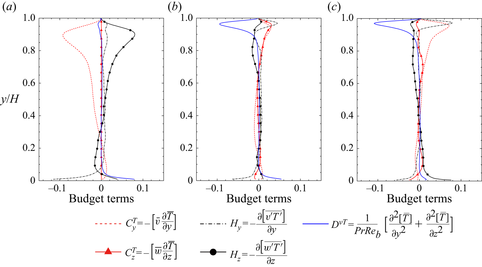
The budget term profiles at different locations $z/H=0.0, 0.25$ and $0.375$ are presented in figure 18. First, we focus on the profiles in the top half of the clear flow region. In the symmetry plane as shown in figure 18(a), the vertical convection $C^T_y$ works as an energy loss in the region $0.3<y/H<1.0$ where the horizontal turbulent transport $H_z$ is almost balanced by $C^T_y$. The negative vertical convection in this region $(0.3<y/H<1.0)$ indicates that the downward secondary flow in the symmetry plane convects the near-wall low-temperature fluid towards the core region, supporting the view made in the mean temperature contour with the heatlines in figure 13(a). Moreover, this convection process thickens the thermal boundary layer in the middle of the top wall, which causes a reduction of the viscous term and wall heat flux as observed in figure 7(b). Near the lateral wall at $z/H=0.375$ in figure 18(c), both $H_y$ and $C^T_y$ work as an energy source and convect the high-temperature fluid towards the top wall, resulting in significantly increased $D^{\nu T}$. The heat transfer mechanisms near the top wall are similar to the momentum transport. The upward secondary flow along the lateral wall convects the high-momentum fluid towards the top wall, while the downward flow in the symmetry plane convects the near-wall low-momentum fluid towards the core region, thus leading to the similarity between the wall heat flux and wall shear stress distributions at the top wall. Near the corners above the porous medium, the heat transfer mechanisms are much more complex than the momentum transport, and the 3-D effects are more notable. For the momentum transport near the corners above the porous medium shown in figure 12(c), the vertical turbulent transport term tends to be balanced by the viscous term, and the contributions of the convection terms due to the secondary flow $C_z$ and $C_y$ are less than 30 % of $R_y$. In contrast, for the heat transfer in the vicinity of the porous medium wall ($0<y/H<0.05$) as shown in figure 18(c), the horizontal turbulence transport term $H_z$ is the most dominant contributor and causes an energy gain, while $H_y$ and $C^T_z$ work as an energy loss. The contribution of the convection by the horizontal secondary flow $C^T_z$ is found to be 45 % of $H_y$, suggesting that the secondary flow largely affects the temperature fields in this region.

Figure 18.

Budget terms of the Reynolds-averaged energy equation. $(a)$ Profiles in the symmetry plane at $z/H=0.0$, $(b)$ profiles at $z/H=0.25$ and $(c)$ profiles at $z/H=0.375$.

To better understand the heat transfer mechanism inside the porous medium, we consider the volume- and Reynolds (double)-averaged energy equations. The analysis of the double-averaged equation is not only helpful for discussing heat transfer mechanisms from a macroscopic viewpoint, but also provides indispensable data for the progression of macroscopic turbulence models. Applying the volume- and Reynolds-averaging operators to the energy equation for the fluid phase, we can obtain the double-averaged energy equation for the fluid phase, normalized by $U_b$, $H$ and $\Delta T$, as follows:

(10.2)\begin{align} \underbrace{\varphi {\langle \overline{u_j} \rangle} \frac{\partial {\langle \overline{T_f} \rangle} }{\partial x_{j}}}_{-C^{T}_p} &= \underbrace{\frac{1}{Pr\,Re_b}\frac{\partial}{\partial x_{j}}\left( \frac{\partial \varphi {\langle \overline{T_f} \rangle}}{\partial x_{j}} +\frac{1}{\Delta V}\int_A n_j \overline{T_f}\,\textrm{d}A \right) }_{D^{\nu T}_p } \nonumber\\ &\quad \underbrace{-\frac{\partial}{\partial x_{j}} \varphi {\langle \overline{u_j' T_f} \rangle}}_{H_p} \underbrace{-\frac{\partial}{\partial x_{j}} \varphi {\langle \tilde{\bar{u}}_j \widetilde{\overline{T_f}} \rangle} }_{\mathcal{H}_p} \underbrace{+\frac{1}{Pr\,Re_b \Delta V}\int_A n_j \frac{\partial \overline{T_f}}{\partial x_{j}}\,\textrm{d}A}_{S_w}, \end{align}

where $T_f$ is the fluid-phase temperature and the terms $C^{T}_p$, $D^{\nu T}_p$, $H_p$, $\mathcal {H}_p$ and $S_w$ are the convection, diffusive heat flux, turbulent heat flux, dispersion heat flux and wall heat transfer terms, respectively. The diffusive heat flux term consists of the molecular diffusion term and the surface integrating term referred to as the tortuosity molecular diffusion term (Kuwahara, Nakayama & Koyama Reference Kuwahara, Nakayama and Koyama1996; Nakayama & Kuwahara Reference Nakayama and Kuwahara1999). See Saito & de Lemos (Reference Saito and de Lemos2005) for the detailed derivation of the volume-averaged energy equation. The convection term $C^{T}_p$ represents the transport process owing to the volume-averaged mean flow ${\langle \overline {u_i} \rangle }$, i.e. the convection term by the global mean flow current. The dispersion heat flux term $\mathcal {H}_p$ represents the transport process by the mean velocity dispersion which is the deviation from the macroscopic mean velocity, $\tilde {\bar {u}}_i = \overline {u_i} - {\langle \overline {u_i} \rangle }$. The surface integration terms in $D^{\nu T}_p$ and $S_w$ arise because the averaging of the gradient provides an additional integration term as given by Whitaker (Reference Whitaker1996):

(10.3)\begin{equation} \varphi {\left\langle \frac{\partial \phi}{\partial x_j} \right\rangle} = \frac{\partial \varphi {\langle \phi \rangle}}{\partial x_j} + \frac{1}{\Delta V} \int_A n_j \phi\,\textrm{d}A, \end{equation}

where $\Delta V=\ell _x \ell _y \ell _x$ is the volume of the REV as illustrated in figure 2. The surface of the porous medium is $A$ and $n_j$ is a unit normal vector pointing outward from the fluid to the solid phase.

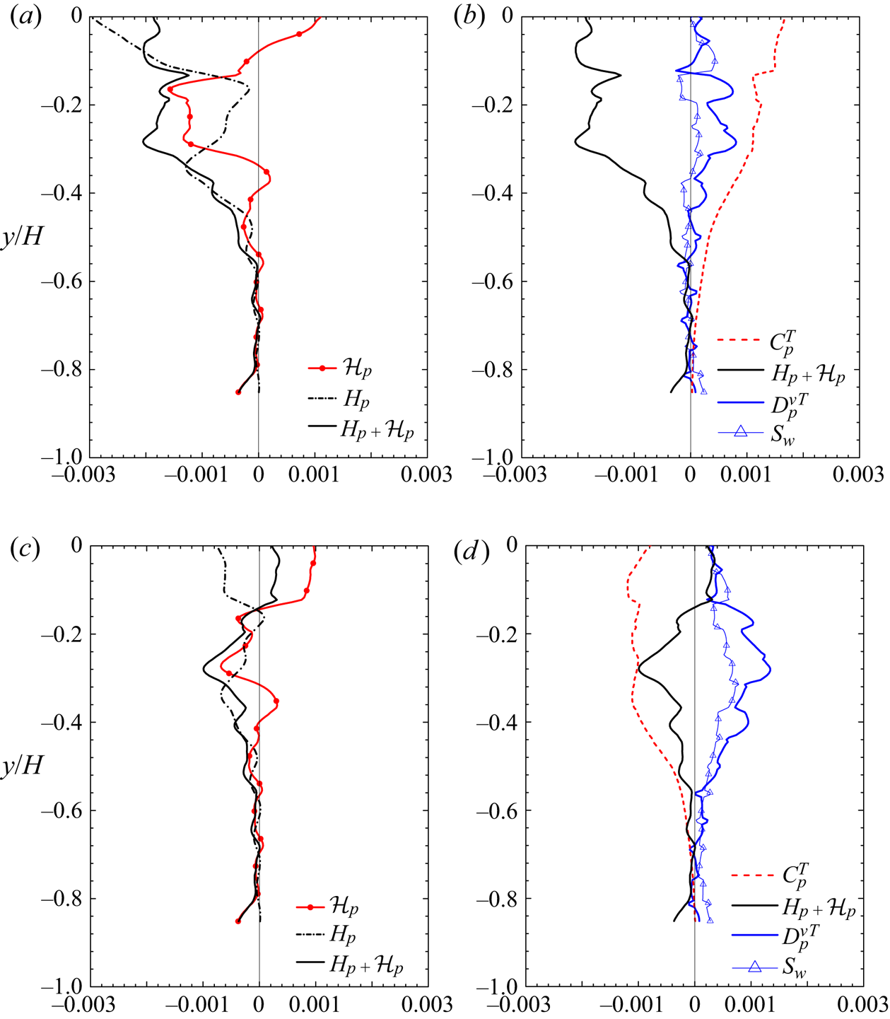
The budget term profiles along the vertical direction are computed by continuously shifting the REV from $y=-H+\ell_y/2$ to $y=0$. The profiles of these budget terms in the symmetry plane $(z/H = 0.0)$ and those near the lateral wall ($z/H=0.35$) are plotted in figure 19. Figure 19(a) shows that the profile of the turbulent heat flux term, $H_p$, is not monotonic inside the porous medium region: the profiles of $H_p$ exhibit a negative local minimum value around $y/H=-0.18$ while its magnitude increases towards the porous–fluid interface. This is associated with the double peaks of the vertical turbulent heat flux in figure 16(c) around $y/H=-0.25$ and $y/H=0.1$ near the symmetry plane. What is particularly interesting is that the trends of the dispersion heat flux term $\mathcal {H}_p$ and $H_p$ are opposite. It is observed from figure 19(a) that $\mathcal {H}_p$ increases where the region $H_p$ decreases. This trend can be explained from the transport equations of $\mathcal {H}_p$ and $H_p$, wherein one of the production terms appears in the same form but with opposite sign (Suga et al. Reference Suga, Chikasue and Kuwata2017). Suga et al. (Reference Suga, Chikasue and Kuwata2017) suggested in their large-eddy simulation study of the turbulent heat transfer inside porous media that since the transport equations of $\mathcal {H}_p$ and $H_p$ included the mutual energy exchange terms, the sum of those fluxes can be modelled more easily than treating the individual terms. Accordingly, a profile of $H_p+\mathcal {H}_p$ is presented in figure 19(a), and this reveals that the total heat flux term ($H_p+\mathcal {H}_p$) in the symmetry plane works as an energy loss. Figure 19(b) confirms that this energy loss is found be almost balanced by the energy gain due to the convection term $C^T_p$, as a result of the global flow mean flow current, which is induced by the secondary flow penetration towards the porous medium region. The corner flow above the porous medium wall at $y/H=0.0, z/H=\pm 0.5$ partly penetrates the porous medium wall, and this flow ejects the fluid in the porous wall near the symmetry plane towards the clear flow region. Then, as observed in figure 13(b), recirculating mean flow patterns across the porous–fluid interface are generated, thus enhancing heat transfer below the porous wall. It is notable that although this recirculating mean flow is relatively weak deep inside the porous medium, the influence of this global flow on the heat transfer is still dominant deep inside the porous wall region at $y/H=-0.6$.

Figure 19.

Budget terms of the volume- and Reynolds-averaged energy equation for the fluid phase. $(a)$ Profiles of $H_p$ and $\mathcal {H}_p$ at $z/H=0.0$, $(b)$ budget terms at $z/H=0.0$, $(c)$$H_p$ and $\mathcal {H}_p$ profiles at $z/H=0.35$ and $(d)$ budget terms at $z/H=0.35$.

Although figure 19(b) confirms that the total heat flux term $(H_p+\mathcal {H}_p)$ largely contributes the heat transfer in the symmetry plane, figure 19(c) shows that the total heat flux term is significantly reduced due to the lateral wall; still, $H_p$ and $\mathcal {H}_p$ have opposite trends as in figure 19(a). Figure 19(d) confirms that $C^T_p$ works as an energy loss, indicating that the global mean flow induced by the secondary flow penetration convects the low-temperature flow in the clear flow region towards the porous medium region. The lateral wall reduces the contribution of the turbulent heat flux while the molecular diffusive term $D^{\nu T}_p$ and the wall heat transfer term $S_w$ become more prominent. The wall heat transfer, which transports the energy by heat conduction through the solid phase, convects the high-temperature fluid as in $D^{\nu T}_p$. The magnitude of $S_w$ is smaller than that of $D^{\nu T}_p$ despite that the thermal diffusivity is 4.4 times larger, which is due to the relatively high porosity of the porous medium under consideration. The solid phase merely occupies 23 % of the REV. The observation that the contribution of $S_w$ is substantial and non-uniform confirms the importance of employing conjugate heat transfer conditions because the non-uniform contribution of $S_w$ cannot be reproduced except for conjugate heat transfer conditions.

The other important finding in this analysis is that the dispersion heat flux plays an important role in the heat transfer, which is not reproduced by simulations based on the VANS equations in prior studies (Breugem et al. Reference Breugem, Boersma and Uittenbogaard2006; Samanta et al. Reference Samanta, Vinuesa, Lashgari, Schlatter and Brandt2015). This finding also suggests that the VANS approach essentially needs some model that considers the dispersion effects to correctly predict the heat transfer in the porous medium region.

Finally, it should be noted that the turbulent heat transfer of a porous square duct flow largely depends on the characteristics of the porous material. In this study, we consider highly permeable porous materials, which can be encountered in the carbon paper of fuel cells, foam metal in heat exchangers or catalytic converters. However, for porous media with lower permeability or void fraction, such as packed beds, the turbulence enhancement over the porous wall is expected to be less significant (Breugem et al. Reference Breugem, Boersma and Uittenbogaard2006; Suga et al. Reference Suga, Matsumura, Ashitaka, Tominaga and Kaneda2010; Rosti, Cortelezzi & Quadrio Reference Rosti, Cortelezzi and Quadrio2015; Kuwata & Suga Reference Kuwata and Suga2019). This weakens the secondary mean flow leading to a decrease in convective heat transfer by the secondary mean flow. In addition, since flow penetration towards the porous media is weakened, the convective heat transfer inside the porous media is also reduced. Therefore, high heat transfer performance due to enhanced secondary flow is not expected to be achieved by porous media with low permeability.