1. Introduction
Flow through annular sections, whether concentric or eccentric, is a fundamental phenomenon present in various industrial applications and research fields. Early studies of eccentric annuli were motivated by the misalignment that often occurs in originally concentric configurations, particularly in heat exchangers (Snyder & Goldstein Reference Snyder and Goldstein1965). Various factors, including high internal pressures and the presence of spacer pads, among others, can cause such deviations of the single concentric annular tube. This topic continues to attract attention in modern engineering applications, especially in nuclear power plants, where deviations from concentricity significantly affect heat transfer in pressurised heavy water reactors and heat exchangers (Pothukuchi et al. Reference Pothukuchi, Kelm, Patnaik, Prasad and Allelein2018). Another important engineering application arises in the petroleum industry, where this type of geometry is encountered in processes such as drilling and cementing, which are critical to oil extraction. While concentric configurations can approximate these physical issues, eccentric annuli may more accurately reflect real operating conditions (Haciislamoglu & Langlinais Reference Haciislamoglu and Langlinais1990; Lou & Peden Reference Lou and Peden1990).
Additionally, the motivation for this work stems from the study of biological fluids that, under certain circumstances, can be present in annular geometries, as described below. Understanding the flow and dispersion of solutes using biofluids is essential for managing the distribution of drugs, nutrients and metabolic waste (Kelley & Thomas Reference Kelley and Thomas2023). Specifically, the circulation mechanism of cerebrospinal fluid is linked to various neurological disorders and conditions, including Alzheimer’s disease, multiple sclerosis, hydrocephalus and syringomyelia (Sánchez et al. Reference Sánchez, Martínez-Bazán, Gutiérrez-Montes, Criado-Hidalgo, Pawlak, Bradley, Haughton and Lasheras2018; Deisenhammer et al. Reference Deisenhammer, Zetterberg, Fitzner and Zettl2019). Annular configurations can effectively simulate drug delivery through the spinal cord, facilitated by the flow of cerebrospinal fluid. These geometries can also be achieved through catheterisation, a medical procedure utilised for both diagnostic and treatment purposes. This technique is commonly employed in the management of cardiovascular, urological, ophthalmic, neurovascular and gastrointestinal conditions (Alsemiry, Sayed & Amin Reference Alsemiry, Sayed and Amin2022). Many biological and industrial fluids, including blood and cement slurries, exhibit non-Newtonian characteristics that can be effectively captured using viscoelastic models (Yin & Zhu Reference Yin and Zhu2006). Linear constitutive equations such as those of Maxwell, Jeffreys and generalised Maxwell (Bird, Stewai & Lightfoot Reference Bird, Stewai and Lightfoot2002) are appropriate for small deformation gradients and have been successfully applied to describe biological fluids (Yin & Zhu Reference Yin and Zhu2006; Raikher, Rusakov & Perzynski Reference Raikher, Rusakov and Perzynski2013; Yang et al. Reference Yang, Christov, Griffiths and Ramon2020).
When the deformation gradients become larger, nonlinear viscoelastic models are typically required. Examples include the Oldroyd-B model (Yeleswarapu et al. Reference Yeleswarapu, Kameneva, Rajagopal and Antaki1998; Sajid et al. Reference Sajid, Zaman, Ali and Siddiqui2015) and the Giesekus model, which has been successfully used to describe polymeric fluids (Wang et al. Reference Wang, Wang and Liu2022, Reference Wang, Ni, Wang and Liu2023). In the present study, we focus on the regime of small deformation gradients; therefore, the linear Maxwell model is employed.
Resolving boundary value problems in configurations with eccentricity presents unique challenges due to the inherent asymmetry, which complicates the definition of boundary conditions (Chen, Tsai & Liu Reference Chen, Tsai and Liu2009). Various approximation methods have been proposed in the literature, particularly in cylindrical coordinates; however, these methods are primarily effective only in the limiting case of small eccentricities, such as the domain perturbation method (Aziz & Na Reference Aziz and Na1984; Leal Reference Leal2007). In their research, El-Saden (Reference El-Saden1961) developed a general analytical solution to Poisson’s equation by utilising a bipolar coordinate transformation to study heat conduction in an eccentric hollow cylinder. Building on this work, Snyder & Goldstein (Reference Snyder and Goldstein1965) applied the relevant boundary conditions and derived an analytical expression for the velocity profile applicable for any degree of eccentricity. Their findings demonstrate that the velocity profile increases with increasing eccentricity.
The dispersion of solutes by the flow within a channel results in a combined advective-diffusive transport process. In his classic work, G. I. Taylor (Reference Taylor1953) approached this problem heuristically by considering the cross-sectional average concentration. He demonstrated that, at long times, the mean concentration disperses through what appears to be pure diffusion. The resulting virtual diffusion coefficient, now commonly referred to as the effective dispersion coefficient, encapsulates the combined effects of convective and diffusive transport (Taylor Reference Taylor1953). Building on Taylor’s work, Aris (Reference Aris1956) employed the method of moments to generalise this theory, deriving a comprehensive expression for advection-diffusion transport concerning the mean concentration. For solute dispersion in eccentric annular spaces, Sankarasubramanian & Gill (Reference Sankarasubramanian and Gill1971) applied bipolar coordinate transformations along with the Aris–Taylor theory (Aris Reference Aris1956). They proposed an exact solution based on series expansions that were intended to be valid for all time values. However, due to the complexity of the resulting equations, their analysis was limited to deriving asymptotic values of the effective coefficients for long times. Later, Chu et al. (Reference Chu, Garoff, Tilton and Khair2020) demonstrated that this analysis is only applicable for small eccentricities and extended it to include both steady and time-oscillatory flows. Their semi-analytical formulation enabled the calculation of effective dispersion coefficients across the full range of eccentricities, except the singular point where the eccentricity equals zero,
 $\phi = 0$
, at which the bipolar coordinate system becomes undefined. In line with the findings of Sankarasubramanian & Gill (Reference Sankarasubramanian and Gill1971), Chu et al. (Reference Chu, Garoff, Tilton and Khair2020) concluded that the effective dispersion coefficient increases as eccentricity rises. They also observed that this coefficient can be further enhanced in the case of slow oscillation.
Building on our earlier discussion, we apply a bipolar coordinate transformation to the governing equations that need to be solved. Furthermore, we employ homogenization theory (Mei & Vernescu Reference Mei and Vernescu2010; Muñoz et al. Reference Muñoz, Arcos, Bautista and Méndez2018; Chu et al. Reference Chu, Garoff, Tilton and Khair2020) to derive the effective dispersion coefficient for the pulsatile flow of viscoelastic fluids through an eccentric annular tube.
This paper is composed of the following sections. In § 2, we present the governing equations of the physical problem. Both the momentum and mass transport equations are transformed into a bipolar coordinate system and represented in dimensionless form. In § 3, considering the linearity of the resulting momentum equation, we have decomposed it into its steady and oscillatory parts to apply the homogenization method correctly. The time-independent equations for steady and oscillatory components are solved numerically. In § 4, we identify the different time scales involved in the physical problem. Based on the difference in spatial scales, a small parameter is defined that enables the application of multiple-scale analysis in conjunction with the homogenization method. Finally, in § 5, the numerical results are validated and discussed to evidence the effects of viscoelasticity on the effective dispersion coefficient and the mean concentration.
2. Problem formulation and governing equations
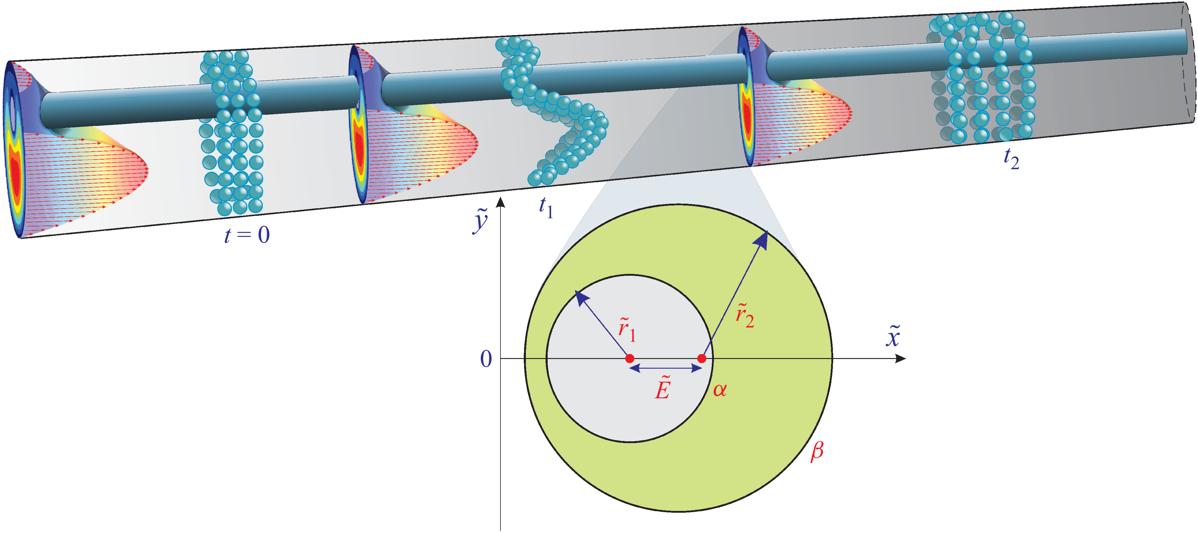
We examine the dispersion of a neutral solute within an eccentric annular tube (figure 1) in a pulsating flow of a viscoelastic fluid. The inner and the outer cylinders of the eccentric annular tube have radii
 $\tilde {r}_1$
and
 $\tilde {r}_2$
, respectively, and
 $\tilde {\ell }$
is the length of the tube. The offset between the centres of the cylinders is denoted by
 $\tilde {E}$
. For analysing this problem, we assume the following: (a) incompressible fluid with constant physical properties, (b) laminar flow, (c) the analysis is focused far from the ends of the tube and (d) fully developed flow. The pulsatile fluid flow is caused by a time-dependent pressure gradient given by
 \begin{equation} -\frac {\partial \tilde {P}}{\partial \tilde {z}} = \tilde {G} = \tilde {G}_{0}\left [1 + g {\textrm{Re}} \left \{e^{-i\tilde {\omega } \tilde {t}} \right \}\right ], \end{equation}
where
 $\tilde {G}_{0}$
represents the pressure gradient of the steady-state part and
 $g$
is the relative amplitude of the oscillatory component relative to the steady pressure. Also,
 ${\textrm{Re}}\bigl \{\boldsymbol{\cdot }\bigr \}$
denotes the real part of the term within the brackets, while
 $i=\sqrt {-1}$
represents the imaginary unit,
 $\tilde {t}$
is the time and
 $\tilde {\omega }$
is the angular frequency.
Considering the assumptions mentioned earlier, the momentum equation is the following (Bird et al. Reference Bird, Stewai and Lightfoot2002):
 \begin{equation} \tilde {\rho } \frac {\partial \boldsymbol{\tilde {V}} }{\partial \tilde {t}} = - {\boldsymbol{\nabla }} \tilde {P} + {\boldsymbol{\nabla }}\boldsymbol{\cdot }{\tilde {\boldsymbol{\tau }}}, \end{equation}
The geometry of the eccentric annulus is described as follows:
 $\tilde {E}$
represents the offset between the centres of the circumferences and
 $\tilde {r}_{1}$
and
 $\tilde {r}_{2}$
denote the inner and outer radii, respectively. The coordinate
 $\tilde z$
is the axial direction (into/out of paper in this figure). Since bipolar coordinates will be used to solve the mathematical problem, we define
 $\alpha$
and
 $\beta$
as representing the inner and outer circles in bipolar coordinates, respectively (see (2.14)–(2.16) for the definitions of bipolar coordinates).

where
 $\tilde {\rho }$
is the fluid density and
 $\boldsymbol{\tilde {V}} =(\tilde {u}, \tilde {v}, \tilde {w})$
is the velocity vector with
 $\tilde {u}, \tilde {v}, \tilde {w}$
representing the velocity components in the directions
 $\tilde {x}$
,
 $\tilde {y}$
and
 $\tilde {z}$
, respectively. Also,
 ${\boldsymbol{\nabla }}$
is the nabla operator,
 $\tilde {P}$
is the pressure and
 $ {\tilde {\boldsymbol{\tau }}}$
is the polymeric stress tensor. The rheological behaviour of the fluid follows the linear Maxwell model given by (Tanner Reference Tanner2000)
 \begin{equation} \boldsymbol{\tilde {\tau }} + \tilde {\lambda } \frac {\partial \boldsymbol{\tilde {\tau }}}{\partial \tilde {t}} = \tilde {\mu }\left [\left (\boldsymbol{\nabla \tilde {v}} \right )^{T} + \boldsymbol{\nabla \tilde {v}}\right ]\!. \end{equation}
In this context,
 $\tilde {\lambda }$
stands for the longest relaxation time of the polymers (Bird, Armstrong & Hassager Reference Bird, Armstrong and Hassager1987; Boyko & Christov Reference Boyko and Christov2023) and
 $\tilde {\mu }$
is the polymer contribution to the shear viscosity at zero shear rate. The superscript
 $T$
indicates the transpose operator. Here, we assume that the viscous stress contribution of the Newtonian solvent can be neglected.
For this fully developed flow, we have
 $(\partial \tilde {w}/\partial \tilde {z}) = 0$
, and
 $\boldsymbol{\tilde {V}} = (0, 0, \tilde {w})$
, and therefore, (2.2) is simplified to the following equation:
 \begin{equation} \tilde {\rho } \frac {\partial \tilde {w}}{\partial \tilde {t}} = - \frac {\partial \tilde {P}}{\partial \tilde {z}} + \left [ \frac {\partial \tilde {\tau }_{xz}}{\partial \tilde {x}} + \frac {\partial \tilde {\tau }_{yz}}{\partial \tilde {y}} \right ]\!. \end{equation}
The boundary conditions for hydrodynamics are the no-slip condition,
 $\tilde {w} = 0$
, at the inner and outer surfaces. For this problem, we will solve (2.4) in the quasi-steady-state condition; that is, when the transient stage has died out, and therefore, we do not consider the initial condition for the momentum equation. Here,
 $\tilde {\tau }_{xz}$
and
 $\tilde {\tau }_{yz}$
denote the shear stress components in the planes
 $xz$
and
 $yz$
, respectively. The components of the stress tensor, from (2.3), are the following:
 \begin{align} \left (1 + \tilde {\lambda }\frac {\partial }{\partial \tilde {t}} \right )\tilde {\tau }_{xx} &= 0,\\[-11pt]\nonumber \end{align}
 \begin{align} \left (1 + \tilde {\lambda }\frac {\partial }{\partial \tilde {t}} \right )\tilde {\tau }_{yy} &= 0,\\[-11pt]\nonumber \end{align}
 \begin{align} \left (1 + \tilde {\lambda }\frac {\partial }{\partial \tilde {t}} \right )\tilde {\tau }_{zz} &= 2\tilde {\lambda }\left (\tilde {\tau }_{zx}\frac {\partial \tilde {w}}{\partial \tilde {x}} + \tilde {\tau }_{xy}\frac {\partial \tilde {w}}{\partial \tilde {y}} \right )\!,\\[-11pt]\nonumber\end{align}
 \begin{align} \left (1 + \tilde {\lambda }\frac {\partial }{\partial \tilde {t}} \right )\tilde {\tau }_{xy} &= 0,\\[-11pt]\nonumber\end{align}
 \begin{align} \left (1 + \tilde {\lambda }\frac {\partial }{\partial \tilde {t}} \right )\tilde {\tau }_{xz} &= \tilde {\mu } \frac {\partial \tilde {w}}{\partial \tilde {x}},\\[-11pt]\nonumber\end{align}
 \begin{align} \left (1 + \tilde {\lambda }\frac {\partial }{\partial \tilde {t}} \right )\tilde {\tau }_{yz} &= \tilde {\mu } \frac {\partial \tilde {w}}{\partial \tilde {y}} .\\[-11pt]\nonumber\end{align}
By appropriately combining the momentum (2.4) with the components of the stress tensor (2.9) and (2.10), the momentum equation in terms of the velocity
 $\tilde {w}$
alone is derived
 \begin{equation} \tilde {\rho } \left ( \tilde {\lambda } \frac {\partial ^2 \tilde {w}}{\partial \tilde {t}^2} + \frac {\partial \tilde {w}}{\partial \tilde {t}}\right ) = \tilde {\mu }\left ( \frac {\partial ^2 \tilde {w}}{\partial \tilde {x}^2} +\frac {\partial ^2 \tilde {w}}{\partial \tilde {y}^2} \right ) + \left ( 1 + \tilde {\lambda }\frac {\partial }{\partial \tilde {t}}\right )\left (-\frac {\partial \tilde {P}}{\partial \tilde {z}} \right )\!. \end{equation}
In the previous equation, the pressure gradient is dictated by the relationship defined in (2.1). To determine the concentration field
 $\tilde {C}(\tilde {x},\tilde {y},\tilde {z},\tilde {t})$
(mass of species per bulk volume) of the solute transported through the annular tube, the convection-diffusion equation is used
 \begin{equation} \frac {\partial \tilde {C}}{\partial \tilde {t}} + \tilde {w} \frac {\partial \tilde {C}}{\partial \tilde {z}}= \tilde {D}\left (\frac {\partial ^2 \tilde {C}}{\partial \tilde {x}^2} + \frac {\partial ^2 \tilde {C}}{\partial \tilde {y}^2} + \frac {\partial ^2 \tilde {C}}{\partial \tilde {z}^2} \right )\!, \end{equation}
where
 $\tilde {D}$
is the molecular diffusion coefficient.
The boundary conditions of (2.12) include the impermeability across the inner and outer surfaces of the annular tube, ensuring that no species penetrates through these boundaries. In addition, a symmetry condition is applied in the mid-plane
 $\tilde {y}$
. Concerning the initial condition, following the work of Chu et al. (Reference Chu, Garoff, Tilton and Khair2020), a known function is prescribed for the concentration pulse at a given axial location
 $\tilde {z}$
, and the boundary conditions for the
 $\tilde {z}$
-axis are imposed as
 $\tilde {C} = 0$
at
 $\tilde {z} = 0, \tilde {\ell }$
.
Equations (2.11) and (2.12) are utilised in the physical domain characterised by the eccentric annular geometry depicted in figure 1. Obtaining an analytical solution for boundary value problems in this geometry presents a significant challenge, as it cannot be effectively approached using Cartesian or polar coordinates (Chen et al. Reference Chen, Tsai and Liu2009). Additionally, the finite-difference method for numerical solutions cannot be directly applied to this geometry (Akyildiz, AlSohaim & Kaplan Reference Akyildiz, AlSohaim and Kaplan2019). In this work, we have transformed the Cartesian coordinates into a bipolar coordinate system, defined as outlined in Spiegel & Liu (Reference Spiegel and Liu1999) and Chu et al. (Reference Chu, Garoff, Tilton and Khair2020)
 \begin{equation} \tilde x + i \tilde y = i \tilde a \cot \left (\frac {\xi + i\eta }{2} \right )\!, \end{equation}
from which the following relationships are derived:
 \begin{align}&\qquad\quad \tilde {x} = \frac {\tilde {a} \sinh \eta }{\cosh \eta - \cos \xi }, \quad \tilde {y} = \frac {\tilde {a} \sin \xi }{\cosh \eta - \cos \xi }, \end{align}
 \begin{align}& \tilde y^2 + (\tilde x - \tilde a \textrm{coth} \eta )^2 = \frac {\tilde a^2}{\sinh ^2\eta }, \quad \tan \xi = \frac {2 \tilde y \tilde a}{\tilde x^2 + \tilde y^2 - \tilde a^2}, \end{align}
 \begin{align}&\qquad\qquad\quad \tilde {a} = \tilde {r}_{1}\sinh \left (\alpha \right ) = \tilde {r}_{2} \sinh (\beta ), \end{align}
where
 $\alpha$
and
 $\beta$
are defined by the following relationships:
 \begin{align} \alpha &= \cosh ^{-1} \left [\frac {\left (1 + \phi ^{2} \right ) + \gamma \left (1 - \phi ^{2} \right )}{2\phi } \right ], \end{align}
 \begin{align} \beta &= \cosh ^{-1}\left [\frac {\frac {\left (1 - \phi ^{2} \right )}{\gamma } + \left (1 + \phi ^{2} \right )}{2\phi } \right ]\!. \end{align}
Here,
 $\eta$
and
 $\xi$
are circles of constant value defining the radial and angular coordinates of the system, respectively, and
 $\tilde {a}$
is half the distance between the poles of the bipolar system. The gap width is defined by the parameter
 $\gamma =\tilde r_2/ \tilde r_1$
. The eccentricity is defined in terms of offset and radii, and is denoted by
 $\phi = \tilde {E} /(\tilde r_2 - \tilde r_1)$
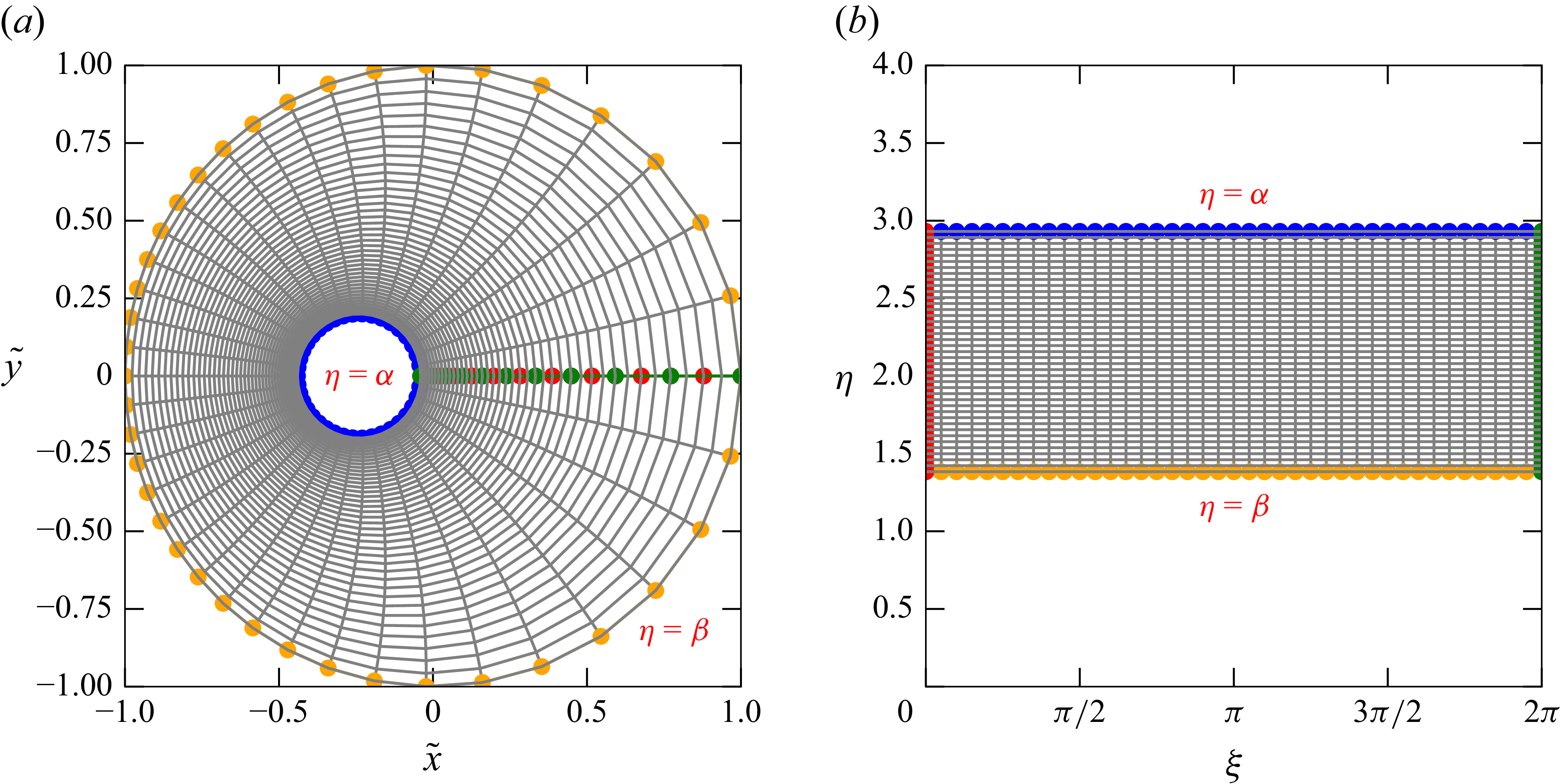
. Figure 2 shows how the physical domain is transformed into a rectangular and uniform computational domain, where the application of the Dirichlet and Neumann boundary conditions is straightforward in both analytical and numerical solutions. The results obtained from the computational domain, figure 2(b), are represented in the physical domain, where, for convenience, the outer cylinder is centred at the origin, as can be shown in figure 2(a) by subtracting the
 $\tilde {x}$
-coordinate of the centre,
 $\tilde {a}\coth \beta$
, from the equation that defines the
 $\tilde {x}$
-axis in (2.14).
Bipolar coordinate transformation. (a) Physical domain: mesh presented in the Cartesian coordinate system (
 $\tilde {x}$
,
 $\tilde {y}$
), where the numerical results are visualised and the boundaries of the domain are indicated by constant values of
 $\alpha$
and
 $\beta$
, which correspond to the
 $\eta$
-coordinate in the bipolar coordinate system. (b) Computational domain: mesh presented in the bipolar coordinate system (
 $\xi$
,
 $\eta$
) where the numerical computations are carried out. Both meshes are shown for illustration purposes only.

To apply the transformation of the governing equations within this computational domain, the spatial term, defined by the Laplacian operator, is expressed in its bipolar coordinates form (Morse & Feshbach Reference Morse and Feshbach1953; Spiegel & Liu Reference Spiegel and Liu1999)
 \begin{equation} {\nabla} _{\xi ,\eta }^{2} = \left (\frac {\zeta }{\tilde {a}}\right )^{2}\left (\frac {\partial ^{2} }{\partial \xi ^{2} } + \frac {\partial ^{2} }{\partial \eta ^{2} }\right ) ,\end{equation}
where
 $\zeta = \cosh \eta - \cos \xi$
. Thus, the Cartesian governing equations are transformed to bipolar coordinates.
In this analysis, we introduce the following dimensionless variables for the momentum equation:
 \begin{equation} W = \frac {\tilde {w}}{\tilde {w}_{c}}, \quad z = \frac {\tilde {z}}{\tilde {\ell }}, \quad t = \tilde {t}\tilde {\omega }, \quad a = \frac {\tilde {a}}{\tilde {r}_{2}}, \end{equation}
where
 $\tilde {w}_c = ({\tilde {G}_0 {\tilde {r}_{2}}^{2}}/{\tilde {\mu }})$
is the characteristic velocity of the flow. By transforming (2.11) into bipolar coordinates, considering the pressure gradient as defined in (2.1) and using the dimensionless variables defined in (2.20), we obtain the corresponding dimensionless momentum equation as follows:
 \begin{equation} {\textit{Wo}}^{2}\left ({\textit{De}}\frac {\partial ^2 W}{\partial t^2} + \frac {\partial W}{\partial t}\right ) = \left (\frac {\zeta }{a}\right )^{2}\left (\frac {\partial ^{2} W}{\partial \xi ^{2} } + \frac {\partial ^{2} W}{\partial \eta ^{2} }\right ) + \left (1 + {\textit{De}}\frac {\partial }{\partial t} \right )\Bigl (1 + g {\textrm{Re}}\Bigl \{ e^{-it} \Bigr \} \Bigr ). \end{equation}
The dimensionless boundary conditions for (2.21) corresponding to the time-harmonic oscillatory flow are
 \begin{align} W = 0 \quad \text{at} \quad \eta &= \alpha \quad \textrm{and} \quad \eta = \beta , \end{align}
 \begin{align} \frac {\partial W}{\partial \xi } = 0 \quad \text{at} \quad \xi &= 0 \quad \textrm{and} \quad \xi = \pi . \end{align}
As a result of the coordinate transformation, the no-slip boundary condition is applied at constant values of the radial coordinate
 $\eta$
corresponding to the inner and outer surfaces. Moreover, the symmetry condition at the mid-plane
 $\tilde {y} = 0$
can be reformulated in terms of the angular coordinate
 $\xi$
, where
 $\xi = 0$
and
 $\xi = \pi$
are about the mid-plane in the bipolar coordinate system.
In this context,
 \begin{equation} {\textit{Wo}} = \sqrt {\frac {\tilde {\omega }\tilde {r}_{2}^2}{\tilde {\nu }}} \end{equation}
is the Womersley number (Womersley Reference Womersley1955a
,
Reference Womersleyb
) that represents the competition between inertial and viscous forces (Pande, Wang & Christov Reference Pande, Wang and Christov2023);
 $\tilde {\nu }$
is the kinematic viscosity of the fluid and
 ${\textit{De}} = \tilde {\lambda } \tilde {\omega }$
is the Deborah number and represents the ratio of the fluid relaxation time to the residence time in the tube. If
 ${\textit{De}} = 0$
, it is a purely viscous fluid, and
 ${\textit{De}} \rightarrow \infty$
is an elastic solid (Rudolph & Osswald Reference Rudolph and Osswald2014).
For the convection-diffusion relation, (2.12), we propose the following dimensionless variables:
 \begin{equation} C = \frac {\tilde {C}}{\tilde {C}_{c}}, \quad t = \frac {\tilde {t}}{{\tilde {r}_2}^2/\tilde {D}}, \quad \end{equation}
where
 $\tilde {C}_{c}$
is the characteristic concentration, and for the transport of the solute, the characteristic time corresponds to the time that the solute is diffused in the radial direction of the tube. The resulting dimensionless advection-diffusion transport (2.12) in bipolar coordinates is the following:
 \begin{equation} \frac {\partial C}{\partial t} + \epsilon {\textit{Pe}} W \frac {\partial C}{\partial z} = \left (\frac {\zeta }{a}\right )^{2}\left (\frac {\partial ^{2} C}{\partial \xi ^{2} } + \frac {\partial ^{2} C}{\partial \eta ^{2} }\right ) + \epsilon ^{2}\frac {\partial ^{2} C}{\partial z^{2}}. \end{equation}
In (2.26),
 ${\textit{Pe}}= \tilde {r}_{2}\tilde {w}_{c}/\tilde {D}$
is the Péclet number, which measures the competition between convective and diffusive transport and
 $\epsilon = \tilde {r}_{2}/\tilde {\ell }$
is the aspect ratio.
The boundary conditions for (2.26), similarly to those applied to the momentum equation in the bipolar coordinate system, consist of impermeability at fixed values of
 $\eta$
and symmetry about the mid-plane. These are imposed as follows:
 \begin{align} \frac {\partial C}{\partial \eta } = 0 \quad \text{at} \quad \eta &= \alpha \quad \text{and} \quad \eta = \beta , \end{align}
 \begin{align} \frac {\partial C}{\partial \xi } = 0 \quad \text{at} \quad \xi &= 0 \quad \text{and} \quad \xi = \pi . \end{align}
Regarding the initial condition, a known function
 $\psi (\xi , \eta ,z)$
is imposed (Taghizadeh, Valdés-Parada & Wood Reference Taghizadeh, Valdés-Parada and Wood2020)
 \begin{equation} C\left (\xi , \eta , z, t = 0 \right ) = \psi \left (\xi ,\eta ,z \right )\!. \end{equation}
Within the framework of homogenization theory, the objective is to derive an averaged equation that captures the long-time behaviour of (2.26). To ensure the problem is fully defined, the condition (2.29) is imposed. Here, it simply states that the initial concentration is known, while the appropriate formulation of the averaged initial condition will be applied in the second-order perturbation problem from the asymptotic analysis (Ng Reference Ng2006).
3. Numerical solution of the momentum equation
Since (2.21) is linear, we can express the pulsatile velocity profile as follows Leal (Reference Leal2007):
 \begin{equation} W\left (\xi ,\eta ,t\right ) = W_{s}\left (\xi ,\eta \right ) + W_{\omega }\left (\xi ,\eta ,t \right )\!. \end{equation}
In (3.1),
 $ W_s$
is the response to the steady part of the pressure gradient, and
 $ W_{\omega }$
is the response to the transient, oscillatory part. Substituting (3.1) into (2.21), we obtain the following two problems:
 \begin{equation} \left (\frac {\zeta }{a}\right )^{2}\left (\frac {\partial ^{2} W_{s}}{\partial \xi ^{2} } + \frac {\partial ^{2} W_{s}}{\partial \eta ^{2} }\right ) + 1 = 0, \end{equation}
and
 \begin{equation} {\textit{Wo}}^{2}\left ({\textit{De}}\frac {\partial ^2 W_{\omega }}{\partial t^2} + \frac {\partial W_{\omega }}{\partial t} \right ) = \left (\frac {\zeta }{a}\right )^{2}\left (\frac {\partial ^{2} W_{\omega }}{\partial \xi ^{2} } + \frac {\partial ^{2} W_{\omega }}{\partial \eta ^{2} }\right ) + \left (1 + {\textit{De}}\frac {\partial }{\partial t} \right )\left (g {\textrm{Re}} \biggl \{e^{-i t} \biggr \} \right )\!. \end{equation}
Equation (3.3) will be solved by proposing the following oscillatory flow solution:
 \begin{equation} W_{\omega } \left (\xi , \eta , t \right ) = {\textrm{Re}} \big \{H\left (\xi ,\eta \right )e^{-i t}\big \}. \end{equation}
Substituting (3.4) into (3.3), yields
 \begin{equation} -{\textit{Wo}}^{2}H\left (i + {\textit{De}}\right ) = \left (\frac {\zeta }{a} \right )^{2}\left (\frac {\partial ^{2}H}{\partial \xi ^{2}} + \frac {\partial ^{2}H}{\partial \eta ^{2}}\right ) + g \left (1 - i{\textit{De}} \right )\!. \end{equation}
Equations (3.2) and (3.5) are solved using the alternating-direction implicit (ADI) technique in combination with the Crank–Nicolson method for the finite-difference framework (John & Anderson Reference John and Anderson1995; Chapra et al. Reference Chapra2011). To numerically solve these equations using the ADI scheme, a fictitious time was introduced with a time step of
 $\Delta t = 1 \times 10^{-2}$
, and a convergence tolerance of
 $tol = 1\times 10^{-8}$
. The computational domain was discretised using a structured mesh comprising
 $90\,000$
nodes. All simulations were implemented in Python.
4. Homogenization theory by multiple scales for the convection-diffusion equation
The dispersion phenomenon presented here involves different time and spatial scales, and we are interested in obtaining the effective dispersion coefficient and how the mean solute concentration is dispersed along the channel for the long-time scale. To achieve this, we employ the homogenization technique (Mei & Vernescu Reference Mei and Vernescu2010; Muñoz et al. Reference Muñoz, Arcos, Bautista and Méndez2018), along with the multiple-scale method, which enables the derivation of effective coefficients and macrotransport equations by averaging from the microscale. In this case, the microscale is defined by the phenomenon of diffusion through the cross-section of the channel, which occurs on a time scale smaller than that of longitudinal transport.
In (2.26), the aspect ratio
 $\epsilon$
is considered to be a very small parameter due to the differing spatial scales involved. To account for this, we perturb the convective-diffusion equation using this parameter and employ multiple-scale analysis. In examining the dispersion phenomenon through (2.26), we identify three distinct time scales: the first is
 $\tilde {r}_{2}^{2}/\tilde {D}$
, representing radial diffusion, which assumes that the diffusion process in that direction is completed within a few periods (
 ${2 \pi }/{\tilde {\omega }} \sim {\tilde {r}_{2}^{2}}/{\tilde {D}}$
); the others are
 $\tilde {\ell }/\tilde {w}_c$
and
 $\tilde {\ell }^2/\tilde {D}$
which describe convection and the diffusion along the length
 $\tilde {\ell }$
. Therefore, we introduce the three time coordinates
 \begin{equation} t_{0} = t,\quad t_{1} = \epsilon t, \quad t_{2} = \epsilon ^{2}t . \end{equation}
In the limit of low frequencies, this assumption is no longer valid, and a different asymptotic analysis would be required, such as that described by Ng (Reference Ng2006), where it is shown that in this regime the oscillation period becomes comparable to the intermediate time scale associated with convective transport.
Following with this analysis, we assume an expansion for the concentration in the form
 \begin{equation} C = C_{0} + \epsilon C_{1} + \epsilon ^{2}C_{2} + \boldsymbol{\cdot}s , \end{equation}
where
 $C_{i} = C_{i}(\xi , \eta , z, t_{0}, t_{1}, t_{2} )$
. In the convection-diffusion relation, (2.26), the original time derivative becomes, using the chain rule
 \begin{equation} \frac {\partial }{\partial t} = \frac {\partial }{\partial t_{0}} + \epsilon \frac {\partial }{\partial t_{1}} + \epsilon ^{2}\frac {\partial }{\partial t_{2}}. \end{equation}
Considering the above (4.1)–(4.3), and (2.26), a sequence of perturbation problems is obtained. They are shown in the following subsections.
4.1. Leading order of
 ${\mathcal{O}}({\epsilon }^{0})$

The following problem governs the concentration at the leading order:
 \begin{equation} \frac {\partial C_{0}}{\partial t_{0}} = \left (\frac {\zeta }{a} \right )^{2} \left (\frac {\partial ^2 C_{0}}{\partial \xi ^2} + \frac {\partial ^2 C_{0}}{\partial \eta ^2} \right )\!, \end{equation}
with the corresponding Neumann boundary conditions
 \begin{align} \frac {\partial C_{0}}{\partial \eta } = 0 \quad \text{at} \quad \eta &= \alpha \quad \text{and} \quad \eta = \beta , \end{align}
 \begin{align} \frac {\partial C_{0}}{\partial \xi } = 0 \quad \text{at} \quad \xi &= 0 \quad \text{and} \quad \xi = \pi . \end{align}
Equation (4.4) is solved by separation of variables, resulting in
 \begin{align} C_{0}\left (\xi ,\eta ,z,t_{0},t_{1},t_{2} \right ) &= C_{00}\left (z,t_{1},t_{2} \right ) + \sum _{m=1}^{\infty } \sum _{n=1}^{\infty }C_{mn}e^{-\left (\frac {\zeta }{a}\right )^2\left [ n^{2} + \left ( \frac {m \pi }{\alpha - \beta } \right )^{2}\right ]t_{0}} \nonumber \\&\quad\times \left \{\cos \left ( \frac {m \pi }{\alpha - \beta }\eta \right )+\tan \left (\frac {m\pi }{\alpha - \beta } \alpha \right )\sin \left (\frac {m\pi }{\alpha - \beta }\eta \right ) \right \}. \end{align}
Since we aim to study the phenomenon of dispersion long after the transverse diffusion has concluded, and because the second term of (4.7) decreases exponentially with increasing
 $ t_{0}$
, we can neglect the series part. Therefore, the concentration at the leading order takes the following form:
 \begin{equation} C_{0} = C_{0}\left (z,t_{1}, t_{2} \right )\!. \end{equation}
Equation (4.8) indicates that
 $C_{0}$
only depends on the coordinates
 $z,t_1,t_2$
. Thus, the leading-order (4.4) reduces to
 \begin{equation} \frac {\partial ^2 C_{0}}{\partial \xi ^2} + \frac {\partial ^2 C_{0}}{\partial \eta ^2} = 0. \end{equation}
In this context,
 $C_0$
corresponds to the non-trivial solution of the problem (4.9), (4.5) and (4.6).
4.2. First order
${\mathcal{O}}(\epsilon )$

At
 ${\mathcal{O}}(\epsilon )$
,
 $C_1$
is governed by the following equations:
 \begin{align}& \frac {\partial C_{0}}{\partial t_1} + \frac {\partial C_{1}}{\partial t_{0}} + {\textit{Pe}} W \frac {\partial C_{0}}{\partial z} = \left (\frac {\zeta }{a} \right )^{2} \left (\frac {\partial ^2 C_{1}}{\partial \xi ^2} + \frac {\partial ^2 C_{1}}{\partial \eta ^2}\right )\!, \end{align}
 \begin{align}&\qquad\quad \frac {\partial C_{1}}{\partial \eta } = 0 \quad \text{at} \quad \eta = \alpha \quad \text{and} \quad \eta = \beta , \end{align}
 \begin{align}&\qquad\quad \frac {\partial C_{1}}{\partial \xi } = 0 \quad \text{at} \quad \xi = 0 \quad \text{and} \quad \xi = \pi . \end{align}
By inserting the steady (
 $W_s$
) and oscillatory (
 $W_{\omega }$
) parts of the velocity into (4.10) with the redefinition of time given in (2.25), we obtain that
 \begin{equation} \frac {\partial C_{0}}{\partial t_1} + \frac {\partial C_{1}}{\partial t_{0}} + {\textit{Pe}} W_{s}\frac {\partial C_{0}}{\partial z} + {\textit{Pe}} \, {\textrm{Re}}\left [{\textit{He}}^{-i{\textit{ScWo}}^2 t_{0}} \right ] \frac {\partial C_{0}}{\partial z} = \left (\frac {\zeta }{a} \right )^{2} \left (\frac {\partial ^2 C_{1}}{\partial \xi ^2} + \frac {\partial ^2 C_{1}}{\partial \eta ^2}\right )\!. \end{equation}
Here,
 ${Sc} = \tilde {\nu }/\tilde {D}$
is the Schmidt number, which measures the competition between momentum and mass diffusion. Then, taking its time and transversal area average using the following definitions:
 \begin{align} \bar {f} &= \frac {{\textit{ScWo}}^2}{2\pi }\int _{0}^{\frac {2\pi }{{\textit{ScWo}}^2} } f\left (t_{0} \right )\textrm{d}t_{0}, \end{align}
 \begin{align} \left \langle f \right \rangle &= \frac {1}{{\pi \bigl [{\textrm{csch}}^2}{\beta } - {\textrm{csch}}^2{\alpha }\bigr ]}\int _{\alpha }^{\beta }\int _{0}^{2\pi }\frac {f \left (\eta ,\xi \right ) }{\left (\cosh {\eta } - \cos {\xi } \right )^2}\,\textrm{d}\xi\,\textrm{d}\eta , \end{align}
where
 $\bar {f}$
and
 $\langle f\rangle$
indicate the time and area average of a function, respectively, we obtain the following equation:
 \begin{equation} \frac {\partial C_{0}}{\partial t_{1}} + {\textit{Pe}}\left \langle W_{s}\right \rangle \frac {\partial C_{0}}{\partial z} = 0. \end{equation}
The above expression is only in terms of
 $C_{0}$
, since averaging
 $C_{1}$
on the cross-sectional area removes its dependence on
 $\xi$
and
 $\eta$
, and subsequent time averaging eliminates its dependence on
 $t_{0}$
. Thus, the derivatives of
 $\bar {C}_{1}$
and
 $\langle C_{1} \rangle$
with respect to
 $t_{0}$
and the cross-sectional area vanish. Consequently, this first-order concentration is eliminated from (4.13).
After subtracting (4.16) from (4.13), we find
 \begin{equation} \frac {\partial C_{1}}{\partial t_{0}} + {\textit{Pe}} \left \{\bar {W}_{s} + {\textrm{Re}}\left [{\textit{He}}^{-i{\textit{ScWo}}^{2}t_{0}} \right ]\right \}\frac {\partial C_{0}}{\partial z} = \left (\frac {\zeta }{a} \right )^{2} \left (\frac {\partial ^2 C_{1}}{\partial \xi ^2} + \frac {\partial ^2 C_{1}}{\partial \eta ^2} \right )\!. \end{equation}
Here,
 $\bar {W}_s = W_s - \langle W_s \rangle$
is the velocity deviation. Since (4.17) is linear, we can propose a solution of the form
 \begin{equation} C_{1} = {\textit{Pe}} \left \{B_{s} + {\textrm{Re}}\left [B_{\omega }e^{-i{\textit{ScWo}}^{2}t_{0}} \right ] \right \}\frac {\partial C_{0}}{\partial z}. \end{equation}
This solution leads to the so-called two cell problems (Mei & Vernescu Reference Mei and Vernescu2010), where
 $B_s$
and
 $B_\omega$
are known as cell functions for the steady and oscillatory parts, respectively. For the steady part, we have the following problem:
 \begin{equation} \left (\frac {\zeta }{a} \right )^{2} \left (\frac {\partial ^2 B_{s}}{\partial \xi ^2} + \frac {\partial ^2 B_{s}}{\partial \eta ^2} \right ) = \bar {W}_{s}, \end{equation}
with boundary conditions
 \begin{align}& \frac {\partial B_{s}}{\partial \eta } = 0 \quad \text{at} \quad \eta = \alpha \quad \text{and} \quad \eta = \beta ,\\[-11pt]\nonumber\end{align}
 \begin{align}& \frac {\partial B_{s}}{\partial \xi } = 0 \quad \text{at} \quad \xi = 0 \quad \text{and} \quad \xi = \pi . \end{align}
For the oscillatory part, the problem is defined by
 \begin{equation} \left (\frac {\zeta }{a} \right )^{2} \left (\frac {\partial ^2 B_{\omega }}{\partial \xi ^2} + \frac {\partial ^2 B_{\omega }}{\partial \eta ^2} \right ) + i{\textit{ScWo}}^2B_{\omega } = H, \end{equation}
with boundary conditions
 \begin{align}& \frac {\partial B_{\omega }}{\partial \eta } = 0 \quad \text{at} \quad \eta = \alpha \quad \text{and} \quad \eta = \beta ,\\[-11pt]\nonumber\end{align}
 \begin{align}& \frac {\partial B_{\omega }}{\partial \xi } = 0 \quad {at} \quad \xi = 0 \quad \text{and} \quad \xi = \pi . \end{align}
The numerical solutions for calculating
 $B_{s}$
and
 $B_{\omega }$
were obtained using the ADI scheme outlined in § 3.
4.3. Problem of
${\mathcal{O}}(\epsilon ^2)$

The problem resulting from the second-order perturbation is the following:
 \begin{equation} \frac {\partial C_{0}}{\partial t_2} + \frac {\partial C_{1}}{\partial t_{1}} + \frac {\partial C_{2}}{\partial t_{0}} + {\textit{Pe}}W \frac {\partial C_{1}}{\partial z} = \left (\frac {\zeta }{a} \right )^2 \left (\frac {\partial ^2 C_{2}}{\partial \xi ^2} + \frac {\partial ^2 C_{2}}{\partial \eta ^2}\right ) + \frac {\partial ^2 C_{0}}{\partial z^2}. \end{equation}
Substituting (3.1) and (4.18) into (4.25), we get
 \begin{align} &\frac {\partial C_{0}}{\partial t_2} + \frac {\partial C_{2}}{\partial t_{0}} + {\textit{Pe}}^2 \left \{\bar {W}_s + {\textrm{Re}} \left [{\textit{He}}^{-i{\textit{ScWo}}^{2}t_{0}} \right ]\right \} \left \{B_{s} + {\textrm{Re}} \left [B_{\omega }e^{-i{\textit{ScWo}}^2t_0} \right ]\right \} \frac {\partial ^2 C_{0}}{\partial z^2}\nonumber \\&\quad = \left (\frac {\zeta }{a} \right )^2 \left (\frac {\partial ^2 C_{2}}{\partial \xi ^2} + \frac {\partial ^2 C_{2}}{\partial \eta ^2}\right ) + \frac {\partial ^2 C_{0}}{\partial z^2}. \end{align}
Manipulating algebraically (4.26), and taking the time and area average, we obtain an expression for the long-time scale that has the form of pure diffusive transport. Similar to (4.16), the resulting expression does not include second-order concentration, since this variable loses its dependence on
 $t_{0}$
and cross-sectional area
 \begin{equation} \frac {\partial C_{0}}{\partial t_{2}} = {D}_{\textit{eff}}\frac {\partial ^2 C_{0}}{\partial z^2}, \end{equation}
where
 $D_{\textit{eff}} = [1 + {\textit{Pe}}^2 \mathscr{D}_{\textit{eff}}]$
is the effective diffusion coefficient and
 $\mathscr{D}_{\textit{eff}} = \{\mathscr{D}_{s} + \mathscr{D}_{\omega } \}$
is the effective dispersion coefficient that is composed for the steady dispersion coefficient
 \begin{equation} \mathscr{D}_{s} = - \left \langle \bar {W}_s B_s \right \rangle , \end{equation}
and the oscillatory dispersion coefficient
 \begin{equation} \mathscr{D}_{\omega } = - \frac {1}{2}{\textrm{Re}}\left \langle H {B_{\omega }}^{*} \right \rangle , \end{equation}
where in the last equation
 $(*)$
indicates the conjugate of complex number
 $B_{\omega }$
. An expression that combines the convective and diffusion phenomena on the long-time scale can be obtained by multiplying the (4.16) by
 $\epsilon$
and the (4.27) by
 $\epsilon ^{2}$
and then adding the resulting expressions
 \begin{equation} \frac {\partial C_{0}}{\partial t} + \epsilon {\textit{Pe}}\left \langle W_{s} \right \rangle \frac {\partial C_{0}}{\partial z} = \epsilon ^{2} \left [1 + {\textit{Pe}}^{2}\mathscr{D}_{\textit{eff}} \right ]\frac {\partial ^2 C_{0}}{\partial z^{2}}. \end{equation}
As we can appreciate, the above multiple-scale procedure was used to derive (4.30). The determination of the solution for (4.26) is outside of the main objective of this work. Equation (4.30) was solved numerically for
 $C_{0}$
using the Crank–Nicolson method with a time step of
 $\Delta t = 1\times 10^{-4}$
, and
 $z$
-axis discretised by
 $1000$
nodes.
5. Results and discussion
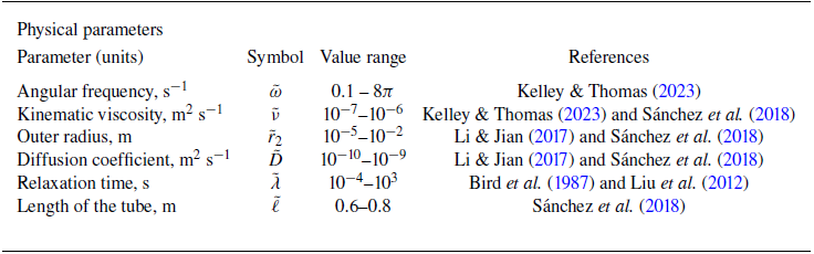
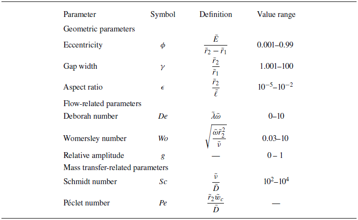
The calculations in this section were carried out using the dimensionless parameters listed in table 2. These parameters were defined based on the physical values given in table 1. All computations in this section were conducted with g = 1. It is also important to emphasise that the results and analysis presented here are applicable only to the selected combinations of parameters listed in table 1, for which the assumption made at the beginning of the homogenization analysis is satisfied, namely that the characteristic time of radial diffusion is of the same order of magnitude as the oscillation period.
Typical values of the dimensional parameters.

Dimensionless parameters involved in the Taylor dispersion problem in an eccentric annular tube.

We begin this section by validating our numerical results against those of previous studies by other authors.
5.1. Validation
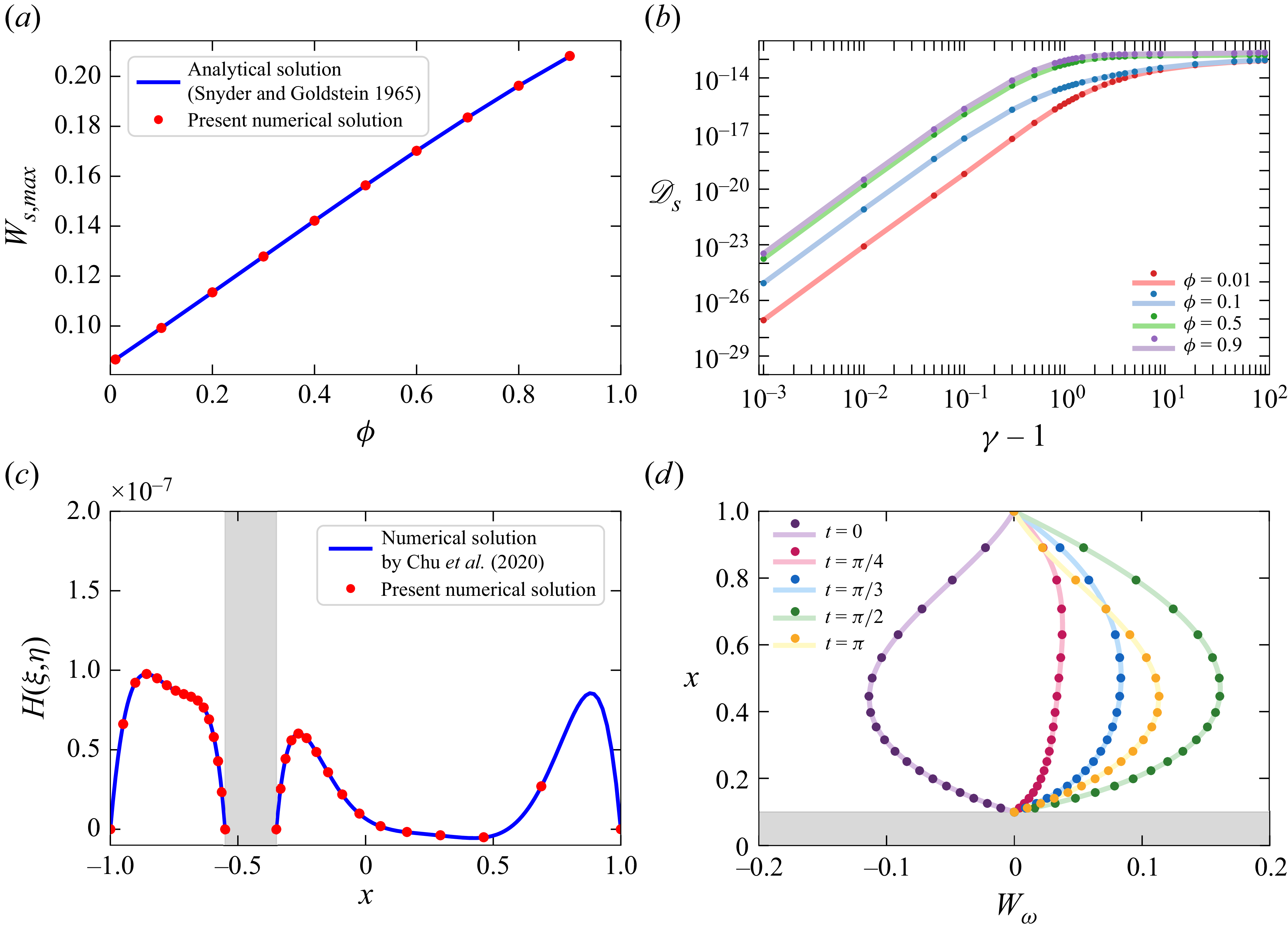
Figure 3(a) displays the maximum velocity obtained from the numerical solution of (3.2). This result is compared with the maximum velocity derived from the exact analytical solution provided by Snyder & Goldstein (Reference Snyder and Goldstein1965). The mathematical expression for the velocity resulting from a constant pressure gradient is detailed in Appendix A. We have replicated their scaling and adjusted their dimensionless velocity by the factor
 $\tilde {a}^{2}/\tilde {r}^{2}_{2}$
, as they non-dimensionalised their velocity using half the distance between the poles rather than the outer radius. An excellent agreement is observed between our numerical results and the data from the exact analytical solution.
Validation. In all the subplots shown, the solid lines correspond to the different authors cited, while the circle markers correspond to the numerical results of the present work. (a) Steady velocity: maximum value of velocity as a function of eccentricity for
 ${\textit{De}} = 0$
and
 $\gamma = 5$
. (b) Steady dispersion coefficient:
 $\mathscr{D}_{s}$
as function of the gap width for different values of eccentricity and
 ${\textit{De}}=0$
. (c) Oscillatory velocity: function
 $H$
as a function of
 $x$
-coordinate at
 $y=0$
for
 ${\textit{De}} = 0$
,
 ${\textit{Wo}} = 10$
,
 $\phi = 5$
and
 $\gamma = 10$
. (d) Rheological model: oscillatory velocity as a function of
 $x$
-coordinate at
 $y = 0$
for
 ${\textit{De}} = 1$
,
 ${\textit{Wo}}= 3$
,
 $\gamma = 10$
and
 $\phi = 0.001$
. All computations were carried out for
 $g = 1$
.

To further validate the contribution of the steady component, figure 3(b) presents data acquired by numerically solving (3.2), (4.19) and (4.28) from which the steady dispersion coefficient is obtained, along with the momentum and steady canonical cell equations provided by Chu et al. (Reference Chu, Garoff, Tilton and Khair2020) (see Appendix A) in their study. It is worth noting that they carried out their analysis of dispersion in a pulsatile flow with a Newtonian fluid through an eccentric annular tube. Although they utilised a different method of non-dimensionalisation, we successfully recovered their solution. Our dimensionless velocity is related to theirs by a factor of
 $\epsilon ^{2}$
because they scaled the dimensionless velocity with the channel length rather than the outer radius. Given the strong agreement between our results, we can confirm that the steady component of our numerical solution is validated.
The contribution of the oscillatory component was validated against the results from Chu et al. (Reference Chu, Garoff, Tilton and Khair2020), using the same equation solved for the steady state (see Appendix A). In this case, the parameters defining the oscillatory behaviour were maintained in the analysis. We compared these numerical results with data obtained by solving (3.5), which offers a solution for the function
 $H$
defined by the phasor in (3.4). By comparing the Womersley number with their dimensionless parameter for angular frequency, we were able to replicate their results (they reported computations with
 ${Sc} = 10^{3}$
). As shown in figure 3(c), there is a strong agreement in this comparison.
To conclude the validation, we present in figure 3(d) the validity of our proposed rheological model. This is done by comparing the numerical results obtained from solving (3.5) for the function
 $H$
, followed by solving (3.4) to obtain the oscillatory velocity at dimensionless periodic times of
 $0$
,
 ${\pi }/{4}$
,
 ${\pi }/{3}$
,
 ${\pi }/{2}$
and
 $\pi$
. These results were compared with those in Barrera et al. (Reference Barrera, Arcos, Mèndez and Bautista2025), who developed an exact analytical solution for Jeffreys’ rheological model in concentric annuli. From this constitutive equation, we can recover Maxwell’s rheological model. Additionally, from our analysis of the eccentric geometry, we can derive an approximate concentric geometry with an eccentricity of
 $\phi = 0.001$
. Despite this concentric approximation, our numerical formulation closely matches the results of Barrera et al. (Reference Barrera, Arcos, Mèndez and Bautista2025).
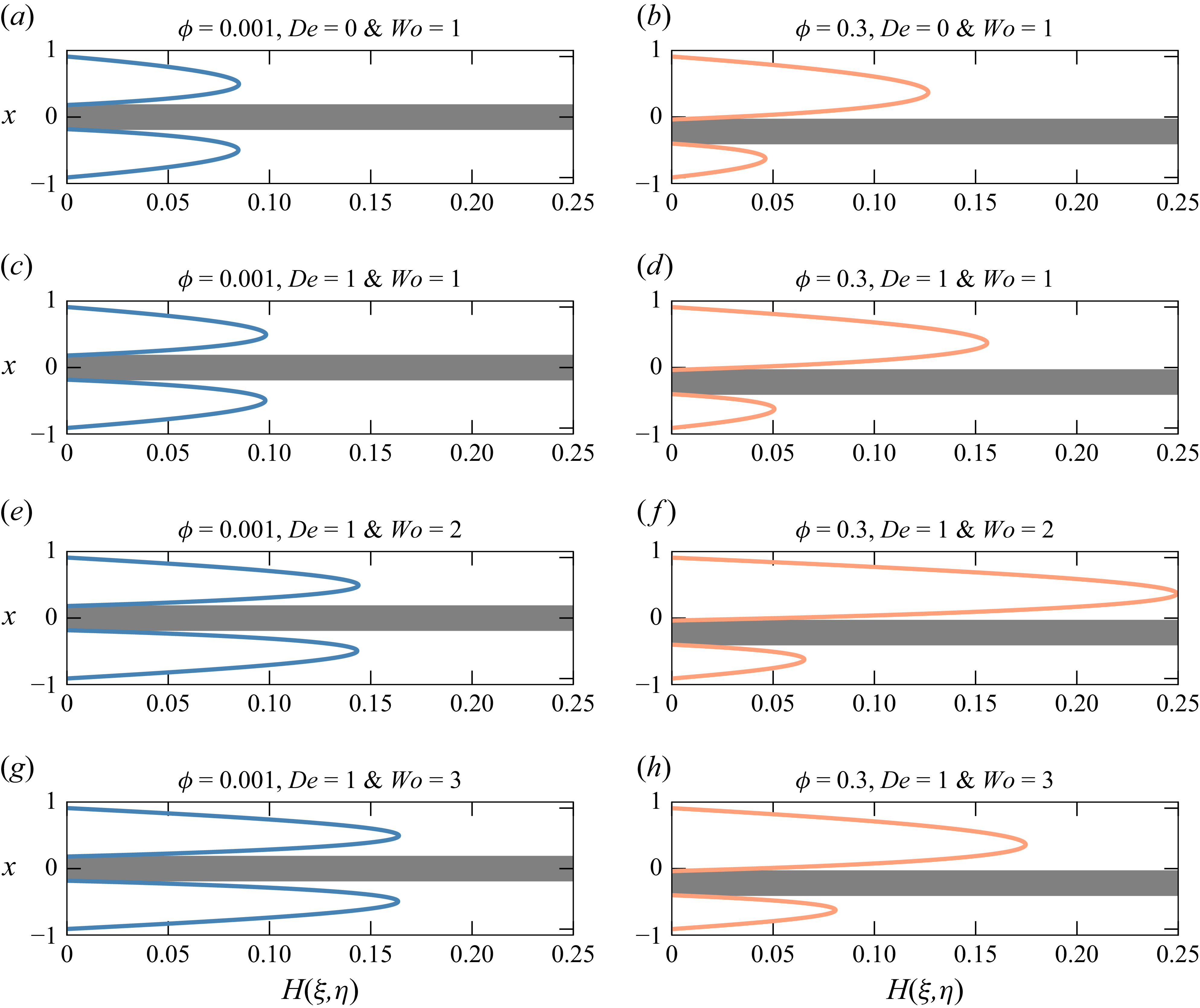
Effect of viscoelasticity on oscillatory velocity in an eccentric annulus. The function
 $H$
as a function of
 $x$
-coordinate at
 $y = 0$
. The function
 $H$
is related to the oscillatory velocity through (3.4). All computations were carried out for
 $\gamma = 5$
and
 $g = 1$
.

5.2. Velocity profile of a viscoelastic fluid
The superposition of the velocity profile into its steady and oscillatory components reveals that the effect of viscoelasticity is solely present in the oscillatory part (
 $W_{\omega }$
), which is the time-dependent component. The above is a consequence of using the linear Maxwell model. Figure 4 illustrates how viscoelasticity affects the oscillatory velocity profiles, using the function
 $H$
as a reference for the oscillatory contribution. The plots on the left feature the same parameters as those on the right, with the key difference being that the left side approaches a concentric configuration (
 $\phi = 0.001$
), while the right side represents an eccentricity of
 $\phi = 0.3$
. This figure demonstrates how both eccentricity and viscoelasticity influence the velocity profile for purely oscillating flow and pulsatile flow (which results from a combination of steady and oscillatory velocities).
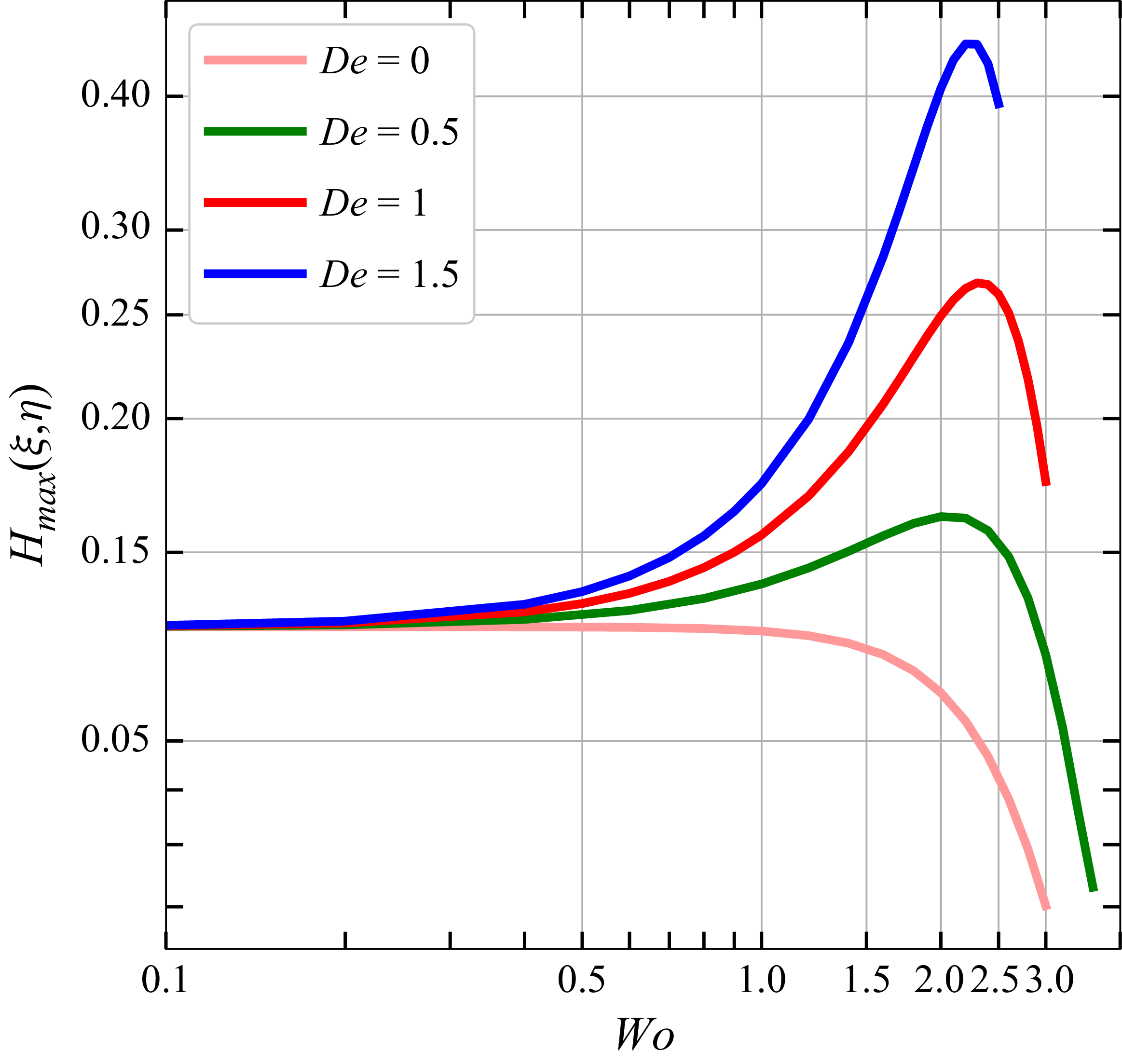
Figure 4(a–b) corresponds to the findings of Snyder & Goldstein (Reference Snyder and Goldstein1965) and Sankarasubramanian & Gill (Reference Sankarasubramanian and Gill1971), which indicate that increasing eccentricity enhances the velocity in an annulus. These observations also hold true for viscoelastic fluids, as shown in figure 4(c–d). Moreover, the effect of viscoelasticity further contributes to this improvement. Figure 4(e–h) highlights a significant characteristic of viscoelastic oscillatory flows: at low frequencies, the velocity exhibits only a slight increase; however, beyond the Womersley number of
 ${\textit{Wo}} = 0.5$
(see figure 5), viscoelasticity has a pronounced impact. Specifically, after this threshold value of
 ${\textit{Wo}}$
, the velocity for viscoelastic fluids increases in a non-monotonic manner. In contrast, for Newtonian fluids, the velocity magnitude consistently decreases. This behaviour is illustrated in figure 5, where the Newtonian fluid demonstrates a steady linear decay. Thus, while the oscillatory velocity increases with the Deborah number at low frequencies, it decays at a certain value of Womersley number.
Maximum value of
 $H$
as a function of
 ${\textit{Wo}}$
for different values of
 ${\textit{De}}$
 $(0,0.5,1,1.5)$
. All computations were carried out for
 $g = 1$
,
 $\gamma = 5$
and
 $\phi = 0.3$
.

5.3. Start-up flow
The interesting behaviour observed in figure 5 has been reported previously by other authors (Andrienko, Siginer & Yanovsky Reference Andrienko, Siginer and Yanovsky2000; Castrejón-Pita et al. Reference Castrejón-Pita, Del Río, Castrejón-Pita and Huelsz2003; Yin & Zhu Reference Yin and Zhu2006; Yang et al. Reference Yang, Christov, Griffiths and Ramon2020). In those studies, as the Womersley number increases, distinct peaks in the velocity magnitude appear at specific values of
 ${\textit{Wo}}$
. Yang et al. (Reference Yang, Christov, Griffiths and Ramon2020) referred to this phenomenon as viscoelastic resonance and defined the specific values of
 ${\textit{Wo}}$
at which the velocity is amplified as the dimensionless resonant frequencies.
With reference to table 2, our analysis focuses on low values of the Deborah and Womersley numbers. However, to capture the different resonance peaks reported by the previously cited authors, this study would need to be extended to larger values of
 ${\textit{De}}$
and
 ${\textit{Wo}}$
. Because the velocity profile is decomposed into its steady and oscillatory components, with
 $W_{\omega }$
proposed as a phasor, numerical instabilities arise for large values, leading to divergence of the solution.
To address this problem, we propose an alternative numerical approach to (2.21) in order to obtain solutions over a wide range of Deborah and Womersley numbers. Since the ADI scheme cannot be directly applied to this second-order hyperbolic partial differential equation, following the work of Araújo et al. (Reference Araújo, Neves and Sousa2014), an auxiliary function,
 $S = {\textit{Wo}}^{2} ({\textit{De}} (\partial W/\partial t) + W )$
, is introduced to reduce the order of the original equation. Consequently, (2.21) can be rewritten as
 \begin{equation} \frac {\partial S}{\partial t} = \left (\frac {\zeta }{a}\right )^{2}\left (\frac {\partial ^{2} W}{\partial \xi ^{2} } + \frac {\partial ^{2} W}{\partial \eta ^{2} }\right ) + \left (1 + {\textit{De}}\frac {\partial }{\partial t} \right )\Bigl (1 + g {\textrm{Re}}\Bigl \{ e^{-it} \Bigr \} \Bigr ). \end{equation}
The reduced (5.1), together with the boundary conditions defined in (2.22) and (2.23), and subject to the initial condition
 $W = 0$
at
 $t = 0$
, is solved using the ADI scheme. The auxiliary function is discretised using the Crank–Nicolson method. Both equations are solved simultaneously on a mesh of
 $90,000$
nodes, with a time step of
 $\Delta t = 1 \times 10^{-4}$
and a convergence tolerance of
 $tol = 1 \times 10^{-6}$
. This approach is based on the solution of the unsteady momentum equation in its complete form, including the time-dependent terms, corresponding to a pulsatile flow from start-up. In the following, we focus on the oscillatory velocity component,
 $W_{\omega }$
, attained once the flow reaches a periodic state. Accordingly, the pressure gradient is prescribed as
 $\tilde {G} = \tilde {G}_{0}\, {\textrm{Re}}\{ e^{-i\tilde {\omega }\tilde {t}} \}$
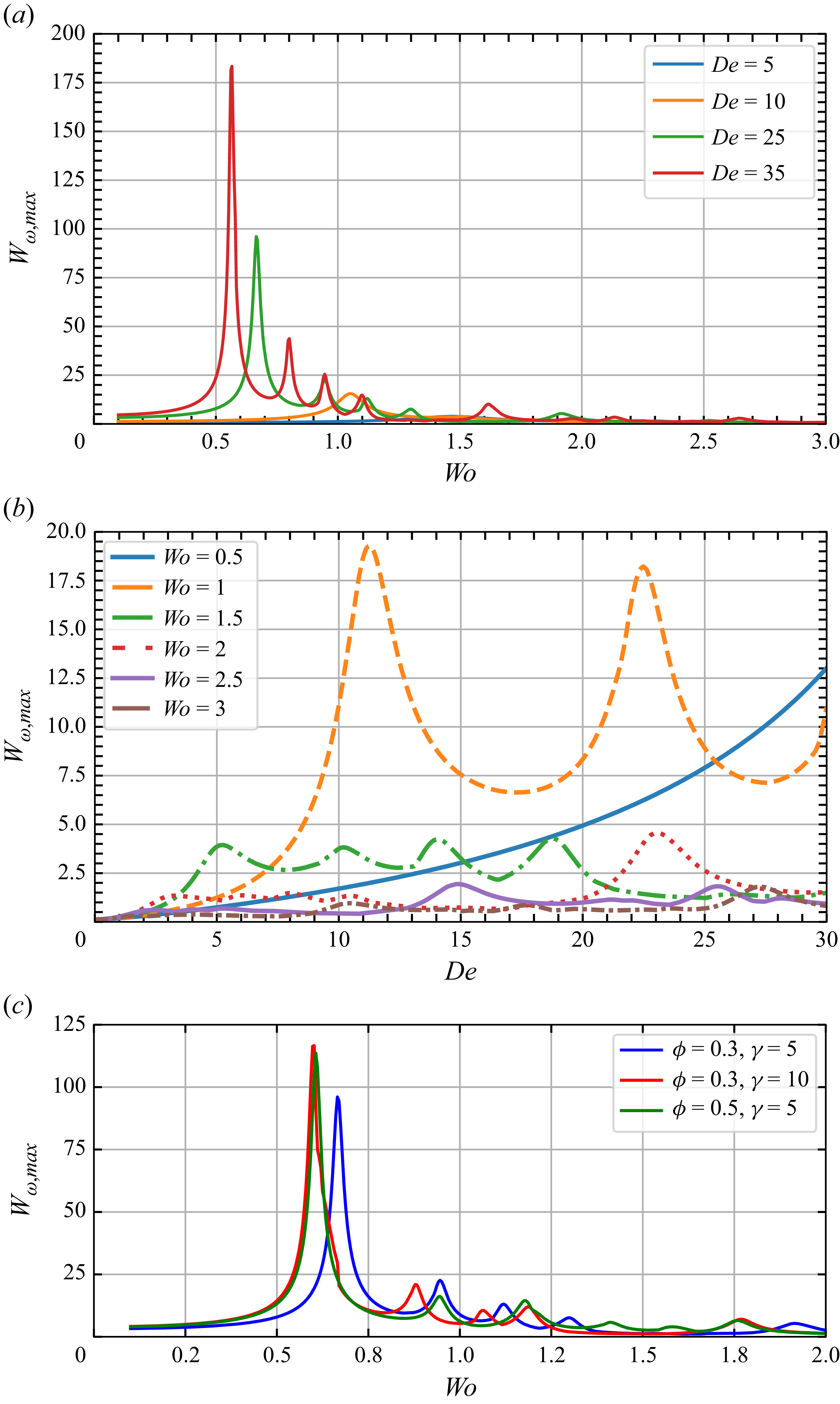
. Most of the aforementioned works, whether analytical or experimental, present plots similar to figure 6(a), where the velocity magnitude is shown as a function of frequency. In our case, the maximum velocity reached by the fluid during one oscillation period is plotted against the Womersley number for different Deborah numbers. The results obtained are consistent with those previously reported, showing that the largest enhancement in the oscillatory velocity occurs at the lowest resonance frequency, and that the magnitude of these resonance peaks decreases as the frequency increases (Andrienko et al. Reference Andrienko, Siginer and Yanovsky2000). This figure also shows that, as the Deborah number increases, the amplitude of the resonance peaks grows significantly, while the corresponding resonance frequencies shift to lower values. Figure 6(b) presents the maximum oscillatory velocity as a function of the Deborah number for different values of
 ${\textit{Wo}}$
. A clear correspondence can be observed between this figure and figure 6(a): at low frequencies, the velocity magnitude increases from the curve of
 ${\textit{Wo}} = 0.5$
to
 ${\textit{Wo}} = 1$
, and beyond this value it decreases continuously. Similarly, peaks in velocity magnitude are identified at specific Deborah numbers, and only at low frequencies, i.e. for
 ${\textit{Wo}} = 0.5$
, a continuous increase in velocity magnitude is observed as
 ${\textit{De}}$
increases. For higher values of
 ${\textit{Wo}}$
the behaviour becomes non-monotonic and does not follow a consistent trend. Depending on the chosen Womersley number, the curves display distinct trends, although it can be highlighted that there exist specific Deborah numbers at which the oscillatory velocity is increased. The objective of figure 6(c) is to illustrate the effect of eccentricity and gap width on the viscoelastic resonance phenomenon. It is observed that, compared with the simulation performed for a viscoelastic fluid with
 ${\textit{De}} = 25$
,
 $\phi = 0.3$
and
 $\gamma = 5$
, increasing the gap width to
 $\gamma = 10$
leads to a higher amplitude of the oscillatory velocity associated with the first resonance peak, while the corresponding resonant frequency shifts to a lower value. Regarding eccentricity, when
 $\phi$
is increased to
 $0.5$
, the oscillatory velocity is likewise enhanced and the resonant frequency is reduced, showing a behaviour similar to that observed when the gap width is increased.
Maximum value of
 $W_{\omega }$
during one oscillation period: (a) as a function of
 ${\textit{Wo}}$
for different values of
 ${\textit{De}}$
, with
 $g = 1$
,
 $\gamma = 5$
and
 $\phi = 0.3$
; (b) as a function of
 ${\textit{De}}$
for different values of
 ${\textit{Wo}}$
, with
 $g = 1$
,
 $\gamma = 5$
and
 $\phi = 0.3$
; and (c) as a function of
 ${\textit{Wo}}$
for two different values of eccentricity (
 $\phi = 0.5, 0.3$
) and two values of the gap width (
 $\gamma = 5, 10$
) for
 ${\textit{De}} = 25$
and
 $g = 1$
.

5.4. Effect of viscoelasticity on the effective dispersion coefficient
5.4.1. Effective dispersion coefficients as a function of the parameter
$\gamma$

Effective dispersion coefficient as a function of the parameter
 $(\gamma - 1)$
for
 $\phi = 0.3$
and
 $g = 1$
.

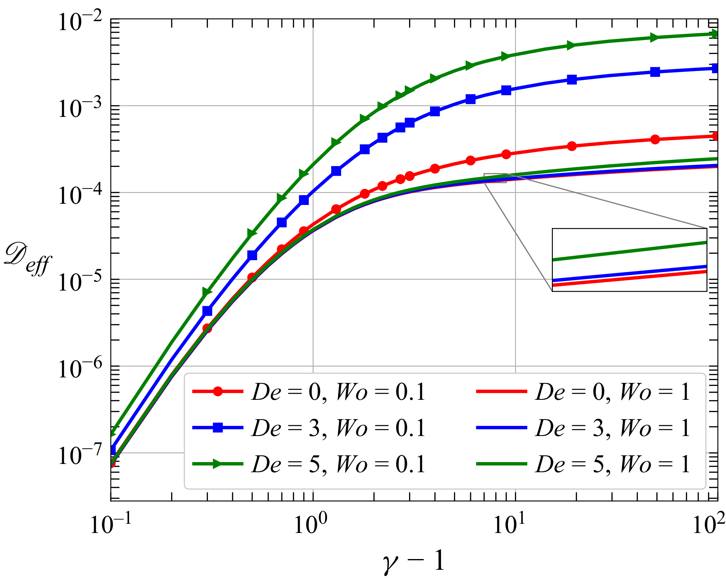
As reported by Sankarasubramanian & Gill (Reference Sankarasubramanian and Gill1971) and Chu et al. (Reference Chu, Garoff, Tilton and Khair2020), the effective dispersion coefficient increases with the gap width, meaning that as the annular gap widens, the dispersion of the solute also increases. These findings are also relevant for viscoelastic fluids. Figure 7 illustrates that effective dispersion enhances with an increase in the Deborah number. This increase can reach up to two orders of magnitude when comparing the dispersion in the pulsatile flow of a Newtonian fluid with that in a viscoelastic fluid with a small Womersley number. Additionally, it is important to note that the viscoelastic impact on the dispersion coefficient due to oscillatory velocity becomes negligible as the Womersley number increases, for example, at
 ${\textit{Wo}} = 1$
. Chu et al. (Reference Chu, Garoff, Tilton and Khair2020) analysed the scaling of the dispersion coefficients
 $\mathscr{D}_{s}$
and
 $\mathscr{D}_{\omega }$
at small and large gap widths
 $(\gamma - 1)$
. They reported that, for
 $(\gamma - 1)\ll 1$
, the corresponding scaling follows
 $\mathscr{D}_{s} \sim (\gamma - 1)^{6}$
for concentric configurations and
 $\mathscr{D}_{s} \sim (\gamma - 1)^{4}$
for eccentric ones, when the fluid has a Newtonian behaviour. These scalings also apply to
 $\mathscr{D}_{\omega }$
.
In the present work, we assess similar relations through the scaling of the effective dispersion coefficient,
 $\mathscr{D}_{\textit{eff}}$
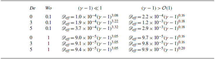
. Figure 7, together with the accompanying table, presents the power-law relationship between
 $\mathscr{D}_{\textit{eff}}$
and
 $(\gamma - 1)$
, expressed as
 $\mathscr{D}_{\textit{eff}} = A (\gamma - 1)^{B}$
. The constants
 $A$
and
 $B$
were obtained by performing a power-law fit to the data shown in figure 7, corresponding to the small and large gap width regimes.
From these results, it is observed that, for
 $(\gamma - 1)\ll 1$
, the exponent
 $B$
is nearly independent of the Deborah and Womersley numbers, with an average value of approximately
 $B \approx 3.1$
. This value is close to the scaling reported by Chu et al. (Reference Chu, Garoff, Tilton and Khair2020) for the steady and oscillatory dispersion coefficients in eccentric configurations (
 $B = 4$
) and for Newtonian fluids. On the other hand, in the large gap width regime, the exponent
 $B$
takes very small values (
 $B \approx 0.16$
–
 $0.20$
), indicating a weak dependence of
 $\mathscr{D}_{\textit{eff}}$
on
 $(\gamma - 1)$
in this limit.
5.4.2. Oscillatory dispersion coefficient
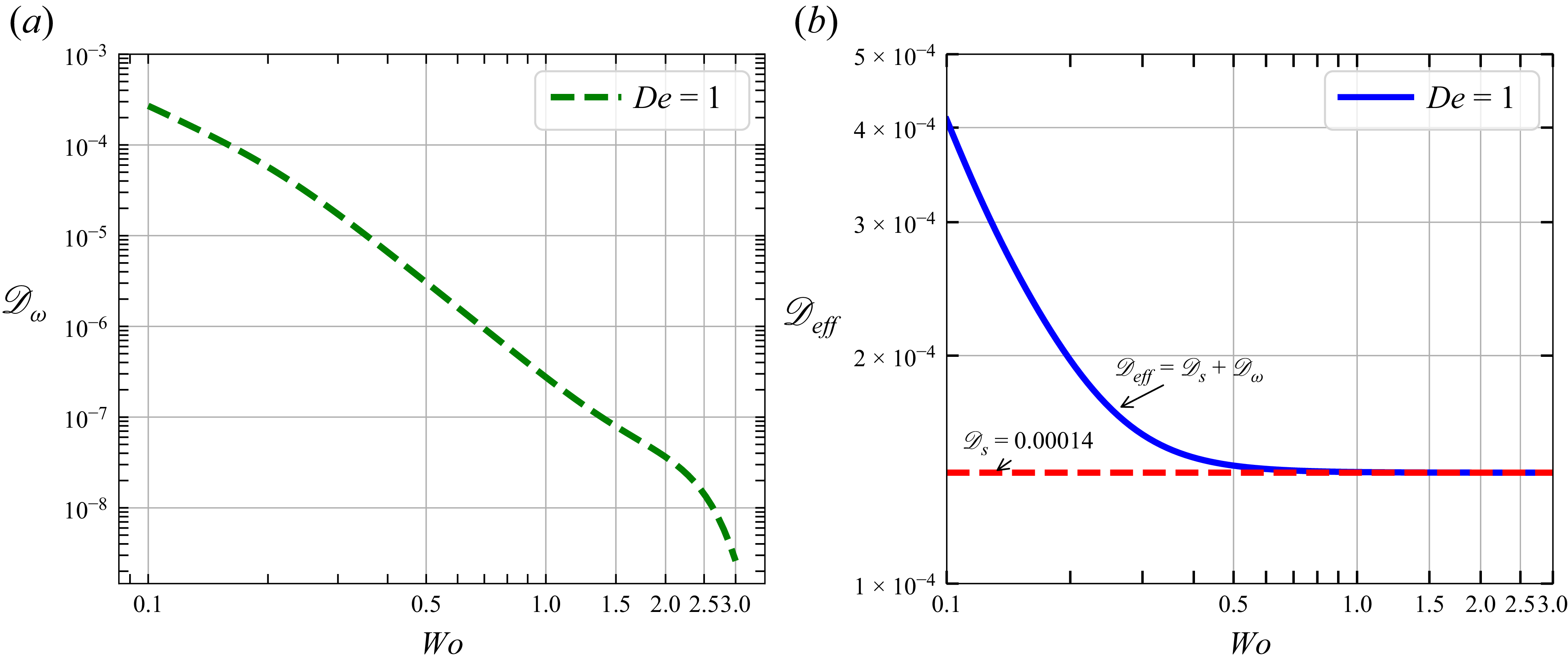
The results presented above highlight the significant influence of the Womersley and Deborah numbers on the dispersion of solutes. Figure 8 illustrates how the oscillatory dispersion coefficient contributes to the effective dispersion coefficient as a function of the Womersley number. A qualitative relationship can be established between figures 8(a) and 5. The oscillatory dispersion coefficient, denoted as
 $\mathscr{D}_{\omega }$
, does not show an increase at low frequencies. This behaviour is further supported by figure 5, which reveals a linear decay regime of
 $\mathscr{D}_{\omega }$
as the magnitude of the function
 $H$
gradually increases, reaching its maximum value at the first resonant frequency. Beyond this point,
 $\mathscr{D}_{\omega }$
exhibits a more pronounced decrease in magnitude as
 ${\textit{Wo}}$
increases. To summarise, the oscillatory dispersion coefficient consistently decreases as the Womersley number increases. As a result, its contribution to the effective dispersion coefficient also diminishes with rising values of
 ${\textit{Wo}}$
, as illustrated in figure 8(b). This is consistent with the findings of Yang et al. (Reference Yang, Christov, Griffiths and Ramon2020), who demonstrated that the effective dispersion coefficient is enhanced near resonance. In the present study, we report results for the effective dispersion coefficient corresponding only to the first and most significant resonant frequency, since our oscillatory velocity solution, proposed as a phasor, exhibits numerical instabilities as
 ${\textit{Wo}}$
and
 ${\textit{De}}$
increase. Nevertheless, based on both our results and those of Yang et al. (Reference Yang, Christov, Griffiths and Ramon2020), we would expect that at higher Womersley numbers, where additional resonant frequencies appear, the dispersion coefficient would not decay as rapidly, although the overall decreasing trend would remain, as described in figure 8(a).
(a) Oscillatory dispersion coefficient and (b) the effective dispersion coefficient as a function of the Womersley number. All computations were carried out for
 $\epsilon = 0.001$
,
 $g = 1$
,
 $\phi = 0.3$
,
 ${Sc} = 10^3$
and
 $\gamma = 10$
.

Effective dispersion coefficient as a function of the Schmidt number, for different values of
 ${\textit{De}}$
, considering
 $\epsilon = 0.001$
,
 $g = 1$
,
 $\phi = 0.3$
,
 $\gamma = 10$
and
 ${\textit{Wo}} = 0.1$
.

5.4.3. Influence of the Schmidt and Deborah numbers on the effective dispersion coefficient
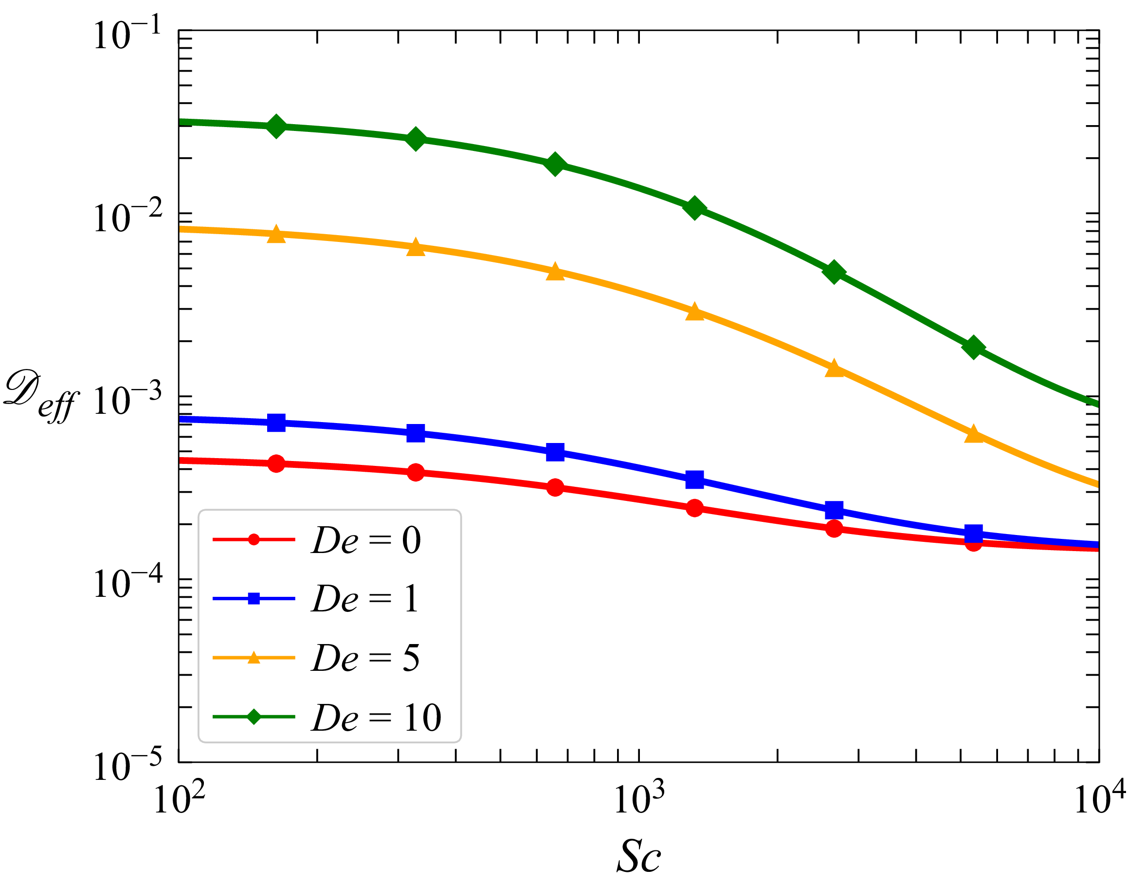
Figure 9 shows a significant enhancement in the effective dispersion coefficient when viscoelastic fluids are employed. This enhancement could be up to three orders of magnitude greater than that of the Newtonian fluid. Besides, the effective dispersion coefficient decreases as soon as the Schmidt number exceeds a certain value, where the momentum diffusion becomes more representative than mass diffusion, which leads to a reduction in the dispersion of the solute. These findings have been previously reported by Ng (Reference Ng2006) and Mei & Vernescu (Reference Mei and Vernescu2010), who observed that the effective dispersion coefficients,
 $\mathscr{D}_s$
and
 $\mathscr{D}_{\omega }$
, decrease with increasing
 ${Sc}$
. Furthermore, Ng (Reference Ng2006) noted that, for low values of the Schmidt number and/or the oscillation frequency, the effective oscillatory dispersion coefficient shows no dependence on these parameters.
5.5. Effect of viscoelasticity on the mean concentration at the long-time scale
To describe the behaviour of the concentration for a viscoelastic fluid, we have solved the (4.30) for the mean concentration, which depends only on the axial direction and the long-time scale. Therefore, an initial condition for the mean concentration must be defined by the known function
 $\psi (z)$
which only depends on
 $z$
-axis and, following the works of Bharadwaj, Santiago & Mohammadi (Reference Bharadwaj, Santiago and Mohammadi2002) and Chu et al. (Reference Chu, Garoff, Tilton and Khair2020), we have proposed a mass pulse with the form of a normalised Gaussian distribution in its dimensionless form as
 \begin{equation} \psi (z) = C_{0}\left (z,t =0 \right ) = e^{-\frac {1}{2} \left (\frac {z - z_{0}}{\sigma } \right )^{2}}, \end{equation}
where
 $z_{0}$
denotes the position along the
 $z$
-axis at which the solute is introduced at time
 $t = 0$
, and
 $\sigma$
is the initial standard deviation. For computations,
 $z_{0} = 0.2$
,
 $\sigma = 0.01$
and
 $\epsilon = 0.001$
were chosen. The values of the Péclet number considered in this section are selected according to the range of validity of the solution given in (4.30), which is determined by two fundamental assumptions. By definition, the Péclet number measures the relative importance of convective transport compared with molecular diffusion. Consequently, the range of validity is constrained so that Taylor dispersion exists between the two limiting cases: pure convection and pure molecular diffusion. The first assumption requires that the convective contribution in (4.30),
 $\epsilon {\textit{Pe}}\langle W_{s} \rangle$
, dominates over the Taylor dispersion contribution,
 $\epsilon ^{2}{\textit{Pe}}^{2}\mathscr{D}_\textit{eff}$
. The second assumption requires that the Taylor dispersion term is larger than the molecular diffusion contribution,
 $\epsilon ^{2}$
(Chu et al. Reference Chu, Garoff, Tilton and Khair2020). Together, these conditions define the admissible range of Péclet numbers as follows:
 \begin{equation} \frac {\left \langle W_{s} \right \rangle }{\epsilon \mathscr{D}_{\textit{eff}}}\gt \gt {\textit{Pe}} \gt \gt \sqrt {\frac {1}{\mathscr{D}_{\textit{eff}}}}. \end{equation}
The calculation of dispersion coefficients is sufficient to assess how effectively a solute can be dispersed under given flow conditions and physical fluid properties. In this section, however, we describe how the dispersion coefficients influence the mean concentration and how the roles of eccentricity, types of flow and fluid viscoelasticity enhance dispersion.
Influence of eccentricity on the dispersion of the solute in a Newtonian fluid for different dimensionless times. For a pulsatile flow with
 $\epsilon = 0.001$
,
 $\gamma = 5$
,
 $g = 1$
and
 ${Sc} = 10^{3}$
. An animation of this figure is provided in Supplementary Movie 1.

Viscoelastic influence on the dispersion of the solute for different dimensionless times. For a pulsatile flow with
 $\epsilon = 0.001$
,
 $\gamma = 5$
,
 $g = 1$
and
 ${Sc} = 10^{3}$
. An animation of this figure is provided in Supplementary Movie 2.

Viscoelastic fluid under different flow conditions. For a flow with
 $\epsilon = 0.001$
,
 $\gamma = 5$
,
 $g = 1$
and
 ${Sc} = 10^{3}$
. An animation of this figure is provided in Supplementary Movie 3.

Influence of Péclet number on mean concentration in a pulsatile flow for viscoelastic fluids. Considering
 $\epsilon = 0.001$
,
 $g = 1$
and
 ${Sc} = 10^{3}$
. An animation of this figure is provided in Supplementary Movie 4.

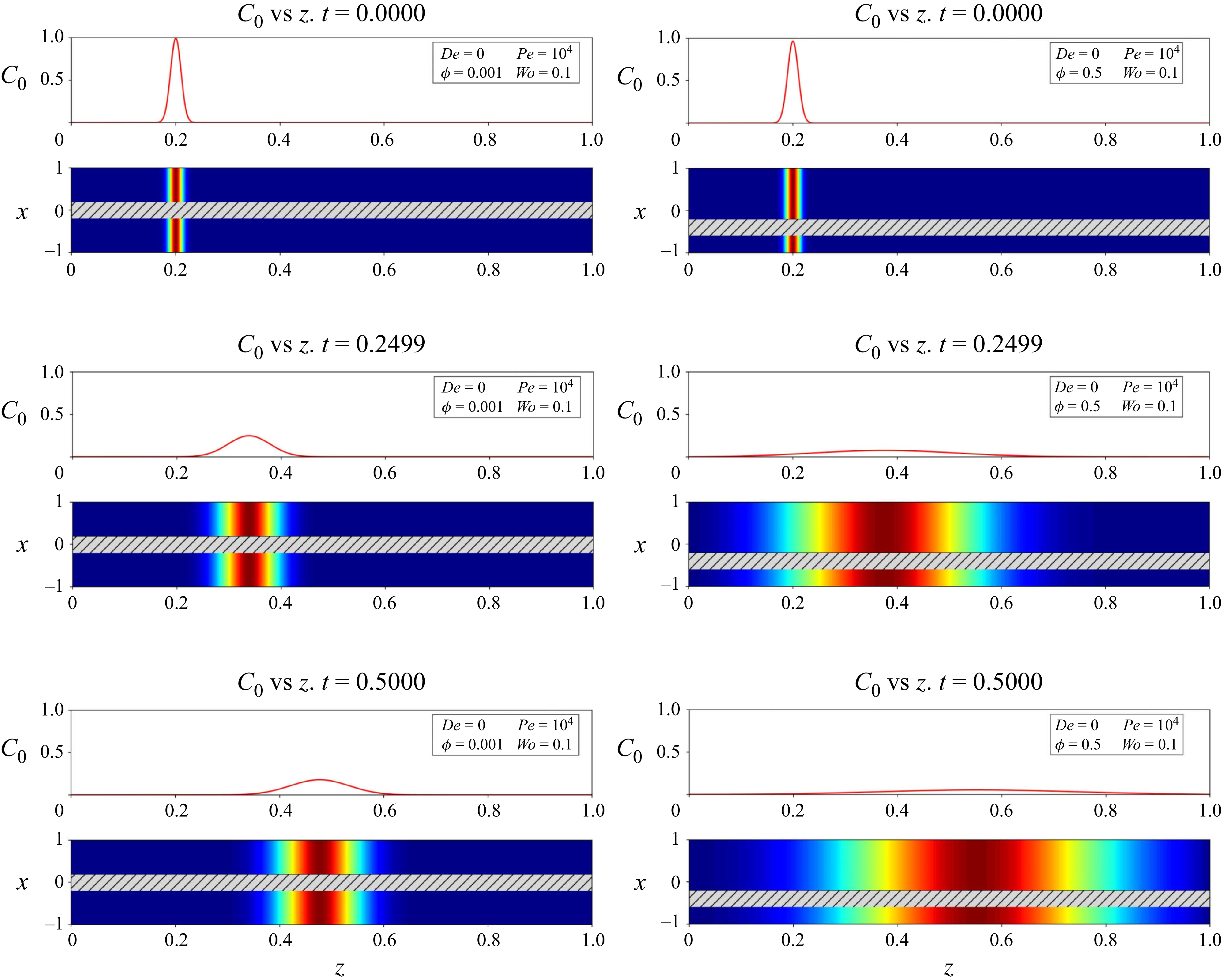
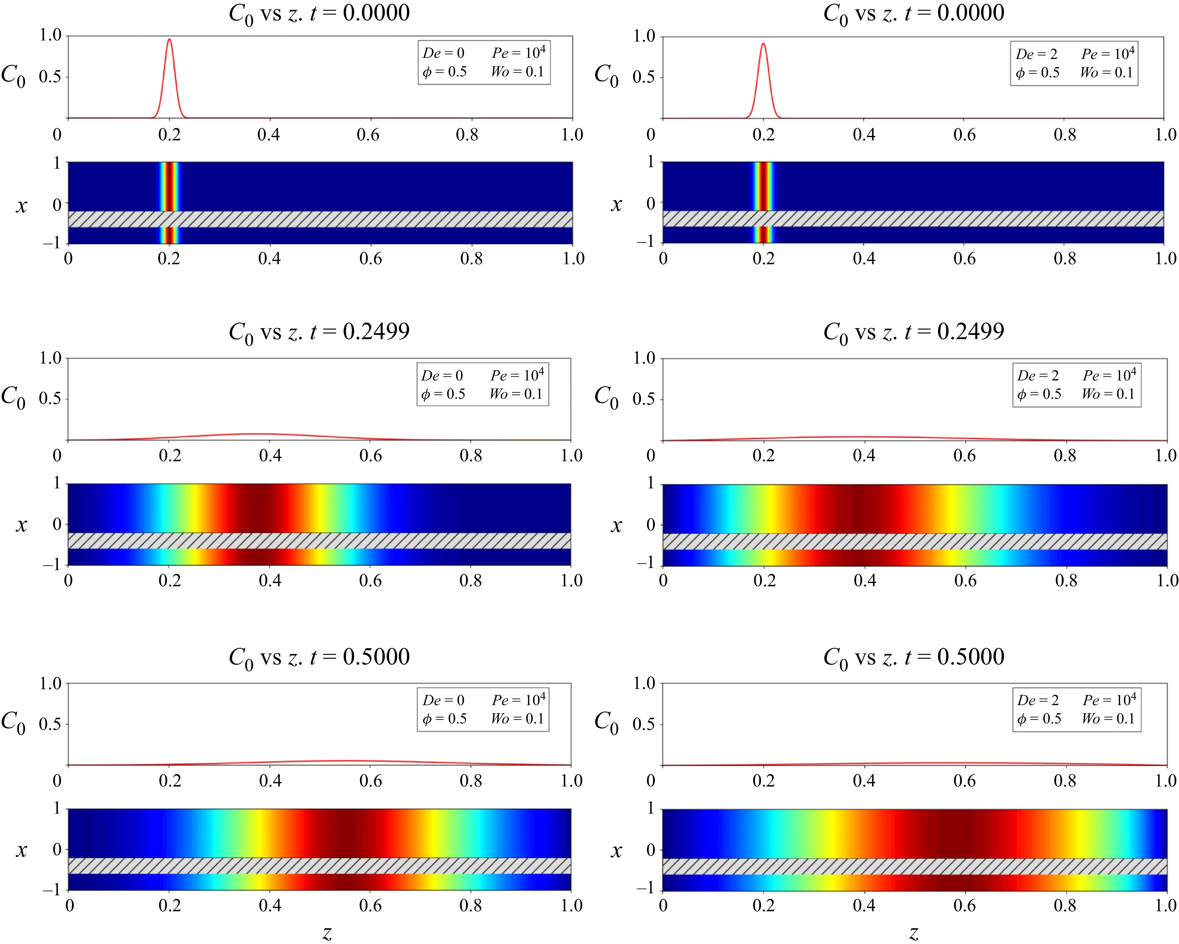
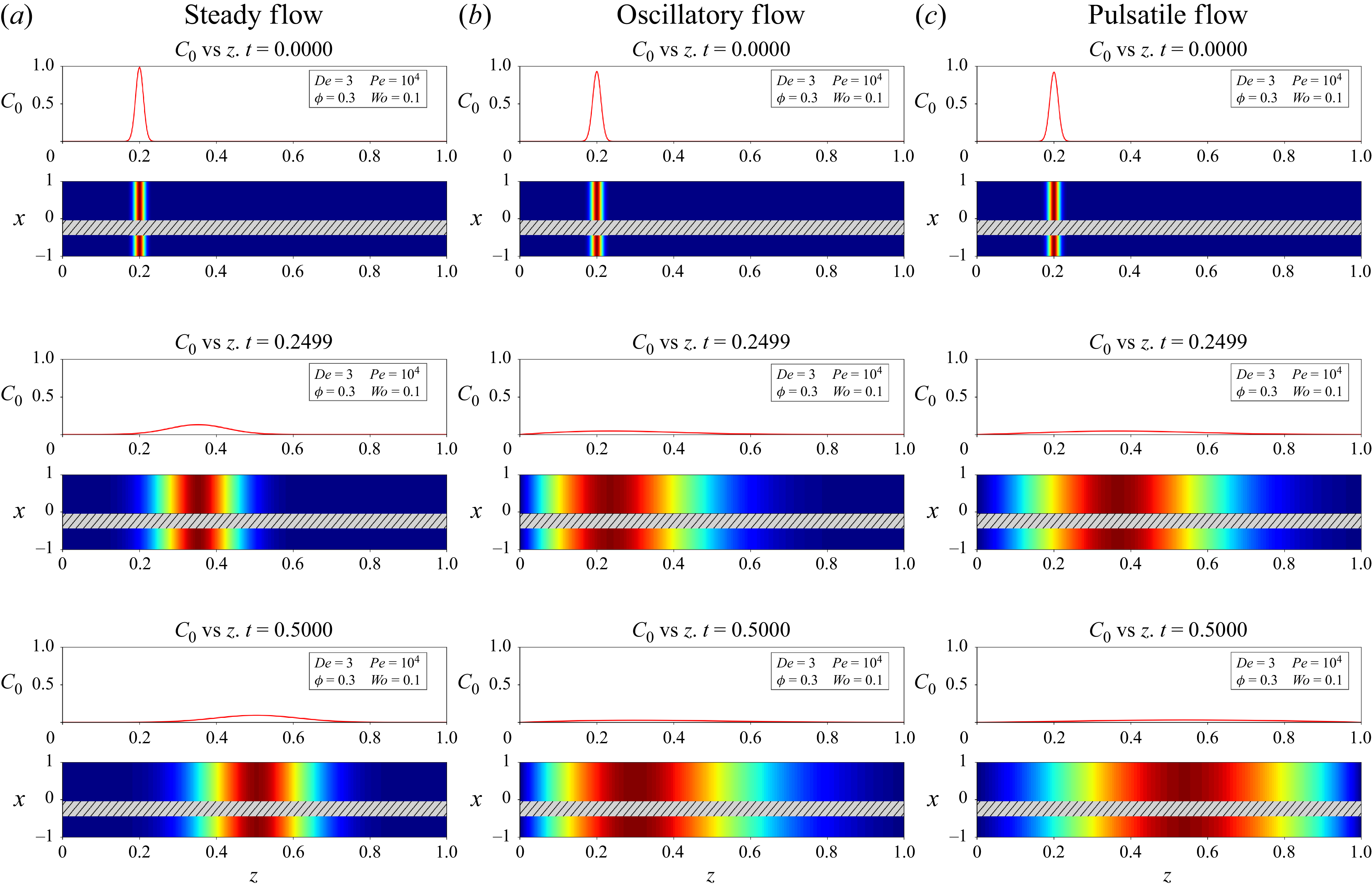
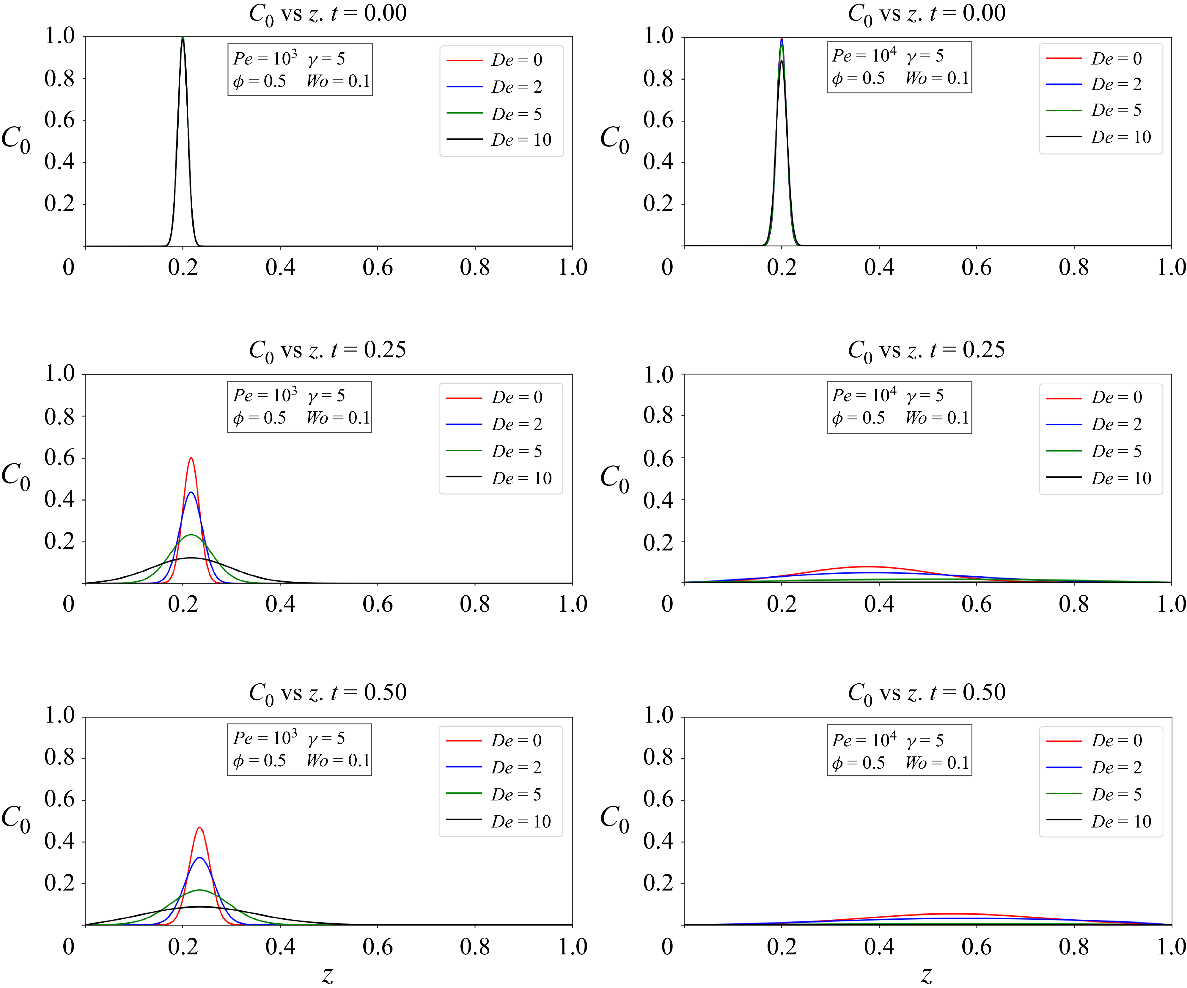
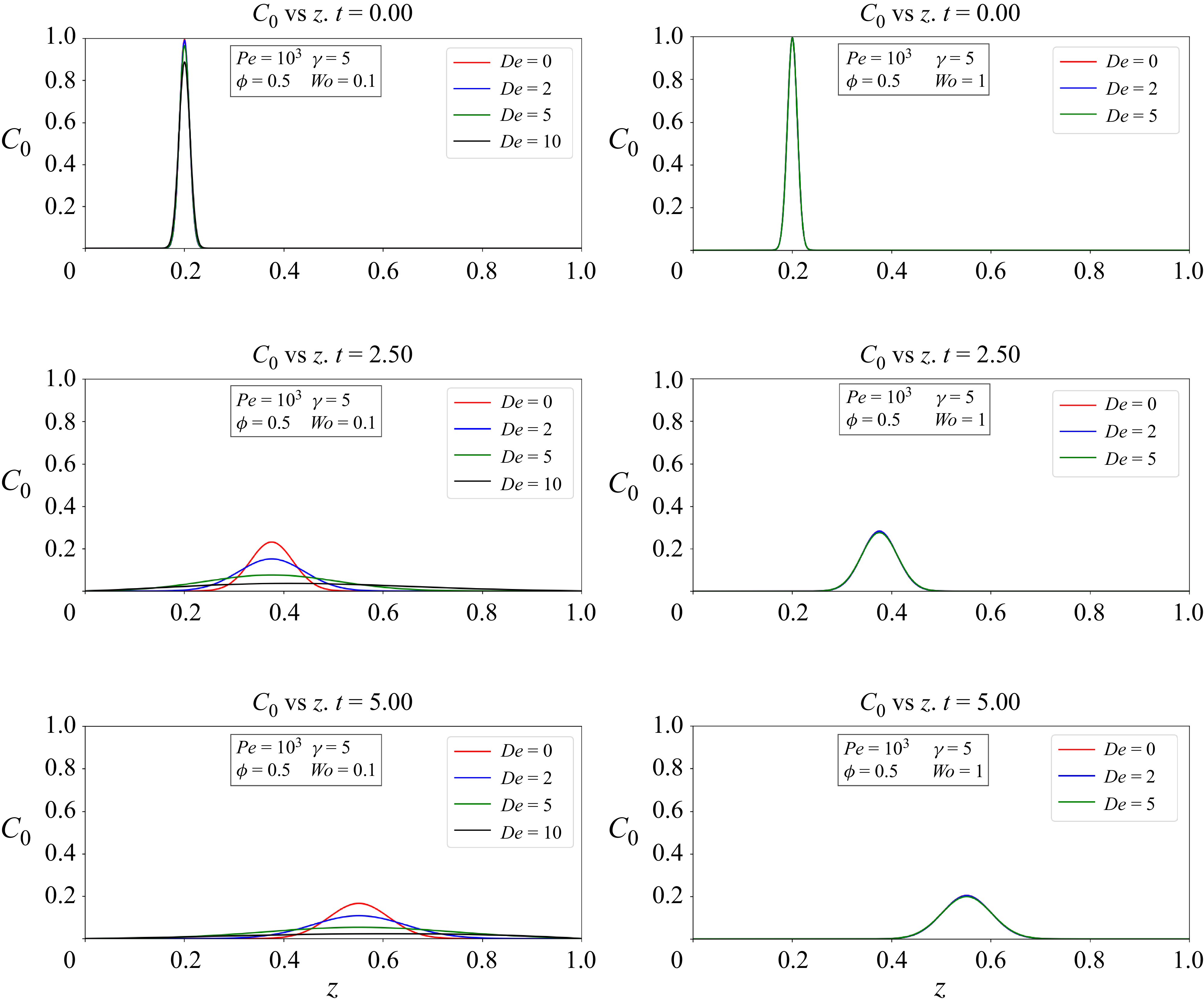
Figures 10, 11 and 12 contain selected frames at different dimensionless times from the animations available in the supplementary movies are available at https://doi.org/10.1017/jfm.2026.11286. Here, we have plotted the time evolution of the mean concentration along the channel. The plots of
 $C_{0}$
on the
 $z$
-axis are supported by contour plots illustrating the dispersion of the mean concentration in a two-dimensional representation of the annuli with the shaded section representing the inner cylinder.
Figure 10 shows that the eccentricity of the annuli improves the dispersion of the solute along the channel. These plots are an extension of the conclusions reported by Sankarasubramanian & Gill (Reference Sankarasubramanian and Gill1971) and Chu et al. (Reference Chu, Garoff, Tilton and Khair2020) for a Newtonian fluid for the mean concentration and in figure 4(c–h) it can be shown that this also applies to a viscoelastic fluid. An eccentric configuration contributes significantly to both convective and diffusive transports in the axial direction, resulting in rapid dispersion along this axis. With a dimensionless time of 0.5, the maximum concentration of the solute is approximately
 $0.1$
dimensionless units further in
 $z$
than with a concentric geometry. Moreover, the extent of the cloud of the solute in the axial dispersion is approximately twice that observed in the concentric case.
Figure 11 shows a significant improvement in the dispersion of the mean concentration of a fluid with
 ${\textit{De}} = 2$
. According to figure 8, however, an increase in
 ${\textit{Wo}}$
leads to a reduction in this enhancement.
Figure 12 shows that pulsatile flow generates the most significant dispersion along the channel. This is evident from the farthest-reaching concentration peak and the broader spreading of the concentration cloud. However, this enhancement in dispersion due to pulsatile flow is only observed at low frequencies. As the Womersley number increases, the plots in figure 12(c) begin to resemble those in figure 12(a). Additionally, an interesting observation from figure 12(b) is its consistency with classical studies on dispersion in oscillatory flows, which demonstrate that, even in the presence of a net zero flow, there is still a positive dispersion of the solute.
Equation (4.30) demonstrates that the Péclet number is crucial in determining the behaviour of mean concentration dispersion. An increase in the Péclet number enhances the combined effects of convective and diffusive transport. The plots in figure 13 support this analysis and align with the definition of the Péclet number. Specifically, at a lower Péclet number, diffusion dominates mass transport, and the rate of diffusive moment transport is slow, as shown in figure 13(a). In contrast, figure 13(b) illustrates the combined effects of both types of diffusion, resulting from a higher Péclet number, which significantly enhances mass transport along the channel.
To highlight the effect of the Womersley number on dispersion in viscoelastic fluids, simulations with different Deborah numbers are compared in figure 14. It can be observed that at low frequencies, the effective diffusion term in (4.30) increases significantly with the contribution of the oscillatory component to the effective dispersion coefficient. Consequently, the mean concentration spreads faster along the channel with increasing Deborah number compared with the Newtonian case, indicating that the fluid’s behaviour becomes more elastic. However, as the Womersley number increases, inertial forces dominate, and the effect of the relaxation time becomes insignificant. Therefore, the oscillatory dispersion coefficient in (4.30) gradually vanishes, and the equation reduces to its steady-state form, in which the viscoelastic effects are negligible.
Influence of Womersley number on mean concentration in a pulsatile flow for viscoelastic fluids. Considering
 $\epsilon = 0.001$
,
 $g = 1$
and
 ${Sc} = 10^{3}$
. An animation of this figure is provided in Supplementary Movie 5.

6. Conclusions
In this work, Taylor’s dispersion theory was applied using a semi-analytical method based on homogenization theory to numerically solve various perturbation problems. These problems were tackled using finite-difference methods, specifically the ADI scheme and the Crank–Nicolson method. The study analyses the dispersion of a neutral solute in a channel with an eccentric annulus configuration, where the flow can be steady, oscillatory or pulsatile. The fluid’s rheology is modelled with the Maxwell model. These flow types and fluid characteristics were selected due to the nature of biological fluids and their associated flow dynamics, where Taylor dispersion processes can occur.
The effective dispersion coefficient, which is composed of the steady and oscillatory dispersion coefficients, was determined in conjunction with a macrotransport equation that describes the behaviour of the mean concentration on a long-time scale. In this equation, an effective diffusion term for the concentration is derived, which includes the combined effect of transverse diffusion and convection due to the velocity profile.
Previous works have concluded that eccentricity and an increment in the annular section enhance both the velocity profile and the effective dispersion coefficient. Here, we demonstrate that this relationship also applies to viscoelastic fluids. Furthermore, the effective dispersion is significantly improved as
 ${\textit{De}}$
increases. The combined effects of eccentricity, viscoelasticity and pulsatile flow, which more accurately represent physiological conditions, lead to a markedly greater dispersion compared with the case of a concentric geometry with a Newtonian fluid and steady flow. Based on the results obtained, we have made further interesting observations.
-
(i) The Womersley number is the most important parameter for controlling enhancement in both Newtonian and non-Newtonian fluids. At low frequencies, the magnitude of the oscillatory velocity increases only in viscoelastic fluids, while it decreases in Newtonian ones. In this frequency range, a phenomenon known as viscoelastic resonance occurs, as previously reported by other authors, and is characterised by the appearance of resonant frequencies where the velocity magnitude is enhanced. Specifically, for viscoelastic fluids in eccentric configurations, if the Deborah number, the eccentricity and/or the gap width are increased, the velocity magnitude also increases at the first and most significant resonant frequency, which is additionally shifted to lower values of the Womersley number.
-
(ii) The viscoelastic effect at high frequencies is negligible due to the small contribution of the oscillatory dispersion coefficient.
-
(iii) As far as the mean concentration is concerned, the pulsatile flow produces a greater dispersion than the steady and oscillatory regimes. In addition, oscillatory flow always generates a positive dispersion of the solute, which is enhanced by the eccentricity and the viscoelastic properties of the fluid.
-
(iv) By definition, the Péclet number is related to the competition between convective and diffusive transport. When this parameter is appropriately selected, both mechanisms make significant contributions to the mean concentration distribution along the channel. In the macrotransport equation,
${\textit{Pe}}$
has a direct effect on both the convective and effective diffusion terms. Consequently, for large Péclet numbers, the cloud solute spreads more easily along the channel due to the dominance of convective transport.

In future research, additional features could be incorporated, such as wall reactions, slip boundary conditions and the consideration of oscillatory flows with more than one frequency to provide a more accurate representation of specific physical phenomena. Furthermore, it would be valuable to attempt an analytical approximation of this problem for small eccentricities using the domain perturbation method (Leal Reference Leal2007). In addition, a promising area to explore is the analysis of the dispersion process in annular, concentric and eccentric tubes with flexible walls.
Power-law relationship between
 $\mathscr{D}_{\textit{eff}}$
and (
 $\gamma - 1$
).

Supplementary movies
Supplementary movies are available at https://doi.org/10.1017/jfm.2026.11286.
Acknowledgements
G. Covarrubias acknowledges the support of the Secretaría de Ciencia, Humanidades, Tecnología e Innovación (SECIHTI) and the Instituto Politécnico Nacional (IPN). J. Arcos and O. Bautista acknowledge the Red de Energía and the Red de Nanociencia y Micro-nanotecnología for their support.
Funding
G. Covarrubias received financial support through a PhD fellowship from the Secretaría de Ciencia, Humanidades, Tecnología e Innovación (SECIHTI) and the Instituto Politécnico Nacional (IPN). J. Arcos and O. Bautista acknowledge financial support from the Secretaría de Investigación y Posgrado, Instituto Politécnico Nacional of México, through Research Grants 20251090 and 20250739, respectively.
Declaration of interests
The authors report no conflicts of interest.
Appendix A.
This Appendix presents the various expressions we have used to validate our numerical solution. The analytical expression for the steady velocity profile in an eccentric annulus provided by Snyder & Goldstein (Reference Snyder and Goldstein1965) is as follows:
 \begin{equation} v = F + E \eta - \frac {\coth \eta }{2} + \sum ^{\infty }_{n = 1} \left \{\left [A_{n}e^{n \eta } + \left (B_{n} - \coth \eta \right )e^{-n\eta } \right ]\cos n\xi \right \} ,\end{equation}
where
 \begin{align} F &= \frac {\alpha \coth \beta - \beta \coth \alpha }{2 \left (\alpha - \beta \right )},\\[-12pt]\nonumber\end{align}
 \begin{align} E &= \frac {\coth \alpha - \coth \beta }{2 \left (\alpha - \beta \right )},\\[-12pt]\nonumber\end{align}
 \begin{align} A_{n} &= \frac {\coth \alpha - \coth \beta }{e^{2n\alpha } - e^{2n\beta }},\\[-12pt]\nonumber\end{align}
 \begin{align} B_{n} &= \frac {e^{2n\alpha }\coth \beta -e^{2n\beta } \coth \alpha }{e^{2n\alpha } - e^{2n\beta }}. \end{align}
In the context of our physical variables, the definition of the dimensionless velocity is
 \begin{equation} v = \dfrac {\tilde {w}}{\dfrac{\tilde {G}_0 \tilde {a}^{2}}{\tilde {\mu }}}. \end{equation}
To validate the function
 $H$
and the steady dispersion coefficient
 $\mathscr{D}_{s}$
, we have solved the following equations provided by Chu et al. (Reference Chu, Garoff, Tilton and Khair2020).
Momentum equation
 \begin{equation} \left (\frac {\zeta }{a} \right )^{2} \left (\frac {\partial ^2 S}{\partial \xi ^2} + \frac {\partial ^2 S}{\partial \eta ^2}\right ) + \left [\left (1 + i \right )\sqrt {\frac {\omega }{2 {Sc}}}\right ]^{2} S = -\epsilon ^{2}, \end{equation}
where, the dimensionless angular frequency is
 \begin{equation} \omega = \frac {\tilde {\omega }}{\dfrac{\tilde {D}}{\tilde {r}^{2}_{2}}}. \end{equation}
In the context of our physical variables, the definition of the dimensionless velocity is
 \begin{equation} S = \dfrac {\tilde {w}}{\dfrac{\tilde {G}_0 \tilde {L}^{2}}{\tilde {\mu }}}. \end{equation}
If
 $\omega$
is zero,
 $S$
corresponds to our steady velocity profile
 $W_s$
. If
 $\omega$
is a finite value, S corresponds to our proposed function
 $H$
, for Newtonian fluids only. For the steady canonic cell equation, where
 $A$
corresponds to our
 $B_{s}$
 \begin{equation} \left (\frac {\zeta }{a} \right )^{2} \left (\frac {\partial ^2 A}{\partial \xi ^2} + \frac {\partial ^2 A}{\partial \eta ^2}\right ) = \bar {s} - \left \langle \bar {s}\right \rangle\! , \end{equation}
where
 $\bar {s}$
is the time average of the steady velocity profile, while
 $\langle \bar {s} \rangle$
is the area average of the time average of the steady velocity profile.