

1. Introduction
Owing to heightened environmental regulations, there has been a move towards using lean premixed combustors (LPCs) for their ability to operate at lower temperatures in a low  $\mathsf {NO}_{\mathsf {x}}$ regime (Correa Reference Correa1998). Whilst there are many health and environmental advantages to avoiding the production of
 $\mathsf {NO}_{\mathsf {x}}$, which is a lung irritant and can cause acid rain and depletion of the Ozone layer (Mahashabde et al. Reference Mahashabde2011), LPCs present many practical issues, including their susceptibility towards thermoacoustic instability (Culick Reference Culick1996; Lieuwen & Yang Reference Lieuwen and Yang2005).
Thermoacoustic instability arises owing to a feedback mechanism between acoustic waves and unsteady heat release. Unsteady heat release produces acoustic fluctuations which in turn interact with the flame causing more unsteady heat release. If these acoustic fluctuations are in phase with the unsteady heat release, this causes energy to be added to the system, which can lead to instability. This mechanism was first described by Rayleigh (Reference Rayleigh1878) who summarised it by a simple, but effective, integral criterion. Even though Rayleigh's criterion for instability is mathematically simple, the fact that this mechanism is extremely sensitive to the parameters of the system (Juniper & Sujith Reference Juniper and Sujith2018) means that the accurate prediction of thermoacoustic instabilities is a difficult task, which leads to many combustion systems being built vulnerable to these instabilities.
As these instabilities can cause material fatigue and lifetime reduction for these systems, it is critical to develop control strategies to either suppress, or remove entirely, these instabilities (Candel Reference Candel2002). These control strategies can fall into two categories: active (McManus, Poinsot & Candel Reference McManus, Poinsot and Candel1993; Zhao et al. Reference Zhao, Lu, Zhao, Li, Wang and Liu2018) and passive (Zhao & Li Reference Zhao and Li2015). Examples of passive control include the addition of Helmholtz resonators to provide acoustic damping (Dupère & Dowling Reference Dupère and Dowling2005). Alternatively, active control uses actuation devices such as loudspeakers to provide an additional source of acoustic waves (Dowling & Morgans Reference Dowling and Morgans2005). Furthermore, the aforementioned sensitivity of these systems to parameters has made adjoint methods an attractive tool in designing these controls (Magri Reference Magri2019), for example, in optimising the shape and placement of Helmholtz resonators (Yang et al. Reference Yang, Sogaro, Morgans and Schmid2019) or for discovering the optimal feedback mechanism for suppressing the growth rate of instabilities (Magri & Juniper Reference Magri and Juniper2013). Of particular relevance to our study is the open-loop control via harmonic forcing of the thermoacoustic system and adjoint design methods based on Floquet theory (Magri Reference Magri2019).
By introducing harmonic forcing, the phase relationship between the unsteady heat release and pressure perturbations can be disrupted leading to a decrease in the self-sustained limit cycle oscillations (Kashinath, Li & Juniper Reference Kashinath, Li and Juniper2018; Mondal, Pawar & Sujith Reference Mondal, Pawar and Sujith2019; Roy et al. Reference Roy, Mondal, Pawar and Sujith2020). Depending on the value of the forcing frequency in relation to the natural frequency of the limit cycle, this decrease can be split into two cases. Synchronous quenching occurs if the forcing is close to the natural frequency and although the self-excited oscillations are suppressed, the system synchronises to the forcing frequency, which causes a resonant amplification. However, if the forcing frequency is farther away from the natural frequency, then a reduction in the self-excited oscillations can occur without resonant amplification. Therefore, understanding a priori the synchronisation properties of the system is of upmost importance to determine good candidate frequencies and forcing shapes that result in synchronisation away from resonant frequencies. The aim of this study is to apply phase-reduction analysis to thermoacoustic systems, an adjoint Floquet-based method, which will allow the synchronisation characteristics of the system to be obtained efficiently from numerical simulations. Furthermore, we will showcase the usefulness of this information in the design of open-loop control strategies via harmonic forcing.
Phase-reduction analysis is a technique that has been widely used for studying the dynamics of synchronisation in biological systems (Kuramoto Reference Kuramoto1984; Pikovsky, Rosenblum & Kurths Reference Pikovsky, Rosenblum and Kurths2003; Ermentrout & Terman Reference Ermentrout and Terman2010; Boccaletti et al. Reference Boccaletti, Pisarchik, del Genio and Amann2018). It is only relatively recently that phase reduction has been introduced to the fluids community (Kawamura & Nakao Reference Kawamura and Nakao2015; Taira & Nakao Reference Taira and Nakao2018; Iima Reference Iima2019; Khodkar & Taira Reference Khodkar and Taira2020; Khodkar, Klamo & Taira Reference Khodkar, Klamo and Taira2021; Loe et al. Reference Loe, Nakao, Jimbo and Kotani2021; Nair et al. Reference Nair, Taira, Brunton and Brunton2021). In essence, phase reduction allows the linear phase dynamics of a stable periodic system to be represented by a simple scalar ordinary differential equation (ODE) for the phase. This ODE is characterised by the phase sensitivity function which encodes properties of how external forcing affects the phase. Obtaining the phase sensitivity function therefore allows for the efficient determination of the synchronisation properties of the underlying system, which in the present study is focused on thermoacoustic systems. In what follows, § 2 outlines the Rijke tube model, § 3 lays out the mathematics of phase-reduction analysis, the numerics are described in § 4, the results are presented in § 5 and finally, the conclusions are offered in § 6. Appendix A contains further mathematical details of the method, as well as solidifying the link between phase-sensitivity analysis and Floquet theory (Floquet Reference Floquet1883) for delay differential equations (Simmendinger, Wunderlin & Pelster Reference Simmendinger, Wunderlin and Pelster1999).
2. The Rijke tube: an example thermoacoustic system
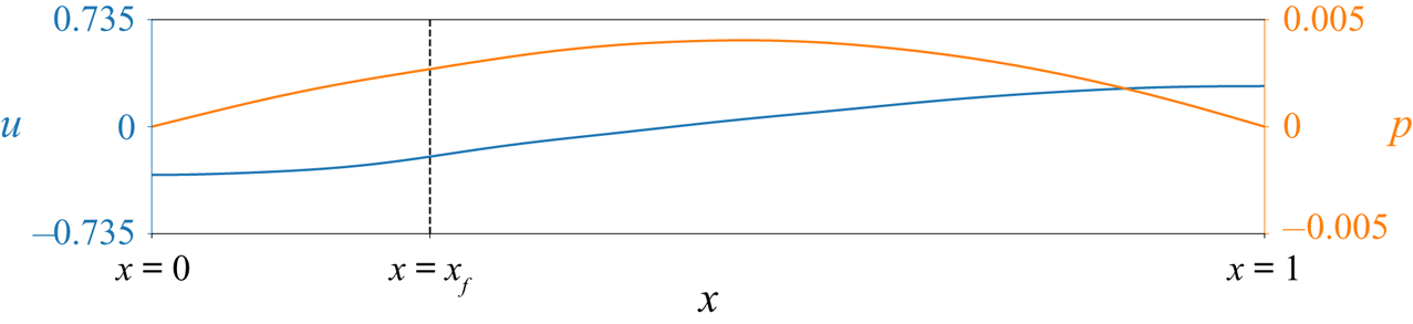
A Rijke tube (Rijke Reference Rijke1859) is a relatively simple set-up that exhibits a rich range of dynamics with thermoacoustic instability. We show the basic set-up in figure 1 and model the system as a one-dimensional flow in a pipe. The left side of the pipe is aligned with  $x=0$, with the pipe having a non-dimensional unit length. A heat source is placed at
 $x=x_f$, and is modelled as a thin wire using a modified version (Heckl Reference Heckl1990) of King's law (King Reference King1914).
Rijke tube set-up with example velocity and pressure profiles.

Following the derivation in Sayadi et al. (Reference Sayadi, Le Chenadec, Schmid, Richecoeur and Massot2014), the non-dimensional governing equations for this system are provided by
 $$\begin{gather} \frac{\partial u}{\partial t}+(\gamma\textit{Ma})^{{-}1}\frac{\partial p}{\partial x}= 0, \end{gather}$$
 $$\begin{gather}\frac{\partial p}{\partial t}+(\gamma\textit{Ma})\frac{\partial u}{\partial x}+\xi*p=\gamma\textit{Ma}Q+\epsilon f_p^+, \end{gather}$$
for the velocity  $u$ and the pressure
 $p$, which form our state space
 $\boldsymbol {y}=(u,p)^\textrm {T}$. Following the work of Mondal et al. (Reference Mondal, Pawar and Sujith2019), a weak external pressure forcing
 $f_p^+$ with amplitude
 $\epsilon \ll 1$ is added to the pressure field. The governing equations hold two non-dimensional parameters of Mach number
 $Ma$ and the specific heat ratio
 $\gamma$. The damping for wavenumber
 $j$ is given via a convolution
 $*$ in terms of damping coefficients
 $c_1$ and
 $c_2$ as
 $\xi _j=c_1j^2+c_2\sqrt {j}$. We see that the only nonlinearity that enters the equation is through the heat release rate term,
 \begin{equation}
Q=Q_f(t-\tau)\delta(x-x_f)=\frac{K}{2}\left(\sqrt{|1/3+u_f(t-\tau)|}-\sqrt{1/3}\right)\delta(x-x_f),
\end{equation}
which is localised to the flame location  $x_f$, using a Dirac delta function
 $\delta$, with a time-dependent amplitude
 $Q_f$ that depends on the velocity at the flame
 $u_f$, flame time delay
 $\tau$ and the heater strength
 $K$. This system is a delay partial differential equation (DPDE) owing to the lag introduced through the heating term. Therefore, the initial condition for this equation must be specified for
 $t\in [t_0-\tau,t_0]$. We apply open boundaries at the pipe ends, which correspond to homogeneous Dirichlet and Neumann conditions for
 $p$ and
 $u$, respectively.
For a sufficiently large  $K$, the fixed point
 $(u,p)=(0,0)$ is unstable and, for all parameter regimes considered in this study, nonlinear saturation of this instability yields a self-sustained limit cycle with period
 $T$. As we are dealing with a DPDE whose solution must be known over
 $[t-\tau,t]$ to propagate the solution forward, the limit cycle is actually defined up to
 $\tau$ time-units previously. To make this dependence on the history of the system clear, we now introduce the following notation (Hale Reference Hale1977) (see Appendix A for further details). In what follows, we consider the discretised system and write the state-equation as the delay differential equation (DDE)
 \begin{equation} \dot{\boldsymbol{y}}=\boldsymbol{f}(t,\boldsymbol{y}(t))+\boldsymbol{g}(t-\tau,\boldsymbol{y}(t-\tau))+\epsilon \boldsymbol{h}(t),\end{equation}
with  $\boldsymbol {f}$,
 $\boldsymbol {g}$ and
 $\boldsymbol {h}$ arising from the discretisation of (2.2). We write a solution to this equation in the form
 $\boldsymbol {y}_t(\phi )=\boldsymbol {y}(t+\phi )$, where
 $\phi \in [-\tau,0]$. In particular, we can express our limit cycle, a periodic solution in the absence of forcing (
 $\epsilon =0$), as
 $\boldsymbol {y}^{LC}_t(\phi )$, where
 $\boldsymbol {y}^{LC}_{t+T}(\phi )=\boldsymbol {y}^{LC}_{t}(\phi )$.
3. Phase-reduction analysis
For a given limit cycle, we can introduce the concept of phase through a two-part definition. First, we associate the phase  $\theta$ with states
 $\boldsymbol {y}^{LC}_t(\phi )$ on the limit cycle via
 $\theta =2{\rm \pi} t/T\; \textrm {mod}\; 2{\rm \pi}$. Hence, the phase
 $\theta \in [0,2{\rm \pi} ]$ is a scalar variable that represents the limit cycle. Second, we extend the phase definition to states in the vicinity of our limit cycle by restricting ourselves to limit cycles that are asymptotically stable. This means that if
 $\boldsymbol {y}_t(\phi )$ is a state not necessarily on the limit cycle, then there exists a state on the limit cycle
 $\boldsymbol {y}^{LC}_{t+\alpha }(\phi )$ such that
 $\|\boldsymbol {y}_t(\phi )-\boldsymbol {y}^{LC}_{t+\alpha }(\phi ))\|\rightarrow 0$ as
 $t\rightarrow \infty$. We can then say that the phase of
 $\boldsymbol {y}_t(\phi )$ is the same as the point in time it asymptotically tends to and therefore
 $\varTheta (\boldsymbol {y}_t(\phi ))=\varTheta (\boldsymbol {y}^{LC}_{t+\alpha }(\phi ))$, where the phase function
 $\varTheta$ is defined such that
 $\varTheta (\boldsymbol {y}_t(\phi ))=\theta$. While the phase is directly related to the time variable in this problem, phase can, in general, be related to sensor measurements (Nakao Reference Nakao2016; Taira & Nakao Reference Taira and Nakao2018). It is also worth noting that whilst alternative definitions of phase can be introduced, the motivation behind our definition is that it will allow us to study the synchronisation properties of the limit cycle using linear theory.
For states on the limit cycle, the phase  $\theta$ satisfies
 $\dot {\theta }=\omega _n=2{\rm \pi} /T$, where
 $\omega _n$ is the angular frequency of the limit cycle. However, in the presence of a small external forcing, the phase equation becomes (Kotani et al. Reference Kotani, Yamaguchi, Ogawa, Jimbo, Nakao and Ermentrout2012; Novičenko & Pyragas Reference Novičenko and Pyragas2012)
 \begin{equation} \dot{\theta}=\omega_n+\epsilon \boldsymbol{Z}(\theta)^\textrm{T}\boldsymbol{h}(t)+{O}(\epsilon^2). \end{equation}
The function  $\boldsymbol {Z}(\theta )$ is the phase-sensitivity function and allows us to assess the influence of a perturbation
 $\boldsymbol {h}(t)$ on the phase dynamics. To determine this phase-sensitivity function, two main methods can be employed. The first of which is to perturb the equation for a range of values of
 $\theta$, building up the function one point at a time (Taira & Nakao Reference Taira and Nakao2018). A second approach, which we consider, finds
 $\boldsymbol {Z}$ as the solution to an adjoint problem (Kotani et al. Reference Kotani, Yamaguchi, Ogawa, Jimbo, Nakao and Ermentrout2012; Novičenko & Pyragas Reference Novičenko and Pyragas2012).
For the latter approach, we begin by linearising the unperturbed governing equations (2.4) about the limit cycle  $\boldsymbol {y}^{LC}_t(\phi )$ providing the linear DDE
 \begin{equation} \dot{\boldsymbol{y}}'=\boldsymbol{\mathsf{A}}_1(t)\boldsymbol{y}'(t)+\boldsymbol{\mathsf{A}}_2(t)\boldsymbol{y}'(t-\tau). \end{equation}
This equation describes the dynamics of a small perturbation  $\boldsymbol {y}'$ about the limit cycle. Here, the matrices
 $\boldsymbol{\mathsf{A}}_1$ and
 $\boldsymbol{\mathsf{A}}_2$ are the Jacobians
 $\boldsymbol{\mathsf{A}}_1(t)=\nabla _{\boldsymbol {y}} \boldsymbol {f}( \boldsymbol {y})|_{\boldsymbol {y}=\boldsymbol {y}_t(0)}$ and
 $\boldsymbol{\mathsf{A}}_2(t)=\nabla _{\boldsymbol {y}} \boldsymbol {g}(\boldsymbol {y})|_{\boldsymbol {y}=\boldsymbol {y}_{t}(-\tau )}$, respectively. As discussed more extensively in Appendix A, we must first define a bilinear form to introduce the adjoint for a DDE. For the present DDE, the appropriate bilinear form (Kotani et al. Reference Kotani, Yamaguchi, Ogawa, Jimbo, Nakao and Ermentrout2012; Novičenko & Pyragas Reference Novičenko and Pyragas2012) is
 \begin{equation} \langle\boldsymbol{a}(t),\boldsymbol{b}(t)\rangle\equiv\boldsymbol{a}(t)^\textrm{T}\boldsymbol{b}(t)+\int_{-\tau}^0\boldsymbol{a}(t+\tau+\xi)^\textrm{T}\boldsymbol{\mathsf{A}}_2(t+\tau+\xi)\boldsymbol{b}(t+\xi)\,\textrm{d}\xi. \end{equation}
Using this bilinear form, the adjoint can be found (see Appendix A) to satisfy the adjoint equation
 \begin{equation} \dot{\boldsymbol{y}}^{\dagger}{=}{-}\boldsymbol{\mathsf{A}}_1^\textrm{T}(t)\boldsymbol{y}^{\dagger}(t)-\boldsymbol{\mathsf{A}}_2^\textrm{T}(t+\tau)\boldsymbol{y}^{\dagger}(t+\tau). \end{equation}
With the linear equation (3.2) and its adjoint (3.4), we can find the phase-sensitivity function via the link between a phase shift and Floquet theory, which governs the stability of the limit cycle. As we have assumed that the limit cycle is stable, all the Floquet exponents are inside the unit circle, except for one which provides the phase shift. Indeed, for an autonomous system, there is always one neutral Floquet exponent, which has the eigenvector  $\dot {\boldsymbol {y}}^{LC}_t(\phi )$.
The Floquet exponents for the adjoint system (3.4) are the negative complex conjugates of the direct case. This means that by solving equation (3.4) backwards in time, the system is stable and has one neutral Floquet exponent with the corresponding eigenvector  $\boldsymbol {y}^{\dagger} _t(\phi )$. Normalising this eigenvector such that
 $\langle \boldsymbol {y}^{\dagger} _t(\phi ), \dot {\boldsymbol {y}}^{LC}_t(\phi ) \rangle =\omega _n$ yields the phase-sensitivity function via
 $\boldsymbol {Z}(\theta ) = \boldsymbol {y}^{\dagger} _{t=\theta /\omega _n}(0)$ (see Appendix A for details). In practice, we can find the adjoint eigenvector by integrating (3.4) back in time from an arbitrary initial condition to obtain the ‘adjoint limit-cycle’, which, given a sufficiently long time horizon, converges to the neutral Floquet solution.
Using the phase-sensitivity function, the phase-coupling function can be determined. We consider the general case of  $m:n$ phase locking, which means that for
 $m$ periods of the external forcing, the system completes
 $n$ cycles. By introducing the phase difference
 $\Delta \theta (t)=\theta (t)-(n/m) \omega _f t$, and assuming that
 $\Delta \theta (t)$ is slowly varying, it can be shown (see Khodkar & Taira Reference Khodkar and Taira2020 for example) that synchronisation will occur if
 \begin{equation} \epsilon \min_{\Delta\theta} \varGamma_{m,n}(\Delta\theta) <(n/m)\omega_f-\omega_n< \epsilon \max_{\Delta\theta} \varGamma_{m,n}(\Delta\theta), \end{equation}
where
 \begin{equation} \varGamma_{m,n}(\Delta\theta) \equiv \frac{1}{m T_f}\int_{t_0}^{t_0+m T_f} \boldsymbol{Z}(\Delta\theta(t)+(n/m) \omega_f s)^\textrm{T}\boldsymbol{h}(s) \,\textrm{d}s, \end{equation}
is the phase-coupling function and  $T_f$ is the period of the external forcing. This inequality gives a region of synchronisation over the space of forcing angular frequency
 $\omega _f$ and forcing amplitude
 $\epsilon$, known as an Arnold tongue, in which
 $m:n$ frequency locking is possible.
4. Numerical implementation
To numerically solve the governing equations (2.2), we consider the Galerkin projection approach of Balasubramanian & Sujith (Reference Balasubramanian and Sujith2008). With expansions
 $$\begin{gather} u = \sum_{j=1}^N \eta_j(t)\cos(j{\rm \pi} x), \end{gather}$$
 $$\begin{gather}p ={-}\sum_{j=1}^N \left(\frac{\dot{\eta_j}(t)\gamma\textit{Ma}}{j{\rm \pi}}\right)\sin(j{\rm \pi} x), \end{gather}$$
 $$\begin{gather}f_{p}^+{=} \sum_{j=1}^N f_{pj}^+\sin(j{\rm \pi} x), \end{gather}$$
we automatically satisfy the boundary conditions and reduce the full DPDE to a DDE for the coefficients  $\eta _j$ and
 $\dot {\eta _j}$. The heat release terms become
 $$\begin{gather} u_f=\sum_{j=1}^N\eta_j(t-\tau)\cos(j{\rm \pi} x_f), \end{gather}$$
 $$\begin{gather}\dot{q}_j=j{\rm \pi} K(\sqrt{|1/3+u_f|}-\sqrt{1/3})\sin(j{\rm \pi} x_f), \end{gather}$$
and we can write the system (2.2) as
 \begin{equation} \ddot{\eta}_j+(j{\rm \pi})^2\eta_j+\xi_j\dot{\eta}_j={-}\dot{q}_j-\frac{j{\rm \pi}\epsilon}{\gamma\textit{Ma}} f^+_{pj}.\end{equation}
This equation can be recast to the first-order DDE
 \begin{equation} \frac{\textrm{d}}{\textrm{d}t}\begin{pmatrix} \boldsymbol{\eta}(t)\\ \dot{\boldsymbol{\eta}}(t) \end{pmatrix}=\begin{pmatrix} \boldsymbol{\mathsf{0}} & \boldsymbol{\mathsf{I}} \\ \boldsymbol{\mathsf{W}} & \boldsymbol{\mathsf{D}} \\ \end{pmatrix} \begin{pmatrix} \boldsymbol{\eta}(t)\\ \dot{\boldsymbol{\eta}}(t) \end{pmatrix} -\begin{pmatrix} \boldsymbol{0}\\ \dot{\boldsymbol{q}}(\boldsymbol{\eta(t-\tau)}) \end{pmatrix}-\epsilon \begin{pmatrix} \boldsymbol{0}\\ \,\boldsymbol{f}^+_{p} \end{pmatrix}, \end{equation}
where
 \begin{equation} {\boldsymbol{\eta}}=(\eta_1,\ldots,\eta_N)^\textrm{T}, \quad \boldsymbol{f}_p=({\rm \pi}/(\gamma\textit{Ma})f_{p1}\ldots,N{\rm \pi}/(\gamma\textit{Ma})f_{pN})^\textrm{T}, \end{equation}
and diagonal matrices  $\boldsymbol{\mathsf{W}}$ and
 $\boldsymbol{\mathsf{D}}$ have entries
 $\boldsymbol{\mathsf{W}}_{jj}=-(j{\rm \pi} )^2$ and
 $\boldsymbol{\mathsf{D}}_{jj}=-\xi _j$, respectively.
It is important to note that the size of  $\epsilon$ does not affect the phase-sensitivity function
 $\boldsymbol {Z}$ as this is determined through a linear formulation. However, when the phase-sensitivity function is used to find the bounds of synchronisation via (3.5), we are in effect using a first-order Taylor expansion in
 $\epsilon$ in which
 $\boldsymbol {Z}$ is the linear term. Therefore, the size of
 $\epsilon$ can affect the synchronisation region. Indeed,
 $\epsilon$ is the amplitude of the external forcing and it is useful to have a physical measure of how large this amplitude is. To this end, we introduce the total non-dimensional acoustic energy per unit volume of the system (Juniper Reference Juniper2011)
 \begin{equation} E=\frac{1}{2}\left[u^2+\frac{p^2}{(\gamma\textit{Ma})^2}\right] =\frac{1}{2}\sum_{j=1}^N\eta_{j}^2+\frac{1}{2}\sum_{j=1}^N\left(\frac{\dot{\eta}_{j}}{\,j{\rm \pi}}\right)^2. \end{equation}
This energy measure allows us to quantify the size of  $\epsilon$. In other words, we assess the magnitude of the added perturbation.
To obtain the linearised and adjoint equations, we cast the Galerkin model (4.7) in the form of a DDE (2.4). Here, we have
 \begin{equation} \boldsymbol{\mathsf{A}}_1=\begin{pmatrix} \boldsymbol{\mathsf{0}} & \boldsymbol{\mathsf{I}} \\ \boldsymbol{\mathsf{W}} & \boldsymbol{\mathsf{D}} \\ \end{pmatrix}, \quad \boldsymbol{\mathsf{A}}_2=\begin{pmatrix} \boldsymbol{\mathsf{0}} & \boldsymbol{\mathsf{0}} \\ \boldsymbol{\mathsf{B}} & \boldsymbol{\mathsf{0}} \\ \end{pmatrix}, \end{equation}
in our linearised equation (3.2), where
 \begin{equation} (\boldsymbol{\mathsf{B}})_{ij}(t)={-}\frac{i{\rm \pi} K\sin(i{\rm \pi} x_f)\,\text{sgn}(\frac{1}{3}+u_f(t-\tau))\cos(j{\rm \pi} x_f)}{2\sqrt{|\frac{1}{3}+u_f(t-\tau)|}}. \end{equation}
Our implementation, which is available (Skene & Taira Reference Skene and Taira2021), is based on the sixth-order DDE solver Vern6 (Verner Reference Verner2010) contained in the DifferentialEquations.jl package (Rackauckas & Nie Reference Rackauckas and Nie2017).
5. Results
Using the Galerkin expansion approach introduced above, we are able to systematically obtain the phase-sensitivity function for a given set of parameters. As our goal is not only to find the phase-sensitivity function, but also to assess the synchronisation dynamics with a view to open-loop forcing, we consider a range of values for the flame time delay  $\tau$, flame strength
 $K$ and flame location
 $x_f$. For all cases, we fix the number of Galerkin modes to
 $N=10$, which gives a reasonable compromise between obtaining higher-mode behaviour and keeping the computational run-time reasonable. We herein set the damping parameters to
 $c_1=0.1$ and
 $c_2=0.06$ and fix
 $Ma=0.005$ and
 $\gamma =1.4$. The neutral stability curves for the fixed point
 $(u,p)=(0,0)$ in
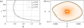
 $\tau -K$ space for different values of the flame location are shown in figure 2(a). In what follows, we only consider unstable cases as this will ensure that a limit cycle solution emerges. However, even in the stable regime, limit cycle solutions can be found, as in the study by Juniper (Reference Juniper2011), and the methods of this paper also carry over to these limit cycles, provided they are Floquet stable. It is also worth noting that Juniper (Reference Juniper2011) showed that owing to non-normality, a small perturbation can grow large enough to move the system away from its stable configuration, an effect which is not accounted for by our current analysis which is valid close to the limit cycle.
(a) Neutral curves for the stability of the fixed point  $(u,p)=(0,0)$. Highlighted with a blue cross are the parameters for our base case. (b) Plot of
 $u$ versus
 $p$ at
 $x=0.2$ for the direct solution. The transient behaviour is displayed in orange, with the limit cycle shown in blue.

We start by examining the case with  $K=0.72$,
 $x_f=0.25$ and
 $\tau =0.2$, following Mondal et al. (Reference Mondal, Pawar and Sujith2019). This baseline case is highlighted in figure 2(a) and is located just inside the unstable regime. To obtain the limit cycle, we solve (4.7) in the absence of external forcing and with a small random initial condition. For these parameters, the state
 $(u,p)=(0,0)$ is unstable, the perturbation grows and eventually saturates into a limit cycle. By starting at
 $t=-400$, we obtain a limit cycle (see figure 2b) free of transient effects by
 $t=0$, which is further integrated to
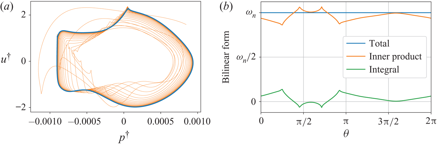
 $t=400$. This allows us to obtain the phase-sensitivity function by solving the adjoint equation backwards in time, starting from a random initial condition, from
 $t=400$ to
 $0$ (see figure 3a). We compute the phase-sensitivity function using the adjoint solution for
 $t\in [0,T]$ with
 $T = 1.93$, scaling with the normalisation specified in § 3. Whilst enabling us to fix the amplitude of the phase-sensitivity function, the inner product (3.3) also provides a good check of our adjoint solution. The inner product must be constant in time and consists of two parts; a dot product and an integral. Figure 3(b) confirms the value of the inner product being constant over one period, which verifies our adjoint solution.
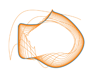
(a) Plot of  $u^{\dagger}$ versus
 $p^{\dagger}$ at
 $x=0.2$ for adjoint solution. Again, the transient behaviour is displayed in orange, with the limit cycle shown in blue. (b) The value of the bilinear form, as well as the breakdown into its inner product and integral contributions, over one period.

With the phase-sensitivity function determined, we can compute the phase-coupling function using (3.6). The forcing term is specified to be  $f_{pj}^+=-\gamma \textit {Ma}/(j{\rm \pi} )c\cos (\omega _f t)$ following Mondal et al. (Reference Mondal, Pawar and Sujith2019), with
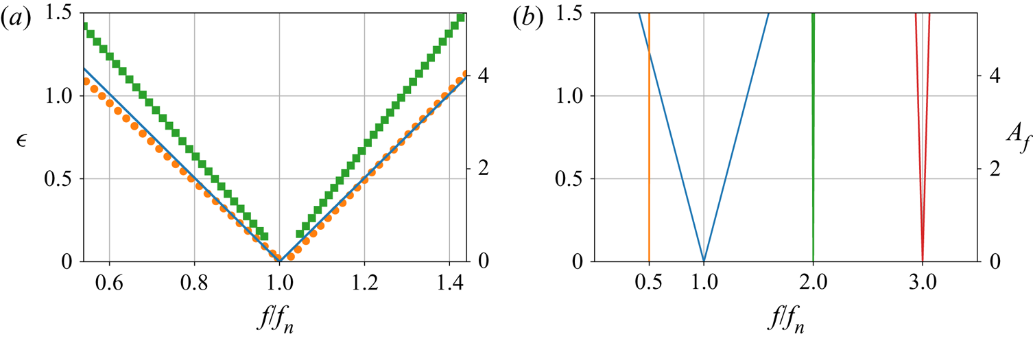
 $c$ chosen such that the forcing has a unit acoustic energy norm. The resulting Arnold tongue obtained from (3.5) is shown in figure 4(a). We have shown on the
 $y$-axis both the amplitude
 $\epsilon$ as well as
 $A_f$, which matches the amplitude displayed by Mondal et al. (Reference Mondal, Pawar and Sujith2019) owing to the different normalisations used. The ‘V’ shape shows the minimum amplitude of the forcing needed to obtain synchronisation at the different values of the frequency
 $f=\omega _f/(2{\rm \pi} )$, with synchronisation being possible inside the V-shaped region. We see that for frequencies equal to the natural frequency of the system
 $f_n$, synchronisation is always possible. However, as this frequency is increased or decreased, a greater forcing amplitude is needed.
(a) The Arnold tongue showing the regions where synchronisation is possible (blue line). Also displayed are the boundaries between phase trapping and phase drifting (orange circles), as well as phase locking and phase trapping (green squares) from Mondal et al. (Reference Mondal, Pawar and Sujith2019). (b) The Arnold tongues for the general cases of  $1:2$ (orange),
 $1:1$ (blue),
 $2:1$ (green) and
 $3:1$ (red) synchronisation.

Figure 4(a) shows that there is a good agreement between our obtained Arnold tongue and the one computed by Mondal et al. (Reference Mondal, Pawar and Sujith2019), which holds true even for large forcing amplitudes  $\epsilon$. The Arnold tongue calculated by Mondal et al. (Reference Mondal, Pawar and Sujith2019) required performing a series of nonlinear simulations at different forcing amplitudes to obtain, on a point-by-point basis, the resulting synchronisation behaviour. This means that the Arnold tongue they obtained includes nonlinear behaviour, such as phase trapping. In our case, we consider a linear analysis, which enables us to efficiently calculate the entire Arnold tongue with a single adjoint simulation. The differences can therefore be attributed to nonlinear effects. We also see that our Arnold tongue is symmetric. This symmetry has to occur when using a Galerkin model because both
 $u$ and
 $p$ have zero means. However, the experimentally obtained Arnold tongue (Mondal et al. Reference Mondal, Pawar and Sujith2019) has an asymmetry showing that synchronisation was easier for frequencies below the natural frequency. This is a direct consequence of their experimental set-up, which has a mean flow.
In addition to  $1:1$ synchronisation, figure 4(b) reveals the general case of
 $m:n$ phase locking predicted by the present analysis. The figure shows that
 $1:1$ synchronisation is the easiest to achieve, with
 $3:1$ frequency locking also being feasible, albeit over a narrower region. Perhaps most importantly, we see that for our system,
 $1:2$ synchronisation is impractical to attain. In the study of Mondal et al. (Reference Mondal, Pawar and Sujith2019), asynchronous quenching was achieved for frequencies lower than the natural frequency, a region in which
 $1:2$-type phase locking could occur. By obtaining figure 4(b), we can directly observe a priori the phase-locking behaviour in this region. This further emphasises the importance of obtaining the Arnold tongues in designing open-loop control strategies and highlights the capabilities of the phase-sensitivity method to efficiently find the synchronisation conditions.
The fact that the phase-sensitivity function is independent of the forcing function means that we can efficiently consider the optimal placement of the pressure forcing for the purpose of synchronisation. Identifying the optimal placement allows for designing effective open-loop control strategies to move the frequency of the limit cycle to a desired one for a particular system via synchronisation. This is similar to the approach of Khodkar & Taira (Reference Khodkar and Taira2020), where the optimal placement of actuators for synchronisation was considered in the case of vortex shedding behind a cylinder. To assess the ease (or difficulty) of achieving synchronisation, we consider synchronisability  $\mathcal {S} \equiv \max (\varGamma )-\min (\varGamma )$, which essentially represents the width of the Arnold tongue (Khodkar & Taira Reference Khodkar and Taira2020). Instead of a global pressure forcing, we now consider a pointwise placement of pressure actuation given by
 $f_p^+=\gamma \textit {Ma}\delta (x-x_p)\cos (\omega _f t)$, where
 $x_p$ is the actuator location along the Rijke tube. In terms of our Galerkin model, this corresponds to setting
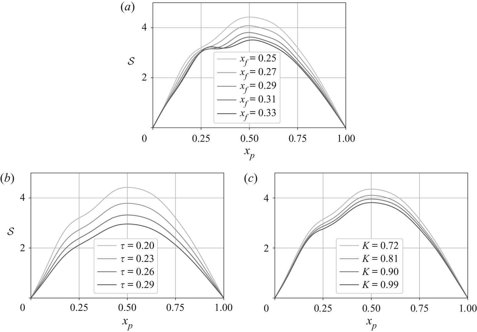
 $f_{pj}^+=2 \gamma \textit {Ma} \sin (j{\rm \pi} x_p)\cos (\omega _f t)$. We seek the synchronisability for a range of parameters, each requiring us to obtain a new phase-sensitivity function using the method described for our base case.
The synchronisability for varied  $x_p$ along the tube is shown in figure 5 for a wide range of parameters. In all cases, the maximum value of synchronisability occurs at
 $x_p=0.5$, i.e. half-way along the Rijke tube. The fact that the optimal location is at the tube mid-point could be attributed to the natural acoustic mode-shapes which all have a maximum at the midpoint. It also aligns with what was discovered for passive control via an adjoint analysis of the eigenvalue sensitivities (Magri & Juniper Reference Magri and Juniper2013), where a pressure based feedback forcing of the pressure equation was found to be maximal near the tube centre (approximately
 $x_p=0.58$). The difference between their location and ours could arise from the choice of linearisation. Namely, the fact that ours is around the limit cycle whereas theirs is around a fixed point. This is an important consideration because Juniper (Reference Juniper2011) shows that there are multiple stable limit cycles for a given set of parameters. As these come from the same fixed-point, they will share the same eigenvalue-based conclusions. However, linearising about the limit cycle enables the form of the periodic orbit to influence the resulting adjoint solution and may lead to different conclusions.
The synchronisability as the pressure actuation location is varied along the tube: (a)  $K=0.72$,
 $\tau =0.2$ and
 $x_f \in [0.25,0.33]$; (b)
 $K=0.72$,
 $\tau \in [0.2,0.29]$ and
 $x_f=0.25$; (c)
 $K \in [0.72,0.99]$,
 $\tau =0.2$ and
 $x_f=0.25$.

Interestingly, in all cases, the flame location induces an inflection point, with figure 5(a) showing that this inflection moves with the flame location causing a new local maximum to occur to the left of the flame. While this may suggest that the flame locally inhibits synchronisation for pressure-based actuation, we should be careful in interpreting the behaviour at the flame owing to the Galerkin method used to solve the equations. The Galerkin projection does not capture the jump conditions that should be present at the flame, which could be explicitly treated by using a higher fidelity numerical scheme (Sayadi et al. Reference Sayadi, Le Chenadec, Schmid, Richecoeur and Massot2014). By comparing figures 5(b) and 5(c), we see that the synchronisation dynamics are more sensitive to the flame time delay than the flame strength with synchronisation becoming harder as these parameters are increased. We note that the increased sensitivity with respect to the time delay agrees with the work of Aguilar, Magri & Juniper (Reference Aguilar, Magri and Juniper2017) who showed this variable also gives the largest sensitivity in their thermoacoustic system using an adjoint-based analysis of the eigenvalues.
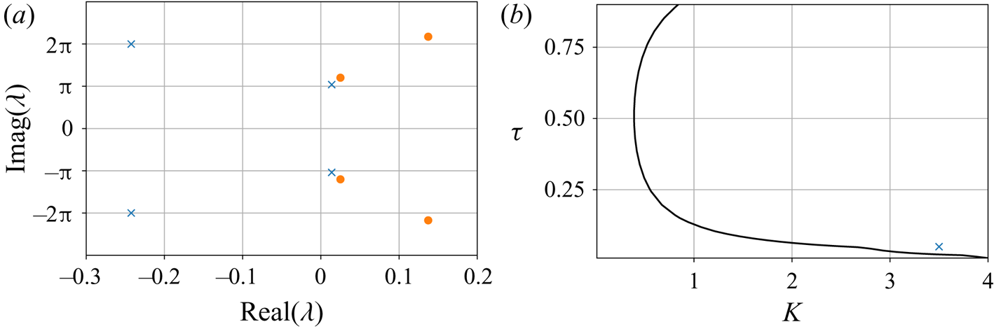
Now that many aspects of the phase-sensitivity analysis have been presented, we consider one more parameter regime. For the baseline case considered so far, the steady state  $(u,p)=(0,0)$ has one pair of unstable eigenvalues around the primary pure-acoustic angular frequency of
 $\omega ={\rm \pi}$, as shown in figure 6(a). This figure also shows stable eigenvalues at the first harmonic of this mode with an angular frequency of approximately
 $\omega =2{\rm \pi}$. The result is a limit cycle that is primarily dominated by one frequency. To consider a limit cycle with two dominant frequencies, we can consider the neutral curve presented by Sayadi et al. (Reference Sayadi, Le Chenadec, Schmid, Richecoeur and Massot2014). For the flame location
 $x_f=0.2$, the neutral curve shown in figure 6(b) is obtained. We can see that around a flame strength of
 $K\approx 3$, a ‘kink’ develops in the neutral curve. As discussed by Sayadi et al. (Reference Sayadi, Le Chenadec, Schmid, Richecoeur and Massot2014), this ‘kink’ occurs because the secondary eigenvalue with
 $\omega \approx 2{\rm \pi}$ becomes more unstable than the fundamental mode. Therefore, to consider the effect of two frequencies, we now consider the case of
 $x_f=0.2$,
 $K=3.5$ and
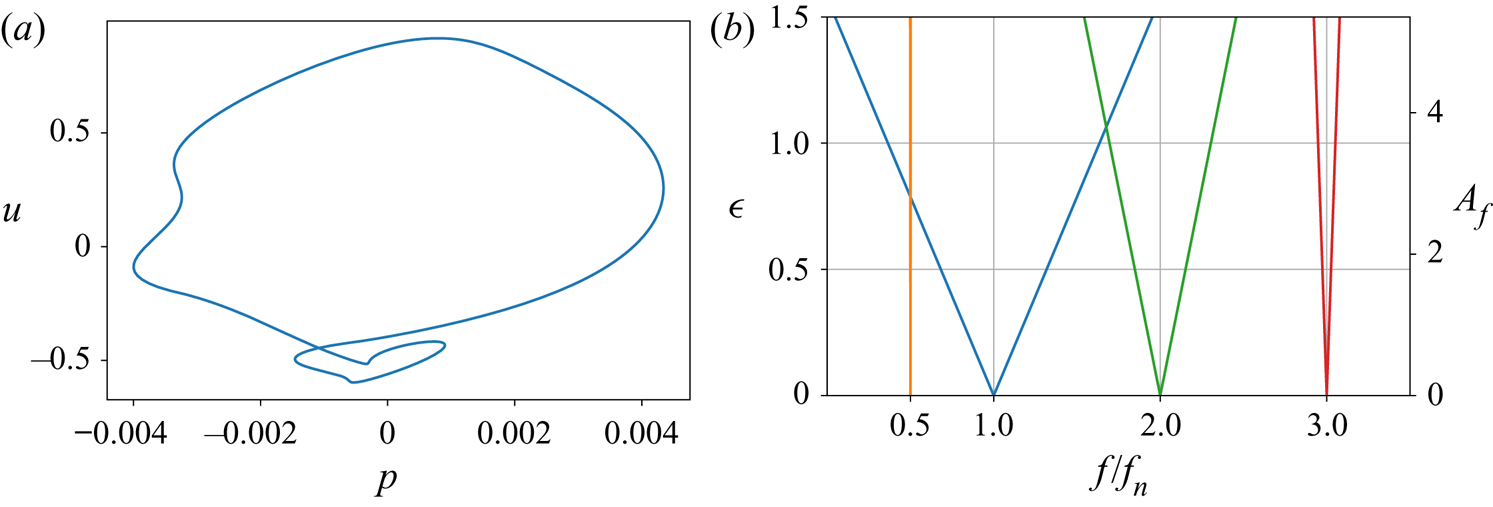
 $\tau =0.05$, which is shown in figure 6(b) to be located near the ‘kink.’ We note that for the parameter regime of this two frequency case, Sayadi et al. (Reference Sayadi, Le Chenadec, Schmid, Richecoeur and Massot2014) show that the mode shapes from a Galerkin approach show less agreement with a high fidelity approach that properly discretises the discontinuity at the flame. Therefore, as in our parametric study showcased in figure 5, we proceed with caution when interpreting the results. For these parameters, figure 6(a) shows that now both the fundamental and first harmonic are unstable, with the first harmonic being more unstable than the fundamental mode. As in the baseline case, this instability saturates into a limit cycle (see figure 7a), where the presence of a second frequency is evident in its ‘loop.’
(a) Eigenvalues for the one frequency (blue crosses) and two frequency (orange circles) systems. (b) Neutral curve for  $x_f=0.2$.

(a) Limit cycle for the multiple frequency system. (b) Arnold tongues for  $1:2$ (orange),
 $1:1$ (blue),
 $2:1$ (green) and
 $3:1$ (red) synchronisation for our multiple frequency system.

Figure 7(b) shows the Arnold tongues for  $1:2$,
 $1:1$,
 $2:1$ and
 $3:1$ synchronisation for the same forcing used to produce figure 4(b). We see that
 $1:1$ phase locking is easier in this system than the baseline. The reason for this could be attributed to the fact that figure 5(b) suggests that synchronisation becomes easier as the flame time delay is decreased. However, it is also evident that
 $2:1$ phase locking is now more easily achievable than
 $3:1$ phase locking which cannot arise from the smaller flame time delay alone. The reason for the increased
 $2:1$ synchronisability for this double frequency case can be viewed as a direct consequence of having a more dominant first harmonic in the nonlinear solution. This translates into an adjoint solution that contains more content at this frequency, which in turn leads to higher synchronisability via the phase-coupling function.
We conclude our study by considering the potential speedups available over using fully non-simulations to find the Arnold tongues. For both methods, a limit-cycle solution must first be found. Once this is found, we can estimate the subsequent cost of each analysis as follows. For both the phase sensitivity and fully nonlinear methods, the main cost involved is from solving either the nonlinear or adjoint equations, with any post processing, such as obtaining the phase coupling function, being negligible. If we assume that the nonlinear and adjoint equations take the same amount of time  $t_{solve}$ to be solved, then the total time of the phase-sensitivity method is
 $C_{p.s.}=2t_{solve}$. For the nonlinear approach, if
 $n_{f}$ frequencies and
 $n_{A}$ amplitudes are used, then the total time will be
 $C_{n.l.}=n_{f}n_{A} t_{solve}$. Therefore, the speedup using the phase-sensitivity approach is
 $Sp=C_{n.l.}/C_{p.s.}=n_{f}n_{A}/2$. For example, if
 $n_{f}=n_{A}=10$, then the phase-sensitivity function approach will be approximately 50 times faster; a substantial speedup.
It is worth mentioning that the argument above does not take into account the fact that the nonlinear approach will have only yielded the Arnold tongue for one particular forcing function and one choice of  $n:m$ phase locking. If additional forcing functions or
 $n:m$ phase lockings are to be examined, then each case will call for another
 $C_{n.l.}$ time-units. However, the phase-sensitivity function does not depend on the exact form of the forcing function or phase-locking type considered, and therefore all subsequent analysis will be essentially free compared with the initial cost. These considerations further make the phase-sensitivity function an efficient choice for determining the phase properties of a Floquet-stable system close to its limit cycle. Whilst adjoint approaches can be expensive in terms of memory, the fact that the phase-sensitivity function is the adjoint neutral-Floquet mode means that it can be obtained using simulations over just one period of the limit cycle using an algorithm such as that presented by Barkley & Henderson (Reference Barkley and Henderson1996). Even though we do not take this approach here, using such a method could be critically important in rendering this analysis feasible for larger, memory-intensive systems.
6. Conclusion
We have performed phase-reduction analysis to study the phase-synchronisation properties of the thermoacoustic system in a Rijke tube with respect to the limit cycle produced by its instability. By reducing the phase dynamics to a scalar equation for the phase, we are able to reveal the effects of weak external forcing on the phase through the phase-sensitivity function. The fact that this phase-sensitivity function can be found through integration of the adjoint equation, and does not depend on the exact form of the external forcing, makes this analysis particularly efficient and generalisable. We used the phase description to map out the regions where  $m:n$ phase locking can occur and identify the optimal positions along the Rijke tube where pressure actuation can result in synchronisation. The current study highlights the usefulness of phase-sensitivity analysis for thermoacoustic problems, especially as an additional tool for designing open-loop control strategies via harmonic forcing.
Whilst keeping in mind that this method is not directly applicable to turbulent systems, unstable limit cycles or for determining synchronisation behaviour far from a limit cycle, the present phase-reduction analysis for a Rijke tube can be extended to suitable, more complex thermoacoustic simulations without major change. For future work, it would be interesting to first extend the analysis to a higher fidelity model of a Rijke tube (Sayadi et al. Reference Sayadi, Le Chenadec, Schmid, Richecoeur and Massot2014) that explicitly treats the jump conditions at the flame, allowing for the phase dynamics near the flame, and for higher flame strengths, to be accurately quantified. Further to this, including the effects of a mean-flow in the Rijke tube model, and introducing velocity-based forcing, would also be beneficial in matching the synchronisation characteristics of some experimental set-ups. Applying phase techniques to more complex models including flame chemistry and more complex geometries would allow phase-sensitivity analysis to play a role in the control of instabilities arising from more realistic combustion systems.
Acknowledgements
We would like to thank the referees, whose helpful comments in the peer-review process improved this paper.
Funding
This work was supported by the US Air Force Office of Scientific Research (FA9550-16-1-0650, FA9550-21-1-0178; Program Managers: Douglas Smith and Gregg Abate).
Data availability statement
The numerical code that supports the findings of this study is openly available at http://doi.org/10.5281/zenodo.4981470 (Skene & Taira Reference Skene and Taira2021).
Declaration of interests
The authors report no conflict of interest.
Appendix A. Mathematical details
For a DDE in the form (2.4), we see that the initial condition (initial history) must be specified over  $-\tau \leq t\leq 0$ for the subsequent solution to be uniquely defined. In general, to propagate a state at time
 $t_0$ forward, we need the solution to the DDE over
 $-\tau \leq t-t_0\leq 0$. Therefore, it is helpful to think of the state as a function of the time-delay
 $\phi \in [-\tau,0]$, i.e. for each time
 $t$, we write a solution to the equation as
 $\boldsymbol {y}_t(\phi )=\boldsymbol {y}(t+\phi )$ (Hale Reference Hale1977). In this manner, the solution to the DDE is a function and we can formally write
 $\boldsymbol {y}_t\in \mathcal {C}([-\tau,0])$. An evolution equation can be found directly for the function
 $\boldsymbol {y}_t(\phi )$ and is defined piecewise as
 \begin{equation} \frac{\textrm{d} \boldsymbol{y}_t(\phi)}{\textrm{d}t}=\begin{cases} \dfrac{\textrm{d} \boldsymbol{y}_t(\phi)}{\textrm{d}\phi} & \textrm{if} \ \phi \in[-\tau,0),\\ \boldsymbol{f}(t,\boldsymbol{y}_t(0))+\boldsymbol{g}(t-\tau,\boldsymbol{y}_t(-\tau))+\epsilon \boldsymbol{h}(t) & \textrm{if} \ \phi=0. \end{cases} \end{equation}
Similarly, the linearised equations (with  $\epsilon =0$) can be written as
 ${\textrm {d} \boldsymbol {y}_t(\phi )}/{\textrm {d}t}=\mathcal {A}\boldsymbol {y}_t(\phi )$ where the linear operator
 \begin{equation} \mathcal{A}\boldsymbol{y}_t(\phi)=\begin{cases} \dfrac{\textrm{d} \boldsymbol{y}_t(\phi)}{\textrm{d}\phi} & \textrm{if} \ \phi \in[-\tau,0),\\ \boldsymbol{A}_1(t)\boldsymbol{y}_t(0)+\boldsymbol{A}_2(t)\boldsymbol{y}_t(-\tau) & \textrm{if} \ \phi=0. \end{cases} \end{equation}
As we are using an infinite-dimensional description for solutions to our DDE, care is needed when defining the adjoint. For finite-dimensional systems the adjoint is defined via an inner product because the direct and adjoint variables are defined in the same space, e.g.  $\mathbb {R}^N$. However, for a DDE, the direct variable
 $\boldsymbol {y}_t(\phi )\in \mathcal {C}([-\tau,0])$, whereas the adjoint
 $\boldsymbol {y}^{\dagger} _t(\phi )\in \mathcal {C}([0,\tau ])$. Hence, to define the adjoint, a bilinear form
 $V(\mathcal {C}([0,\tau ]),\mathcal {C}([-\tau,0]))\rightarrow \mathbb {R}$ is needed (see Wischert et al. Reference Wischert, Wunderlin, Pelster, Olivier and Groslambert1994; Simmendinger et al. Reference Simmendinger, Wunderlin and Pelster1999; Kotani et al. Reference Kotani, Yamaguchi, Ogawa, Jimbo, Nakao and Ermentrout2012; Novičenko & Pyragas Reference Novičenko and Pyragas2012). In terms of our functional notation, the bilinear form (3.3) can be written as
 \begin{equation} \langle\boldsymbol{a}_t(\phi),\boldsymbol{b}_t(\phi)\rangle=\boldsymbol{a}_t(0)^\textrm{T}\boldsymbol{b}_t(0)+\int_{-\tau}^0\boldsymbol{a}_t(\xi+\tau)^\textrm{T}\boldsymbol{A}_2(t+\tau+\xi)\boldsymbol{b}_t(\xi)\,\textrm{d}\xi. \end{equation}
The main steps of how to find the adjoint operator are now given and mainly follows the derivation available in Rand (Reference Rand2012).
To define the adjoint, we require that the bilinear form between a direct state and its adjoint (dual) state is constant in time (Simmendinger et al. Reference Simmendinger, Wunderlin and Pelster1999). Formally, this means that
 \begin{equation} \frac{\textrm{d}}{\textrm{d}t}\langle\boldsymbol{a}_t(\phi),\boldsymbol{b}_t(\phi)\rangle=0. \end{equation}
Using definition (A3), along with the fact that  ${\textrm {d} \boldsymbol {y}_t(\phi )}/{\textrm {d}t}=\mathcal {A}\boldsymbol {y}_t(\phi )$ and the definition
 $-{\textrm {d} \boldsymbol {y}^{\dagger} _t(\phi )}/{\textrm {d}t}=\mathcal {A}^{\dagger} \boldsymbol {y}^{\dagger} _t(\phi )$, where
 $\mathcal {A}^{\dagger}$ is the yet to be found adjoint operator, we have
 \begin{align} \frac{\textrm{d}}{\textrm{d}t}\langle\boldsymbol{a}_t(\phi),\boldsymbol{b}_t(\phi)\rangle &= \langle\boldsymbol{a}_t(\phi),\mathcal{A}\boldsymbol{b}_t(\phi)\rangle -\langle\mathcal{A}^{\dagger}\boldsymbol{a}_t(\phi),\boldsymbol{b}_t(\phi)\rangle\nonumber\\ &\quad + \int_{-\tau}^0\boldsymbol{a}_t(\xi+\tau)^\textrm{T}\frac{\textrm{d}\boldsymbol{A}_2(t+\tau+\xi)}{\textrm{d}\xi}\boldsymbol{b}_t(\xi)\,\textrm{d}\xi. \end{align}
We see that for no-time delay, setting this expression to zero gives the classic adjoint condition that  $\langle \boldsymbol {a}_t(\phi ),\mathcal {A}\boldsymbol {b}_t(\phi )\rangle = \langle \mathcal {A}^{\dagger} \boldsymbol {a}_t(\phi ),\boldsymbol {b}_t(\phi )\rangle$. However, for a time-delayed system, the infinite-dimensional nature gives an extra term owing to the memory of the system. Again using the inner product (A3), we have that
 \begin{align} \langle\boldsymbol{a}_t(\phi),\mathcal{A}\boldsymbol{b}_t(\phi)\rangle &=\boldsymbol{a}_t(0)^\textrm{T}\mathcal{A}\boldsymbol{b}_t(0)\nonumber\\ &\quad +\int_{-\tau}^0\boldsymbol{a}_t(\xi+\tau)^\textrm{T}\boldsymbol{A}_2(t+\tau+\xi)\mathcal{A}\boldsymbol{b}_t(\xi)\,\textrm{d}\xi, \end{align}
which upon using the definition of  $\mathcal {A}$ (A2) becomes
 \begin{align} \langle\boldsymbol{a}_t(\phi),\mathcal{A}\boldsymbol{b}_t(\phi)\rangle &=\boldsymbol{a}_t(0)^\textrm{T}(\boldsymbol{A}_1(t)\boldsymbol{b}_t(0)+\boldsymbol{A}_2(t)\boldsymbol{b}_t(-\tau))\nonumber\\ &\quad +\underbrace{\int_{-\tau}^0\boldsymbol{a}_t(\xi+\tau)^\textrm{T}\boldsymbol{A}_2(t+\tau+\xi)\frac{\textrm{d}\boldsymbol{b}_t(\xi)}{\textrm{d}\xi}\,\textrm{d}\xi}_{I}. \end{align}
The integral term  $I$ in (A7) can be rearranged using integration by parts to give
 \begin{align} I &=[\boldsymbol{a}_t(\xi+\tau)^\textrm{T}\boldsymbol{A}_2(t+\tau+\xi)\boldsymbol{b}_t(\xi)]_{-\tau}^0\nonumber\\ &\quad -\int_{-\tau}^0\left[\frac{\textrm{d}\boldsymbol{a}_t(\xi+\tau)}{\textrm{d}\xi}\right]^\textrm{T} \boldsymbol{A}_2(t+\tau+\xi)\boldsymbol{b}_t(\xi)\,\textrm{d}\xi\nonumber\\ &\quad -\int_{-\tau}^0\boldsymbol{a}_t(\xi+\tau)^\textrm{T}\frac{\textrm{d}\boldsymbol{A}_2(t+\tau+\xi)}{\textrm{d}\xi}\boldsymbol{b}_t(\xi)\,\textrm{d}\xi. \end{align}
Combining all the terms in (A7), using the integral term in this form gives
 \begin{align} \langle\boldsymbol{a}_t(\phi),\mathcal{A}\boldsymbol{b}_t(\phi)\rangle &=[\boldsymbol{A}_1(t)^\textrm{T}\boldsymbol{a}_t(0)+\boldsymbol{A}_2(t+\tau)\boldsymbol{a}_t(\tau)]^\textrm{T}\boldsymbol{b}_t(0)\nonumber\\ &\quad +\int_{-\tau}^0\left[-\frac{\textrm{d}\boldsymbol{a}_t(\xi+\tau)}{\textrm{d}\xi}\right]^\textrm{T} \boldsymbol{A}_2(t+\tau+\xi)\boldsymbol{b}_t(\xi)\,\textrm{d}\xi\nonumber\\ &\quad -\int_{-\tau}^0\boldsymbol{a}_t(\xi+\tau)^\textrm{T}\frac{\textrm{d}\boldsymbol{A}_2(t+\tau+\xi)}{\textrm{d}\xi}\boldsymbol{b}_t(\xi)\,\textrm{d}\xi, \end{align}
which we recognise as
 \begin{align} \langle\boldsymbol{a}_t(\phi),\mathcal{A}\boldsymbol{b}_t(\phi)\rangle &=\langle\mathcal{A}^{\dagger}\boldsymbol{a}_t(\phi),\boldsymbol{b}_t(\phi)\rangle\nonumber\\ &\quad -\int_{-\tau}^0\boldsymbol{a}_t^\textrm{T}(\xi+\tau) \frac{\textrm{d}\boldsymbol{A}_2(t+\tau+\xi)}{\textrm{d}\xi}\boldsymbol{b}_t(\xi)\,\textrm{d}\xi, \end{align}
where the adjoint operator  $\mathcal {A}^{\dagger}$ is now defined as
 \begin{equation} \mathcal{A}^{\dagger}\boldsymbol{y}_t^{\dagger}(\phi)=\begin{cases} -\dfrac{\textrm{d} \boldsymbol{y}_t^{\dagger}(\phi)}{\textrm{d}\phi} & \textrm{if} \ \phi \in(0,\tau],\\ \boldsymbol{A}_1^\textrm{T}(t)\boldsymbol{y}_t^{\dagger}(0)+\boldsymbol{A}_2^\textrm{T}(t+\tau)\boldsymbol{y}_t^{\dagger}(\tau) & \textrm{if} \ \phi=0. \end{cases} \end{equation}
Substituting (A10) into (A5) then shows that the bilinear form between a direct state and its dual remains constant in time.
For a  $T$-periodic system close to the limit cycle
 $\boldsymbol {y}^{LC}_t(\phi )$, a state can be written as
 $\boldsymbol {y}_t(\phi )=\boldsymbol {y}^{LC}_t(\phi )+\epsilon \boldsymbol {y}'_t(\phi )$. By the Floquet theorem (Floquet Reference Floquet1883), which carries over to delay differential equations (Simmendinger et al. Reference Simmendinger, Wunderlin and Pelster1999), the perturbation
 $\boldsymbol {y}'_t(\phi )$ can be written as
 \begin{equation} \boldsymbol{y}'_t(\phi) = \sum_i c_i\exp(\lambda_i t)\boldsymbol{y}^i_t(\phi), \end{equation}
where the Floquet modes  $\boldsymbol {y}^i_t(\phi )$ are
 $T$-periodic functions,
 $c_i$ are coefficients and
 $\lambda _i\in \mathbb {C}$ are the Floquet multipliers. This allows the idea of stability to be carried forward to periodic systems. If
 $\textrm {real}(\lambda _i)\leq 0$ for all
 $i$, then the limit cycle is stable and all perturbed states eventually return to the limit cycle (but generally with a phase shift), which is a necessary condition for our phase definition. For an autonomous system, there is always one neutral Floquet mode (
 $i=0$) with
 $\lambda _0=0$. Moreover, the neutral mode shape can be found directly from the limit cycle solution via
 $\boldsymbol {y}^0_t(\phi )=\dot {\boldsymbol {y}}^{LC}_t(\phi )$ (Simmendinger et al. Reference Simmendinger, Wunderlin and Pelster1999). It can be seen that this mode represents the phase shift because a Taylor expansion gives
 $\boldsymbol {y}^{LC}_{t+\alpha }(\phi )\approx \boldsymbol {y}^{LC}_{t}+\alpha \dot {\boldsymbol {y}}^{LC}_t(\phi )$. Therefore, it is natural to use Floquet theory to understand the phase-sensitivity function. We now demonstrate this using a similar approach to that of Novičenko & Pyragas (Reference Novičenko and Pyragas2012).
Consider the perturbed equation (2.4). Because the forcing term is small, we can seek the solution in the form  $\boldsymbol {y}_t(\phi )=\boldsymbol {y}^{LC}_t(\phi ) + \epsilon \boldsymbol {y}_t'(\phi )$. By linearising (2.4), we have that this perturbation is governed by the equation
 $\dot {\boldsymbol {y}}_t'(\phi )=\mathcal {A}\boldsymbol {y}_t'(\phi )+\mathcal {A}^h\boldsymbol {y}_t'(\phi )$, where
 \begin{equation} \mathcal{A}^h\boldsymbol{y}_t(\phi)=\begin{cases} 0 & \textrm{if} \ \phi \in[-\tau,0),\\ h(t) & \textrm{if} \ \phi=0, \end{cases} \end{equation}
and  $\mathcal {A}$ is defined as (A2) from before. Now, because the perturbation is small and remains close to the limit cycle, we can use the Floquet theorem to express the perturbation in the form
 \begin{equation} \boldsymbol{y}'_t(\phi)=\epsilon\sum_i c_i(t)\boldsymbol{y}^i_t(\phi). \end{equation}
From our previous discussion, we know that only the  $i=0$ Floquet mode has the ability to change the phase of the system. Therefore, using a similar argument as before for each time
 $t$, the phase for the perturbed system must be
 $\theta =\omega _nt+\epsilon \omega _n c_0(t)$, giving its evolution equation as
 $\dot {\theta } = \omega _n + \epsilon \omega _n\dot {c}_0(t)$.
Now that we have found the phase equation in terms of the time-dependent coefficients of the Floquet expansion, we can use the adjoint to relate  $\dot {c}_0(t)$ to the forcing term
 $h(t)$. To do this, we first recognise that even though the Floquet modes are not orthogonal, the direct and adjoint Floquet modes form a bi-orthogonal set under our bilinear form (Simmendinger et al. Reference Simmendinger, Wunderlin and Pelster1999). In other words, with an appropriate normalisation of the adjoint,
 $\langle \boldsymbol {y}^{i,{\dagger} }_t(\phi ),\boldsymbol {y}^j_t(\phi )\rangle =d_{i,j}\delta _{i,j}$, where
 $d_{i,j}$ are coefficients that depend on the normalisation and
 $\delta _{i,j}$ is the Kronecker delta. Note that for
 $i=j=0$, this implies that
 $\langle \boldsymbol {y}^{0,{\dagger} }_t(\phi ),\dot {\boldsymbol {y}}^{LC}_t(\phi )\rangle =\omega _n$, where we have chosen the normalisation
 $d_{0,0}=\omega _n$. Using this biorthogonality, we can take the bilinear form of (A14) with
 $\boldsymbol {y}^{0,{\dagger} }_t(\phi )$ to find
 $c_0(t)$ as
 $\langle \boldsymbol {y}^{0,{\dagger} }_t(\phi ),\boldsymbol {y}'_t(\phi )\rangle =\epsilon \omega _n c_0(t)$. To find
 $\dot {c}_0(t)$, we differentiate this expression with respect to time. Using the already shown result that the time derivative of the contribution to this bilinear form from the unperturbed dynamics is zero, we obtain
 \begin{equation} \epsilon\omega_n\dot{c}_0(t) = \langle \boldsymbol{y}^{0,{\dagger}}_t(\phi),\mathcal{A}^h\boldsymbol{y}'_t(\phi)\rangle, \end{equation}
which, from the definition (A13), becomes  $\omega _n\dot {c}_0(t)=\boldsymbol {y}^{0,{\dagger} }_t(0)^\textrm {T}h(t)$. Hence, dropping the
 $i=0$ superscript, the phase equation is (3.1) with
 $Z(\theta )=\boldsymbol {y}^{{\dagger} }_{t=\theta /\omega _n}(0)$.