




1. Introduction
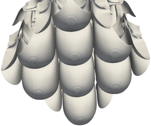
Mammatus clouds are a fascinating meteorological phenomenon. Deriving their name from mamma, the Latin for ‘breast’, mammatus clouds are pendulous blobs, typically found hanging underneath cumulonimbus anvils (a photograph is reproduced in figure 1 and a schematic shown in figure 2a). Their origin has been a mystery, and several explanations, in the form of plausible physical arguments, have been suggested (listed in the review by Schultz et al. (Reference Schultz, Kanak, Straka, Trapp, Gordon, Zrnić, Bryan, Durant, Garrett, Klein and Lilly2006)). A promising explanation is the fallout of ice particles or water droplets from the cumulus anvil into the subsaturated air below, suggested first almost a hundred years ago (Troeger Reference Troeger1921, cited by Schultz et al. Reference Schultz, Kanak, Straka, Trapp, Gordon, Zrnić, Bryan, Durant, Garrett, Klein and Lilly2006), followed by the sublimation/evaporation of these hydrometeors. This causes the layer of air just below the cloud (the ‘sub-cloud layer’) to become denser than the dry air below it. This density ‘overhang’ can then cause an instability, which can lead to the formation of mammatus clouds (Kanak & Straka Reference Kanak and Straka2006). This mechanism, however, does not always lead to mammatus clouds (Schultz et al. Reference Schultz, Kanak, Straka, Trapp, Gordon, Zrnić, Bryan, Durant, Garrett, Klein and Lilly2006). We analyse this proposed mechanism in detail via linear stability analysis and nonlinear simulations, in order to clarify the conditions under which mammatus-like lobes can form. We formulate a simplified description of the problem in terms of only the amount of liquid water in the anvil, and the size of the droplets making up the liquid water content, to provide an argument for why evaporative cooling by itself does not necessarily result in mammatus-like lobes. We also find that the size of the water droplets matters more than the total amount of liquid water.
A photograph of mammatus clouds seen on 26 June 2012 in Regina, Saskatchewan, Canada, following a severe storm warning and tornado watch. Taken by Craig Lindsay. Reproduced from Wikipedia (Creative Commons Licence).

(a) A schematic of a typical mammatus cloud forming under a cumulonimbus anvil. (b,c) The idealisation of the red box in (a) at  $t=0$ (b) and
 $t>0$ (c). The vertical direction is along
 $z$. The horizontal direction(s) (
 $x$ in two dimensions,
 $x,y$ in three dimensions) are assumed periodic. The upper half of the domain of depth
 $\delta z^{0}$ has saturated vapour and liquid droplets with an initial mixing ratio
 $r_l^{0}$. The lower half is initially dry (i.e. has no vapour). Both halves are at the same initial temperature
 $T_0$. Other thermodynamic constants are defined in the text. The liquid droplets that settle out of the anvil evaporate just under the anvil and cool the layer (in a lighter shade of grey). Schematic profiles of base density at the initial and a later time are also shown.

The instability of a layer of fluid rendered unstable because of settling has been studied by Yu, Hsu & Balachandar (Reference Yu, Hsu and Balachandar2013, Reference Yu, Hsu and Balachandar2014) and also by Burns & Meiburg (Reference Burns and Meiburg2012, Reference Burns and Meiburg2015). The latter studied the instability of a layer of silt-laden fresh water atop a layer of salty water. They characterised the instability that occurs in terms of the settling velocity and the stability ratio, and found that for large settling velocities, the instability is ‘leaky’, producing wisps of fluid that leak from the upper half. For small settling velocities, the two halves of the fluid form ‘finger-like’ protrusions into each other. The settling velocity thus decides whether the instability is of the Rayleigh–Taylor type (the leaky mode) or of the double-diffusive type (the fingering mode).
We apply the idea of settling-driven instabilities to mammatus cloud formation, where the settling component is the liquid/ice in the cumulonimbus anvil. The settling velocity is the terminal velocity of the ice/water hydrometeors. The major difference between this study and that of Burns & Meiburg (Reference Burns and Meiburg2012) is in the mechanism that causes the instability. In Burns & Meiburg (Reference Burns and Meiburg2012) the mass of the settling sediment is sufficient to cause a density overhang, whereas the total mass of the settling particles or droplets in terrestrial atmospheric conditions is too low to cause a significant density overhang by itself. The instability here is caused by the thermodynamics of evaporation/sublimation, which cools the ambient temperature below the cumulus anvil, and increases air density in that region. The necessary condition we find for our instability-driven mechanism is in broad agreement with Kanak, Straka & Schultz (Reference Kanak, Straka and Schultz2008), who find from numerical simulations that the evaporation/sublimation of water droplets is crucial to the formation of mammatus clouds. Their study attempts to reproduce observations of mammatus clouds from specific atmospheric observations, and their simulations are performed with different scalars for liquid water and ice. We neglect the complexities of the different possible condensed states of water, and focus instead on the fluid mechanics of settling-driven instabilities.
The aim of our work is thus to study the interactions between the settling of the liquid field, the thermodynamics of phase change and the resulting buoyancy-driven flow. Since our objective is to clarify the fluid mechanics of the problem, rather than to reproduce specific observations, we ignore the complexities of the microphysics of freezing and work instead with only one condensed phase (which we will henceforth call ‘liquid’). We use linear stability analysis and simulations of the Boussinesq Navier–Stokes equations with vapour/liquid phase change. Our aim and approach are thus different from the numerical studies cited above. In § 2, we set up the problem and derive the non-dimensional equations we solve. In § 3, we report results from linear stability analysis of density profiles obtained by one-dimensional nonlinear evolution of the governing equations. In § 4, we describe the numerical method for solving the full equations, and the results of the simulations. In § 5, we discuss the results of §§ 3 and 4; compare the instability studied here with known fluid dynamical instabilities without and with a settling component; and discuss the limitations of the present approach to the study of mammatus clouds. We then conclude with some thoughts about future work.
2. Problem set-up
We take the cumulonimbus ‘anvil’ as our starting point (see figure 2b). Away from the updraught of cloudy fluid in the centre, there is a layer of cloud fluid, consisting of air saturated with water vapour and containing water droplets/ice particles forming a given liquid/ice density. The mammatus clouds of interest to us are ‘suspended’ under these anvils.
Our idealisation of the cumulonimbus anvil before the formation of the mammatus lobes is also shown (figure 2c). Our system consists of a layer of warm air that is saturated with water vapour and contains liquid water, below which lies a layer of dry air of the same temperature. For simplicity, we assume that the condensed phase in the cloud consists of only liquid droplets (i.e. no ice particles). We do this with the knowledge that the latent heat of vaporisation of water is about five times greater than the latent heat of fusion of ice, and is therefore the more significant reason for the density overhang.
Humid air is lighter than dry air. On the other hand, liquid water ‘settles’ in air. The amounts of liquid and vapour in air are given in terms of their mixing ratios  $\tilde {r}_{l}$ and
 $\tilde {r}_{v}$, respectively. The tilde indicates that these quantities are unnormalised (see (2.9) below). These are defined as
 \begin{equation} \tilde{r}_{i}=\rho_{i}/\rho_{d}, \end{equation}
where  $\rho _{d}$ is the density of the dry air component of the mixture and ‘
 $i$’ can be
 $l$ or
 $v$ for liquid or vapour, respectively. In other words,
 $\rho _{d,v,l}$ are the ‘partial densities’ of the three components of the mixture. The net density of the fluid is the sum of these partial densities:
 \begin{align} \rho & = {\rho_d + \rho_v + \rho_l} \nonumber\\ & =\rho_{d}\left(1+\tilde{r}_{v}+\tilde{r}_{l}\right). \end{align}
The above expression is exact. Further simplification is possible (see (2.6) below) if  $\tilde r_{v,l}\ll 1$, which is true of atmospheric conditions.
We employ the Boussinesq Navier–Stokes equations with a constant ambient temperature  $T_{0}$. The velocity field
 $\boldsymbol {u}$ is incompressible (
 $\boldsymbol{\nabla} \boldsymbol{\cdot} \boldsymbol {u}=0$). The liquid and vapour mixing ratios,
 $\tilde {r}_{v}$ and
 $\tilde {r}_{l}$, are advected with the fluid velocity, except that the liquid also settles with a velocity
 $\tilde {v}_{p}$. Temperature differences and vapour and liquid concentrations all contribute to the buoyancy, and thus to the flow driven by these buoyancy differences. Under the conditions we have chosen, the contribution from temperature differences has the greatest effect of these three. Note also that the background state, denoted by subscript 0, is assumed to be unchanging; in the atmosphere, this will not be the case, since, even in the absence of wind, the instability discussed below will develop simultaneously with the base density overhang shown in figure 2.
The buoyancy may be expressed in terms of the temperature and liquid and vapour mixing ratios as follows. We write the density of dry air in terms of the density  $\rho _{0}$ of the air outside the flow (assumed to contain no vapour). In the following, quantities
 $()_{d}$ pertain to dry air and
 $()_{v}$ to water vapour. Thus,
 $R_{d}$ is the gas constant for dry air and
 $R_{v}$ the gas constant for water vapour;
 $M_{d}$ is the molecular mass of dry air and
 $M_{w}$ is the molecular mass of water. We then have
 \begin{gather} p_{d}+p_{v} = p_{0}, \end{gather}
 \begin{gather}\rho_{d}R_{d}T+\rho_{d}\tilde{r}_{v}R_{v}T = \rho_{0}R_{d}T_{0}, \end{gather}
 \begin{gather}\rho_{d}R_{d}\left(1+\tilde{r}_{v}\left(1+\chi\right)\right)T = \rho_{0}R_{d}T_{0}, \end{gather}
where  $R_v=(1+\chi )R_d$ and
 $\chi +1=M_{d}/M_{w}$. We then have, assuming
 $\tilde {r}_{v},\tilde {r}_{l}\ll 1$,
 \begin{equation} \rho_{d} =\frac{T_{0}}{T}\rho_{0}\left(1-\tilde{r}_{v}\left(1+\chi\right)\right) \end{equation}
and
 \begin{equation} \frac{\rho}{\rho_{0}}=\frac{\rho_{d}}{\rho_{0}}\left(1+\tilde{r}_{v}+\tilde{r}_{l}\right)= \frac{T_{0}}{T}\left(1+\tilde{r}_{v}+\tilde{r}_{l}\right)\left(1-\tilde{r}_{v}\left(1+\chi\right)\right)= \frac{T_{0}}{T}\left(1-\chi\tilde{r}_{v}+\tilde{r}_{l}\right). \end{equation}
The buoyancy is proportional to the differences between the ambient density  $\rho _{0}$ and the local density, and is given by
 \begin{equation} B=g\left(1-\frac{\rho}{\rho_0}\right)=g\left(1-\frac{T_{0}}{T}\left(1-\chi\tilde{r}_{v}+\tilde{r}_{l}\right)\right) \approx g\left(\frac{T-T_{0}}{T_{0}}+\chi\tilde{r}_{v}-\tilde{r}_{l}\right),\end{equation}
where we have used the fact that  $T/T_0\approx 1$ when this term multiplies
 $\tilde {r}_v$ or
 $\tilde {r}_l$.
With this, the equations governing the motion, the temperature  $T$ and vapour and liquid mixing ratios
 $\tilde {r}_{v}$ and
 $\tilde {r}_{l}$ are
 \begin{gather} \left.\begin{aligned} \boldsymbol{\nabla}\boldsymbol{\cdot}\boldsymbol{u} = 0, \nonumber\\ \frac{\textrm{D}\boldsymbol{u}}{ \textrm{D} t} = -\frac{\boldsymbol{\nabla} p}{\rho_{0}}+g\boldsymbol{e}_z \left(\frac{T-T_{0}}{T_{0}}+\chi \tilde r_{v}- \tilde r_{l}\right)+\nu\nabla^{2}\boldsymbol{u}, \nonumber\\ \frac{ \textrm{D} T}{ \textrm{D} t} = \kappa\nabla^{2}T-\frac{L_{v}}{C_{p}}E, \nonumber\\ \frac{ \textrm{D}\tilde{r}_{v}}{ \textrm{D} t} = \kappa_{v}\nabla^{2}\tilde{r}_{v}+E, \nonumber\\ \frac{\textrm{D}\tilde{r}_{l}}{ \textrm{D} t} = \tilde{v}_{p}\frac{\partial\tilde{r}_{l}}{\partial z}+\kappa_{l}\nabla^{2}\tilde{r}_{l}-E, \end{aligned}\right\}\end{gather}
where  $\textrm {D}/ \textrm {D} t$ is the material derivative,
 $\kappa _{v}, \kappa _{l}$ and
 $\kappa$ are the diffusivities associated with vapour, liquid and temperature, respectively,
 $E$ is the rate of evaporation,
 $L_{v}$ is the enthalpy of vaporisation and
 $C_{p}$ is the specific heat at constant pressure. For the present work, we take
 \begin{equation} \nu =\kappa=\kappa_{v} \quad \textrm{and} \quad \kappa_{l} =0. \end{equation}
For air, the Prandtl number  $Pr=\nu /\kappa \approx 0.7$ and the Schmidt number for water vapour
 $Sc_{v}=\nu /\kappa _{v}\approx 0.66$. We use
 $Pr=Sc_{v}=1$ for simplicity. The diffusivity of the liquid water component is zero (see § 4 for the numerical method used), since the droplets that make up the liquid water content, being tens of micrometres in size, are too large for Brownian diffusion. We also find, from simulations that are not reported here, that similar results are obtained if the Schmidt number for the liquid
 $Sc_{l}=\nu /\kappa _{l}$ is set equal to one. It is important to note that a Schmidt number of one for the liquid component rules out ‘double’-diffusive instabilities, which are usually important in mixing-driven evaporatively cooled instabilities (and were also identified as the cause of the fingering instability in Burns & Meiburg (Reference Burns and Meiburg2012, Reference Burns and Meiburg2015)), as the cause of mammatus lobe formation.
2.1. Non-dimensionalised equations and initial conditions
Since the flow is buoyancy-driven, the buoyancy velocity  $\mathcal {U} = (g\mathcal {L} {\rm \Delta} T/T_0)^{1/2}$ is the appropriate velocity scale, where
 $\mathcal {L}$ is a length scale given by the size of the mammatus lobes. Together, these define the time scale
 $\mathcal {T}$. Other relevant scales are the scale of temperature variations
 ${\rm \Delta} T$ (which gives
 $\theta =(T-T_{0})/ {\rm \Delta} T$) and the saturation mixing ratio
 $r_{s}^{0}=r_{s}^{0}(T_{0})$ at a base temperature
 $T_{0}$. We write the non-dimensional equations as follows:
 \begin{gather} \frac{ \textrm{D}\boldsymbol{u}}{ \textrm{D} t} = -\boldsymbol{\nabla} p + \boldsymbol{e}_z \left(\theta+r^{0}\left(\chi r_{v}-r_{l}\right)\right)+\frac{1}{Re}\nabla^{2}\boldsymbol{u}, \end{gather}
 \begin{gather}\frac{ \textrm{D}\theta}{ \textrm{D} t} =\frac{1}{Re\,Pr}\nabla^{2}\theta-L_{1}E, \end{gather}
 \begin{gather}\frac{ \textrm{D} r_{v}}{ \textrm{D} t} =\frac{1}{Re\,Sc_{v}}\nabla^{2}r_{v}+E, \end{gather}
 \begin{gather}\frac{ \textrm{D} r_{l}}{ \textrm{D} t} =v_{p}\frac{\partial r_{l}}{\partial z}+\frac{1}{Re\,Sc_{l}}\nabla^{2}r_{l}-E. \end{gather}
In the above,  $Re=\mathcal {UL}/\nu$ is the Reynolds number. The number
 $r^{0}=r_{s}^{0}T_{0}/ {\rm \Delta} T$ is a stability ratio and governs the relative contributions of the water components and the temperature difference to the buoyancy, and
 $v_p=\tilde {v}_p/\mathcal {U}$ is the non-dimensional settling velocity. The evaporation rate
 $E$ has also been non-dimensionalised with the inverse of the time scale
 $\mathcal {T}$. We choose a base temperature
 $T_{0}=273$ K, which is a representative temperature at which mammatus clouds are seen (see table 1 in Schultz et al. (Reference Schultz, Kanak, Straka, Trapp, Gordon, Zrnić, Bryan, Durant, Garrett, Klein and Lilly2006)). For this base temperature,
 $r^{0}=1.2285$. The parameter
 $L_{1}=(L_{v}r_{s}^{0})/(C_{p} {\rm \Delta} T)$ is the non-dimensional latent heat of vaporisation. We point out again that we consider only liquid water droplets and not ice particles. A condensed phase made entirely of ice would increase the latent heating by about
 $15\,\%$ because of the additional enthalpy of fusion. We use the value for the enthalpy of vaporisation of water of
 $L_v=2.5\times 10^{6}$. The dimensional length scale and time scale are chosen so as to make the non-dimensional
 $v_p = 1.0$ for
 $a_0=50~\mathrm {\mu }$m. This fixes the length scale at
 $\mathcal {L}\approx 8$ m. The time scale is then
 $\mathcal {T}=L/ \tilde {v}_{p} \approx 14$ s. For
 $r_l^{0} = 0.3$, this makes the non-dimensional
 $\tau _s \approx 2.86$ (see (2.22)).
For these values, along with the kinematic viscosity  $\nu =10^{-5}~\textrm {m}^{2}~\textrm {s}^{-1}$, the Reynolds number
 $Re={O}(10^{7})$. Since numerical simulations at such high Reynolds numbers are not feasible, we use an artificially low value of
 $Re$. The linear stability results (§ 3.2) across varying Reynolds numbers suggest that this is reasonable. Note also that since we do all our calculations in non-dimensional units, the only difference in simulations at a different length scale will be the magnitude of the Reynolds number.
The expressions for the phase change rate  $E$ are model-dependent. We choose the simplest non-equilibrium model (Shaw et al. Reference Shaw, Reade, Collins and Verlinde1998; Kumar, Schumacher & Shaw Reference Kumar, Schumacher and Shaw2013) given, in non-dimensional units, as
 \begin{equation} E=-\mathcal{H}\frac{1}{\tau_{s}}\left(\frac{r_{v}}{r_{s}}-1\right), \end{equation}
where  $\tau _{s}$ is the time scale for phase relaxation (in units of
 $\mathcal {T}$) and the function
 $\mathcal {H}$ is
 \[ \mathcal{H}=\begin{cases} 1 & \mbox{if the parcel is saturated, or if liquid is evaporating},\\ 0 & \mbox{if the parcel is unsaturated}. \end{cases} \]
The saturation vapour density  $r_{s}$ is a strong function of temperature (see e.g. Bohren & Albrecht Reference Bohren and Albrecht1998, chap. 5.3):
 \begin{equation} \frac{r_{s}\left(T\right)}{r_{s}^{0}}=\text{exp}\left[\frac{L_{v}}{R_{v}} \left(\frac{1}{T_{0}}-\frac{1}{T}\right)\right].\end{equation}
The equation can be simplified if we assume that deviations from the base temperature are small. We then get  $r_{s}/r_{s}^{0}\approx \text {exp}(L_{2}\theta )$, where
 \begin{equation} L_{2}=\frac{L_{v} {\rm \Delta} T}{R_{v}T_{0}^{2}}. \end{equation}
In two dimensions, simulations are done in a domain  $[-L_x/2,L_x/2]\times [0,L_z]$; in three dimensions, in a domain
 $[-L_x/2,L_x/2]\times [-L_y/2,L_y/2]\times [0,L_z]$. At
 $t=0$, the horizontal interface separating the cloudy anvil from the dry air is at
 $z=L_z/2$. The unperturbed system is given by
 \begin{gather}\left.\begin{aligned} \theta = 0, \nonumber\\ \boldsymbol{u} = 0, \nonumber\\ r_{v} =\begin{cases} 1, & z>L_z/2,\\ 0, & z<L_z/2, \end{cases} \nonumber\\ r_{l} = \begin{cases} r_{l}^{0}+\textrm{noise} , & L_z/2+\delta z^{0}>z>L_z/2,\\ 0 & \text{otherwise.} \end{cases} \end{aligned}\right\} \end{gather}
In the simulations in one dimension in § 3, we move to a coordinate frame  $z^{\prime } {=z-L_z/2} \subset [-L_z/2,L_z/2]$, with the interface at
 $t=0$ at
 $z^{\prime } = 0$.
We perturb the system in two ways, results from which are presented in § 4. In the first way, the interface remains horizontal, but we add noise externally to  $r_l^{0}$. Second, the interface itself is perturbed sinusoidally with a wavenumber in the horizontal direction in addition to the noise added to
 $r_l^{0}$. Our simulation box is of height
 $L_z$, and the initial anvil depth is
 $\delta z^{0}$. The interface is therefore perturbed about
 $z=L_z/2$ with an amplitude
 $\xi$:
 \begin{gather} \left.\begin{aligned}\theta = 0, \notag\\ \boldsymbol{u} = 0, \nonumber\\ r_{v} = \begin{cases} 1, & z>L_z/2+\xi\,\text{cos}\left(k_x x \right)\text{cos}\left(k_y y \right),\\ 0, & z<L_z/2+\xi\,\text{cos}\left(k_x x \right)\text{cos}\left(k_y y \right), \end{cases} \nonumber\\ r_{l} =\begin{cases} r_{l}^{0} + \textrm{noise}, & L_z/2+\delta z^{0}>z> L_z / 2 + \xi \cos(k_x x) \cos(k_y y),\\ 0 & \text{otherwise.} \end{cases} \end{aligned}\right\} \end{gather}
Therefore, the horizontal wavelengths at which the interface is perturbed are  $\lambda _x = 2{\rm \pi} /k_x$ and
 $\lambda _y=2{\rm \pi} /k_y$ and the number of wavelengths in the simulation box (along
 $x$, say) is
 $L_x/\lambda _x=L_x k_x/2{\rm \pi}$.
The quantities  $r_{l}$,
 $\tau _{s}$ and
 $v_{p}$ are functions of the number density
 $n$ and size
 $a_{0}$ of the droplets making up the condensed phase, as explained below. Therefore, only two of these three are independent parameters:
 \begin{gather} r_{l}^{0} \sim na_{0}^{3}, \end{gather}
 \begin{gather}\tilde{v}_p = (2{\rho_w a_0^{2} g})/({9 \rho_d \nu}), \end{gather}
 \begin{gather}\tilde{\tau}_s = \frac{C \rho_s^{0}}{4{\rm \pi} n a_0}, \end{gather}
where  $C$ is a dimensional constant with units of
 $\textrm {m}~\textrm {s}~\textrm {kg}^{-1}$ (see e.g. Kumar et al. Reference Kumar, Schumacher and Shaw2013). For
 $T_0=273~\textrm {K}$,
 $C=1.5\times 10^{7}~\textrm {m}~\textrm {s}~\textrm {kg}^{-1}$. As droplets settle out of the anvil and shrink, both the settling velocity and
 $\tau _s$ change as a result of the decreasing droplet radius. We assume that
 $n$ is constant in time. This variation is taken into account in the two-dimensional (2-D) and three-dimensional (3-D) simulations in § 4, but ignored in § 3 for simplicity. This does not affect results significantly.
We note also that, in what follows, we report results as being for a (dimensional) droplet size. What we mean is that  $v_{p}$ and
 $\tau _{s}$ were calculated using this droplet size, and then non-dimensionalised using the length and time scales of § 2.1.
3. Parameters, scaling arguments and linear stability analysis
As the droplets settle into the dry ambient in the lower half of our domain, they evaporate, cooling the sub-cloud layer and making it denser than the dry air below it. This causes an instability which we aim to characterise. The problem, even in our simplified description, has several governing parameters. We list them in table 1.
(Non-dimensional) parameters in the problem.

Of these, the parameters  $L_1$,
 $L_2$ and
 $r_s^{0}$ are functions of the absolute temperature
 $T_{0}$. Schultz et al. (Reference Schultz, Kanak, Straka, Trapp, Gordon, Zrnić, Bryan, Durant, Garrett, Klein and Lilly2006) report that mammatus clouds are observed at temperatures ranging from
 $T_0=273$ K to
 $T_0=235$ K, with a majority of observations around
 $273$ K. We fix
 $T_0=273$ K.
As the liquid droplets settle out of the cloud anvil and into the sub-cloud air, the quantities of interest in the dynamics are the depth  $h$ of the resulting evaporatively cooled layer and the maximum density difference
 $\rho _{max}$, or the amplitude of the density overhang in the layer:
 \begin{gather} h = h \left(a_{0},r_{l}^{0},\delta z^{0}\right), \end{gather}
 \begin{gather} \rho_{max} =\rho_{max}\left(a_{0},r_{l}^{0},\delta z^{0}\right). \end{gather}
In the above, the settling velocity of the liquid droplets is determined by their size  $a_0$. We recall that
 $v_p(a_0)$ and
 $\tau _s(a_0,r_l^{0})$ do not vary with time in this section. The total amount of liquid available to be evaporated, which will determine the total cooling, is given by the combination of
 $\delta z^{0}$ and
 $r_l^{0}$.
The functional relationships are obtained in this section using nonlinear simulations in one space dimension (the vertical) and time. The resulting density overhang then forms the base flow for our linear instability computations. For the discussion in this section we move to the coordinate system  $z^{\prime }=z-L_z/2$ with its origin at the lower interface between the anvil and the dry air. Representative density profiles that result from this process are shown in figure 3. It can be seen from these profiles that the depth of the density overhang increases steeply with increasing droplet radius
 $a_{0}$. On the other hand, the maximum density difference between the sub-cloud layer and the anvil (i.e. the horizontal extent of the spikes in the figure) increases only marginally with increasing liquid mixing ratio
 $r_{l}^{0}$. The variations are studied in § 3.1.
The evolution of the density profiles that result from different combinations of  $a_0$ and
 $r_l^{0}$. These profiles are obtained from nonlinear simulations in one space dimension (the vertical) and time. (a) The liquid mixing ratio
 $r_l$ and (b) the time variation of the density profiles, both for
 $a_0 = 60~\mathrm {\mu }$m,
 $r_l^{0}=0.5$. (c,d) Density profiles at
 $t=10$ for (c)
 $r_l^{0} = 0.1$ and (d)
 $r_l^{0} = 0.3$. Note that the liquid water has completely disappeared by
 $t=8$ for
 $a_0 = 60~\mathrm {\mu }$m, but the density overhang persists. For smaller
 $a_0$, the liquid takes longer to settle and evaporate; for larger
 $a_0$, the time required is shorter. In this figure and in figures 4 and 5, the values of
 $a_0$ correspond to the droplet size in micrometres that gives the corresponding values for
 $r_l^{0}$ and
 $\tau _s$ (see § 2.1 in the text).

3.1. Scaling arguments
We now study how the depth and amplitude of the density overhang vary with the droplet size and initial mixing ratio. We use the initial conditions of (2.19) with  $\xi =0$, and the anvil depth
 $\delta z^{0} = 1$. (This value of
 $\delta z^{0}$ is chosen so that all the liquid has evaporated in these simulations in a short time.) The liquid then settles and evaporates in the
 $z^{\prime }<0$ region. It is important to remember that this evaporation modifies the
 $z^{\prime }<0$ region and that this is a function of time.
3.1.1. Scaling of the depth of the density overhang
We first examine how the depth  $h$ of the density overhang (plotted by finding points at which the net density is greater by a threshold (
 $=0.001$) than the base state value of
 $1.0$ after all the liquid has evaporated) varies with the initial liquid mixing ratio in the anvil
 $r_{l}^{0}$ and the initial droplet radius
 $a_{0}$. The results are shown in figure 4. These plots suggest that for sufficiently large
 $a_0$ and
 $r_l^{0}$, the depth
 $h$ scales as
 $h \sim r_l^{0} (a_{0})^{3.6}$ over a small range of
 $a_0$. Thus, in this range, the depth of the density overhang grows faster than the settling velocity
 $v_p \sim a_0^{2}$ as
 $a_0$ increases. The time over which the droplets persist accounts for this. However, given that there is less than one decade along either axis, we do not use this power law to make any physical predictions (see e.g. Stumpf & Porter Reference Stumpf and Porter2012). For a given droplet size, the depth of the density overhang grows linearly with the initial liquid mixing ratio for
 $r_l > r_{l,cr}(a_0)$. For large
 $r_l^{0}$, the amount of liquid is sufficient to saturate the initial layers of fluid just below the anvil. This means that the remaining liquid water simply falls through the newly saturated layers. Thus, the larger the
 $r_l^{0}$, the further the liquid droplets can fall, explaining the linear behaviour. Between
 $a_0=20~\mathrm {\mu }$m and
 $a_0=40~\mathrm {\mu }$m, the density profiles have different time evolutions, but look similar when all the liquid has evaporated (i.e when figure 4 is plotted).
The depth of the cooled sub-cloud layer,  $h$, after all the liquid has settled and evaporated. (a) Depth
 $h$ increases linearly with the initial liquid mixing ratio,
 $r_l^{0}$, if the amount of liquid present is not very small. The sizes of the markers correspond to the droplet sizes. (b)Depth
 $h$ increases with droplet size,
 $a_0$, with a power-law dependence for large
 $r_l^{0}$ over a small range. The thicknesses of the dashed lines increase with increasing
 $r_l^{0}$. The thin solid line is
 $y\propto x^{3.6}$.

3.1.2. Scaling of the amplitude of the density overhang
Figure 5 shows the maximum density difference  $\rho _{max}-1$ between the density overhang and the base state. As with the depth of the density overhang, the maximum density difference varies linearly with
 $r_l^{0}$. However, there is a maximum value (of about
 $0.028$; see figure 5) for the density excess for
 $r_l^{0} \leq 1$. This is because the evaporating liquid droplets saturate the sub-cloud layer, by cooling and adding vapour to the sub-cloud layer. Any further liquid entering such a saturated layer simply falls through the layer. For a given base temperature
 $T_0$, the maximum amount of liquid that can be evaporated into vapour in a given parcel of air is fixed. The resulting fall in temperature increases the density as does any remaining liquid, while the vapour added decreases the density. With increasing
 $a_0$, as the droplets fall at greater velocities
 $v_p$, and the depth of the overhang grows, the maximum density falls linearly for moderately large
 $a_0$. Thus, the density overhangs will be thinner and sharper for smaller
 $a_0$ or
 $r_l^{0}$, and wider and shallower for larger
 $a_0$ or
 $r_l^{0}$. We next discuss the linear stability of such density profiles.
The maximum (relative) density in the density overhang,  $\rho _{max} - 1$, plotted after all the liquid has evaporated. (a) Difference
 $\rho _{max}-1$ increases linearly with
 $r_l^{0}$, but saturates at a certain value (
 $\approx 0.028$). (b) Difference
 $\rho _{max}-1$ is nearly constant for small
 $a_0$, but decreases roughly linearly with increasing
 $a_{0}$ at large
 $a_0$.

3.2. Linear stability analysis
Linear stability analysis is typically done by assuming that the base states vary on time scales much longer than those on which the instability evolves. This assumption is not valid in the present scenario, since it will be seen, by comparing the one-dimensional simulations with those in higher dimensions in the following sections, that the instability evolves on time scales comparable to that of the formation of the density overhang. Despite this, linear stability analysis can often give insight into the physics of pattern formation. Moreover it can provide some estimate of the range of length scales we may expect in the patterns, and an estimate for their growth rate. We therefore perform a linear stability analysis assuming that an instantaneous base state is frozen for the duration of disturbance growth. In order to get such instantaneous base-state profiles which are uniform in the direction parallel to the interface, we use results from the nonlinear simulations in one dimension described in § 3. Given that the flow is time-varying, and the ‘base flow’ and instabilities are evolving together, there is actually no completely fair profile whose stability will describe the observations. The assumption of an unperturbed density profile as we have done is therefore the best we can do to elucidate the mechanism. We next derive linear stability equations in two dimensions.
We start by recalling that the net density is a linear combination of the temperature and the two mixing ratios
 \begin{gather} \rho = \rho_{0}\left[1-\frac{ {\rm \Delta} T}{T_{0}}\left(\theta + \chi r^{0} r_v - r^{0} r_l\right)\right], \end{gather}
 \begin{gather}\rho = \rho_0 - \frac{ {\rm \Delta} \rho}{\rho_0} \left(\bar{\rho}+\rho'\right), \end{gather}
where  $\bar \rho (z)$ and
 $\rho '(x,z,t)$ are the mean value and perturbations of the density, respectively, both rendered non-dimensional by the density scale
 ${\rm \Delta} \rho$, which is chosen such that
 ${\rm \Delta} \rho / \rho _0 = {\rm \Delta} T / T_0$. Note the negative sign in (3.4) by convention. Also, the base-state velocity
 $\bar {\boldsymbol {u}} = 0$, giving
 $\boldsymbol {u} \equiv \boldsymbol {u'}(x,z,t)$.
An equation describing the evolution of the density may be obtained by combining the last three equations of (2.9). At the end of the evaporation process, when no liquid remains (and thus there is no further settling of liquid), we may set  $E$ and
 $v_p$ to zero in (2.9) to get (after linearising about the mean profile
 $\bar \rho (z$) and recalling that
 $Pr=Sc_v=1$)
 \begin{equation} \frac{\partial \rho'}{\partial t} = - \frac{ \textrm{d}\bar\rho}{ \textrm{d} z} w + \frac{1}{Re} \nabla^{2} \rho'. \end{equation}
We eliminate the horizontal component of the velocity from (2.9), and split the perturbations of the vertical velocity  $w'$ and the density
 $\rho '$ into normal modes
 \begin{equation} [w',\rho'] =[\hat w,\hat \rho]\left(z\right)\exp \left[ \textrm{i}\left( k x - \omega t\right) \right], \end{equation}
where  $k$ is the wavenumber in the horizontal (
 $x$) direction and the real and imaginary parts of
 $\omega$ give the circular frequency and growth rate, respectively. The stability equations can then be written as
 \begin{equation} \boldsymbol{\mathsf{A}}\boldsymbol{X}= -\textrm{i} \omega \boldsymbol{\mathsf{B}}{\boldsymbol{X}},\end{equation}
where  $\boldsymbol{X}=[\hat {w},\hat {\rho }]^{T}$ and the matrices
 $\boldsymbol{\mathsf{A}}$ and
 $\boldsymbol{\mathsf{B}}$ are given by
 \begin{gather} \boldsymbol{\mathsf{A}} =\left[\begin{matrix} \boldsymbol{\mathsf{A}}_{11} & \boldsymbol{\mathsf{A}}_{12}\\ \boldsymbol{\mathsf{A}}_{21} & \boldsymbol{\mathsf{A}}_{22} \end{matrix}\right], \end{gather}
 \begin{gather}\boldsymbol{\mathsf{B}} =\left[\begin{matrix} \boldsymbol{\mathsf{B}}_{11} & \boldsymbol{\mathsf{B}}_{12}\\ \boldsymbol{\mathsf{B}}_{21} & \boldsymbol{\mathsf{B}}_{22}\end{matrix}\right], \end{gather}
with
 \begin{gather} \boldsymbol{\mathsf{A}}_{11} =\frac{1}{Re}\left[ \mathcal{D}^{2}-k^{2}\boldsymbol{\mathsf{I}}\right]^{2}, \end{gather}
 \begin{gather}\boldsymbol{\mathsf{A}}_{12} =k^{2} \boldsymbol{\mathsf{I}}, \end{gather}
 \begin{gather}\boldsymbol{\mathsf{A}}_{21} =- \mathcal{D}\bar{\rho}, \end{gather}
 \begin{gather}\boldsymbol{\mathsf{A}}_{22} =\frac{1}{Re\,Pr}\left[ \mathcal{D}^{2}-k^{2}\boldsymbol{\mathsf{I}}\right], \end{gather}
 \begin{gather} \boldsymbol{\mathsf{B}}_{11} =\left[ \mathcal{D}^{2}-k^{2}\boldsymbol{\mathsf{I}}\right], \end{gather}
 \begin{gather} \boldsymbol{\mathsf{B}}_{22} =\boldsymbol{\mathsf{I}}, \end{gather}
 \begin{gather} \boldsymbol{\mathsf{B}}_{12} =\boldsymbol{\mathsf{B}}_{21}=0. \end{gather}
In the above,  $\boldsymbol{\mathsf{I}}$ is the identity matrix,
 $\mathcal {D}$ is the matrix for differentiation in the vertical direction and
 $\mathcal {D}\bar {\rho }$ is the vertical derivative of the mean density profile. We solve the stability equation (3.7) for a given perturbation wavenumber
 $k$ as an eigenvalue problem for
 $\omega$ by the Chebychev collocation method, upon discretising the domain in the
 $z$ direction over a domain of size chosen to be
 $\pm 10$ on either side of the initial interface. Dirichlet boundary conditions are applied for the velocity, the gradient of the velocity and the density perturbations at the top and bottom boundaries. It was found that
 $301$ collocation points were sufficient to give an accuracy of four decimal places, and a change in the domain size affected the results much less than this.
Density (and  $r_l$) profiles from one-dimensional simulations for representative sets of values of the mixing ratio
 $r_{l}^{0}$ and the droplet radius
 $a_{0}$ are shown in figure 3. These density profiles show that increasing the amount of liquid increases the magnitude and depth of the density overhang that forms under the anvil. They also show that the droplet size
 $a_{0}$ is the more important controlling parameter. The net density profiles are narrow for small droplet sizes (i.e. small settling velocities), and become broader for larger
 $a_{0}$.
For a chosen few of these cases, the growth rates are shown in figure 6. We find that the eigenvalues of (3.7) are purely imaginary; their horizontal wave speeds are therefore zero. This agrees with the results from the nonlinear simulations of § 4. The maximum growth rates and the wavenumbers at which these maximum growth rates are obtained are complicated functions of the density profile. Despite this, our stability results show that the maximum growth rate for  $a_{0}=75~\mathrm {\mu }$m and
 $r_{l}^{0}=0.5$ is lower than, and occurs at a smaller wavenumber (larger wavelength) than, the maximum growth rate for
 $a_{0}=25~\mathrm {\mu }$m,
 $r_{l}^{0}=0.5$, which will be seen below to be consistent with nonlinear simulations. The depth of the density layer (figure 3) is an important length scale in the problem. The wavelengths predicted in figure 6 therefore need to be normalised with respect to the depth of the density layer in order to be compared to those obtained from nonlinear simulations. We will revisit this point in § 4.1.1.
The growth rate as a function of wavenumber (at  $Re=1000$) for density profiles obtained as in figure 3. All the least stable modes are standing modes, with zero circular frequency.

The eigenfunctions corresponding to two of the cases from figure6 are shown in figure7. The locations of the peaks in the eigenfunctions correspond to the lower edges of the density overhang. It is also apparent that the density and velocity eigenfunctions are out of phase, suggesting a finger-like mode.
The eigenfunctions from the solution of (3.7) corresponding to the maximum growth rate. The eigenfunctions are purely real. Note the smaller depths of the eigenfunctions for the case with smaller droplet size and smaller liquid water content. Symbols:  $\hat \rho _k$. Plain lines:
 $\hat w_k$.

The artificial Reynolds number of  $1000$ prescribed in § 2.1 can also be judged using this analysis. Figure 8 shows the changes in one of the growth-rate curves of figure 6 with changing Reynolds number. Increasing (decreasing) the Reynolds number expands (shrinks) the range of wavenumbers over which the system is unstable, but increasing
 $Re$ by a factor of
 $10^{6}$ only changes the maximum growth rate by a factor of about
 $3$, and the wavelength at which the growth rate is maximum by a factor of
 $10^{2}$. Moreover, the growth rate is comparable for a wide range of wavelengths. Note that the depth of the density-stratified layer, which determines the range of unstable wavenumbers, has been held fixed for all the Reynolds numbers in this stability calculation, but could be very different in a mammatus cloud.
The growth-rate curves as a function of the Reynolds number ( $a_0=75~\mathrm {\mu }$m,
 $r_l^{0} = 0.5$), showing the influence of the Reynolds number assumed.

4. Numerical simulations
Our primary findings are obtained from numerical simulations in two space dimensions and time. We show how this restriction does not affect our conclusions, by comparing results from simulations in two and three dimensions in § 4.2. We solve (2.9) in two and three dimensions using a modified version of the second-order finite-volume solver Megha-5, developed first for the study of free-shear flows. The code has been extensively validated for jets and plumes, and earlier versions of Megha have been used in the study of heated jets and plumes in Prasanth (Reference Prasanth2014) and Diwan et al. (Reference Diwan, Prasanth, Sreenivas, Deshpande and Narasimha2014).
We describe the current version, Megha-5, in brief here; it is described in detail in Ravichandran & Narasimha (Reference Ravichandran and Narasimha2020). The main differences from earlier versions are in the Poisson solver (which now uses Fourier transforms) and the implementation of simple outflow boundary conditions. As in the earlier versions, Megha-5 uses second-order central differences in space and a second-order Adams–Bashforth time-marching scheme. The momentum equation is split using the operator-splitting technique, and the resulting Poisson equation is solved using a Fourier-transform-based Poisson solver.
Since we assume that the horizontal direction(s) are homogeneous, the horizontal boundaries are periodic, and convective boundary conditions (Orlanski Reference Orlanski1976) are used at the top and bottom boundaries. The Poisson solver uses sine and cosine waves in the periodic horizontal directions and only cosine modes in the vertical. The wavenumbers are modified such that the accuracy of the Poisson solver is second order in space (e.g. van der Poel et al. (Reference van der Poel, Ostilla-Mónico, Donners and Verzicco2015). The scalar equations (including the liquid water equation with zero diffusion) are discretised using the Kurganov–Tadmor scheme which combines second-order central differences with a flux limiter and has a numerical viscosity  ${\sim }\,dx^{3}$ while avoiding the oscillations associated with small or zero viscosities (see Kurganov & Tadmor Reference Kurganov and Tadmor2000).
A sample validation case for the model thermodynamics used here is presented in the appendix.
As will be discussed in the following sections, the nonlinear evolution of the instability depends on the total amount of liquid water in the cloudy layer and on the size of the water droplets making up the liquid, which decides the settling velocity and the time scale of phase change. The results agree qualitatively with the results from linear stability analysis (§ 3.2): the increases of liquid water content or droplet size increase the wavelength of the perturbations. The base temperature is chosen to be  $T_{0}=273$ K. This gives
 $r_{s}^{0}=4.5 \times 10^{-3}$,
 $L_{1}=11.25$,
 $L_{2}=0.0727$.
4.1. Two-dimensional simulations
In two dimensions, we set  $y\equiv 0$,
 $k_y\equiv 0$ in the equations of motion (2.9) and the initial conditions (2.19). Our simulations are performed in a domain of size
 $L_x\times L_z=40\times 20$, with
 $2048\times 1024$ grid points. The time step used is
 $\delta t=0.0005$. We have verified the solutions for grid independence. We perform our 2-D simulations with two kinds of initial conditions, as described below.
4.1.1. Externally added broadband noise
First, we report simulations where external noise is added to the initial conditions (in particular, we add a noise of  $10\,\%$ of the initial value to the liquid water content). Unlike in § 4.1.2, no wavelength is imposed. This is similar to what is done in Kanak et al. (Reference Kanak, Straka and Schultz2008), but smaller in magnitude. Since the noise added is broadband, structures at the wavenumber for which the growth rate is highest (see § 3.2) are expected to outgrow the others. The resultant structures in the flow show the properties in which we are interested: for small droplet sizes and small liquid water content, the instability takes the form of thin wisps (see figure 9); for larger droplet sizes and/or liquid content, the protrusions become progressively more lobe-like (figure 10). For a given droplet size, as the liquid content increases, the instability becomes more lobe-like. This is visualised in figure 9, where the finger widths are seen to increase as
 $r_l^{0}$ is increased for a given
 $a_0$ (
 $= 25~\mathrm {\mu }$m). The figures are each plotted at the time when the lobes are most pronounced. Holding the liquid water content
 $r_l^{0}$ fixed, and increasing the droplet size (figure 10), mammatus-like lobes are clearly in evidence. Moreover, the time up to which lobes are manifested is greater, and due to this and the increased settling velocity, lobes are longer with increasing droplet size.
Instantaneous snapshots from simulations with the broadband noise initial perturbation (§ 4.1.1) for  $a_{0}=25~\mathrm {\mu }$m and
 $r_{l}^{0}=0.1$ and
 $0.3$ (a,b,c and d,e,f, respectively). The data are plotted at the instant when the fingers are most pronounced. Soon after the times shown, the lobes disintegrate into turbulence. In each row, the three contour plots show (a,d) liquid, (b,e) temperature and (c,f) vapour. With increasing liquid water content, the instability becomes increasingly lobe-like (in liquid water).

Results for  $r_{l}^{0}=0.3$ and
 $a_{0}=40$,
 $50$ and
 $65~\mathrm {\mu }$m ((a,b,c), (d,e,f), and (g,h,i), respectively). In each row, the three contour plots show (a,d,g) liquid, (b,e,h) temperature and (c,f,i) vapour. As with figure 9, the data are plotted when the lobes are most pronounced. With increasing droplet size, the instability manifests itself as longer and thicker lobes.

Since the fingers and the separations between them arise out of broadband perturbations, we call finger widths obtained here the ‘natural’ finger widths and the wavelength (finger width + separation) obtained here the ‘natural’ wavelength for given  $a_0$ and
 $r_l^{0}$.
The fingers are separated by regions of dry air with upward flow. A wispy or leaky pattern may be defined as a finger-like protrusion of liquid water where the width of the finger is thin and the separation between fingers is large. A lobe, in contrast, is one where the width of the finger is equal to or greater than the separation between fingers. Except for the case of the largest droplet size, a clear trend is seen in table 2 (see also figure 11). The average widths and the total number of the fingers that form due to the instability are given in this table along with the average separation between the fingers. In a horizontal cut through the fingers, the number of fingers is calculated by counting the number of times a threshold value of  $0.5 r_l^{0}$ is crossed. The average width is then obtained by appropriately scaling the number of grid points with
 $r_l>0.5 r_l^{0}$ divided by the number of fingers. We also present the ratio of finger width to the gap between fingers. This quantity would be significantly smaller than unity for a wispy shape and
 $O(1)$ or larger for mammatus lobes. The ratio of finger width to separation reaches a maximum around
 $a_0=50~\mathrm {\mu }$m, even though the finger widths continue to increase for larger
 $a_0$.
(a) The finger widths, from table 2, of the instabilities resulting from broadband perturbations added to the initial liquid mixing ratio. (b) The natural wavelength from the 2-D simulations along with the wavelength of the mode for maximum growth from the linear stability calculations (see figure 6) multiplied by a factor of  $0.25$.

Average widths of fingers, the average separation between fingers, the number of fingers and the ratio between finger width and separation in simulations with externally added noise (§ 4.1.1). Here ‘ $\times$’ indicates that the threshold used for counting fingers produced no fingers. The sum of the average finger width and the average separation between fingers is the ‘natural’ wavelength (see text).

The time at which the fingers are most pronounced depends on the initial conditions ( $r_l^{0}, v_p$). These fingers merge into larger structures after they form. As this happens, convection also continues to get more vigorous, with the fingers disappearing in the ensuing vigorous convection. For example, for the case of
 $r_l^{0} = 0.3, a_0 = 65~\mathrm {\mu }$m, the lobes that first appear at
 $t\approx 6.75$ and are most pronounced at
 $t=7.5$ (as shown in figure 10), merge into more turbulent structures of roughly twice the width by
 $t\approx 9$, and disintegrate by
 $t=12$.
In figure 10 we see that the finger widths increase as droplet size increases, which is in qualitative agreement with the linear stability results of figure 6. Figure 11(a) shows a plot of this variation.
The stability analysis of § 3.2 was conducted on density profiles obtained at  $t=10$. In the nonlinear simulations, on the other hand, the instability appears at
 $t\approx 2\text {--}3$ (figure 9 and 10). Thus, if we assume that the wavelength depends linearly on the depth of the density overhang, and that the growth of the density layer is roughly linear in time, the prediction from the linear stability analysis can be ‘corrected’ by multiplying by a factor. A factor of
 $4$, which may be expected from the argument presented above, gives a reasonable match between the stability analysis and the simulations. This is shown in figure 11(b), where the wavelengths in table 2 are plotted versus
 $a_0$ for two values of
 $r_l^{0}$. Also plotted are the wavelengths at which the growth is maximum according to the stability analysis, ‘corrected’ by multiplying by a factor of
 $1/4$.
We also note that the initial conditions in the simulation are idealised: the interface between the anvil and the dry air is sharp, and the droplets are initially monodisperse. In a real cloud, the droplet distribution would be polydisperse, leading to distributions of  $v_p$ and
 $\tau _s$. This would result in density profiles that look different from what we have obtained.
The results of the linear stability analysis of § 3.2 predict that the growth rate is similar across a wide range of wavenumbers – i.e. the dispersion curve is relatively flat (see figure 8). This suggests that the natural wavelength seen in this section need not always prevail, and that the length scales which manifest themselves would depend on the spectral content of imposed disturbances. In particular, if an external perturbation at some wavelength were imposed on the system, the imposed wavelength could dominate. In the following section, we test this prediction.
4.1.2. Sinusoidal perturbations of the anvil interface
The radially outward motion of the anvil from the cumulonimbus tower and the resulting shear at the interface could cause perturbations of the anvil interface at wavelengths unrelated to the natural wavelengths associated with given  $v_p,r_l^{0}$. Thus, we perform simulations where the lower edge of the cloudy anvil is perturbed sinusoidally with a prescribed wavenumber
 $k_x$ and amplitude
 $\xi$ ((2.19);
 $\xi =0.1$ unless otherwise stated). Broadband noise of the same amplitude as in § 4.1.1 is also added to
 $r_l^{0}$.
The results show that the perturbation imposed on the interface may be amplified in preference to the natural wavelength of the system. Whether this occurs depends on the ratio of the wavelength of the imposed perturbation to the natural finger width. When the imposed wavelength is a factor  ${>}100$ times larger than the natural finger width, lobes similar to those seen in § 4.1.1 occur and the sinusoidal perturbation is forgotten in the nonlinear evolution. When the imposed wavelength is a factor
 ${<}30$ times the natural finger width, the instability takes the wavelength of the imposed sinusoid and the natural mode is not seen. For intermediate cases, lobes at the natural finger width are superposed on the growing sinusoidal perturbation. This may be expected from the linear instability computations, since the instability is broadband, and the growth rates for a range of wavenumbers close to the natural wavenumber are similar.
Thus, when the imposed wavelength is  $\lambda _x=10$ and
 $a_0 = 25~\mathrm {\mu }$m (with a natural finger width
 ${O}(0.1$); see table 2), the instability takes the form of wisps similar to those seen in figure 9. This is shown in figure 12.
Results with small sinusoidal perturbations at a wavelength  $\lambda _x=10$ for
 $a_{0}=25~\mathrm {\mu }$m and
 $r_{l}^{0}=0.1$ (a,b,c) and
 $r_l^{0} = 0.3$ (d,e,f). In each row, the three contour plots show (a,d) liquid, (b,e) temperature and (c,f) vapour.

For  $\lambda _x=10$ and large droplet sizes of
 $a_0=65~\mathrm {\mu }$m or
 $a_0 = 80~\mathrm {\mu }$m (where the natural finger width is
 ${\approx }0.3$), only the imposed wavelength is seen in the nonlinear evolution (see figure 13).
Results with small sinusoidal perturbations of  $\lambda _x=10$ for
 $a_{0}=65~\mathrm {\mu }$m (a,b,c) and
 $80~\mathrm {\mu }$m (d,e,f) for
 $r_{l}^{0}=0.3$. In each row, the three contour plots show (a,d) liquid, (b,e) temperature and (c,f) vapour. For
 $r_{l}^{0}=0.1,$ the growth of the instability is interrupted when the liquid is exhausted. For
 $r_{l}^{0}=0.5,$ the lobes look similar, but are more sharply defined (as in figure 14).

The intermediate case can be seen in figure 14 for  $a_0=65~\mathrm {\mu }$m and
 $\lambda _x=20$ (about
 $70$ times the natural finger width of
 $a_0=65~\mathrm {\mu }$m in table 2), where lobes of the natural finger width are seen ‘riding on’ the sinusoidal interface.
Results with small sinusoidal perturbations for  $a_{0}=65~\mathrm {\mu }$m for
 $r_{l}^{0}=0.3$ (a,b,c) and
 $r_{l}^{0}=0.5$ (d,e,f). In each row, the three contour plots show (a,d) liquid, (b,e) temperature and (c,f) vapour. Fingers of width
 $\approx 0.5$ can be seen growing in addition to the
 $\lambda _x=20$ mode that was imposed at
 $t=0$.

The foregoing observations suggest a competition between the natural mode and the imposed perturbation. The small head-start that the imposed perturbation provides seems to be enough to beat the natural mode for a suitably chosen imposed wavelength. Rayleigh–Taylor instabilities are known (see also § 5.1) to grow faster for larger perturbation wavelengths in the nonlinear regime (see e.g. Abarzhi Reference Abarzhi2010). The competition is therefore between how quickly the imposed perturbation reaches the nonlinear regime and how quickly the natural mode can grow because of the noise added. The ratio of amplitudes of the broadband noise added to that of the sinusoidal imposed perturbation would control which of the two will prevail, but we do not attempt a systematic study of these parameters.
Another observation is of further dynamical interest. We find that for  $a_0 < 50~\mathrm {\mu }$m and small
 $r_l^{0}$ (
 $=0.1$), the growth of the instability is oscillatory in time but not periodic, in that the lengths of the fingers (wisps) go up and down with no fixed time period. This behaviour, shown in the snapshots in figure 15 for the case
 $a_0=25~\mathrm {\mu }$m,
 $\lambda _x=1.25$,
 $r_l^{0}=0.02$, is less apparent for large
 $r_l^{0} \geq 0.3$ even for
 $a_0=25~\mathrm {\mu }$m, and completely disappears for large
 $a_0 \geq 50~\mathrm {\mu }$m. The linear stability analysis of § 3.2 predicts non-oscillatory modes in all cases, so the origin of the oscillatory nature of perturbation growth is presumably nonlinear. In the oscillatory mode, the wisps that form seem to merge before the flow becomes turbulent, similar to the evolution in figure 12.
A sequence of images showing the oscillatory mode for the case  $r_l^{0}=0.02$,
 $a_0=25~\mathrm {\mu }$m. The data are plotted at the extrema of the oscillation at times t = 0, 2.5, 4.0, 6.0, 7.75.

4.2. Three-dimensional simulations
We next perform simulations in three space dimensions analogous to the simulations of § 4.1, for representative cases. As with the 2-D simulations, we perform simulations with broadband initial noise, and with imposed initial sinusoidal perturbation of the interface. These simulations are done with the same grid spacing as for the corresponding 2-D simulations. For the Reynolds number chosen, the grid spacing is  ${\approx }4$ times the Kolmogorov length.
Figure 16 shows the structures that form for different droplet sizes for the same  $r_l^{0}=0.3$. The formation of lobes for
 $a_0 \geq 50~\mathrm {\mu }$m is apparent. The lobe size can be quantified by taking a cross-section of the liquid field at the lobe location and finding the average areas of the lobes. The square root of the average area then gives a characteristic width for the lobes. In figure 17(a), this characteristic width of the lobes (or wisps) is plotted against
 $a_0$. Figure 17(b) shows the variation of this width against the finger widths predicted from 2-D simulations (figure 11a; table 2), suggesting that the characteristic lobe size grows faster in three than in two dimensions.
Iso-surfaces  $r_{l}=0.15$ in simulations with
 $r_l^{0} = 0.3$ for (a)
 $a_0=25~\mathrm {\mu }$m, (b)
 $a_0=50~\mathrm {\mu }$m and (c)
 $a_0=65~\mathrm {\mu }$m, showing that the lobes formed due to the instability become larger with increasing droplet size, analogously to figure 10.

The characteristic size of the lobes in figure 16 plotted (a) as a function of the droplet radius  $a_0$ and (b) as a function of the finger widths obtained from 2-D simulations (table2). The lobe sizes are calculated at sections
 $z=19.8, 17.9, 14$, respectively, for the cases in figure 16(a–c).

Figure 18 shows 2-D sections of the flow variables in a simulation ( $a_{0}=25~\mathrm {\mu }$m,
 $r_{l}^{0}=0.3$). The simulation is done in a domain of size
 $40\times 20\times 20$ and
 $2048\times 1024\times 1024$ grid points, with an initial perturbation
 $\lambda _x=\lambda _y=10$ and an amplitude
 $\xi =0.1$ (2.19). The sections are plotted at
 $y=-5$ at
 $t=10$; this may be compared with figure 12, showing that the mixed region in the 3-D simulation is more developed than the corresponding 2-D case.
Contour plots of  $r_l$,
 $\theta$ and
 $r_v$ at a vertical section at
 $y=-5$ (domain of size
 $40\times 20\times 20$) for
 $a_{0}=25~\mathrm {\mu }$m and
 $r_{l}^{0}=0.3$. The contours are plotted at
 $t=10$ and may be compared with figure 12, showing that the depth of the mixed region is well predicted by the 2-D simulations.

Figure 19 shows 2-D sections of the flow variables for a mammatus case ( $a_0=80~\mathrm {\mu }$m,
 $r_l^{0}=0.3$,
 $\lambda _x=\lambda _y=5$, in a domain of size
 $40\times 10\times 10$, with
 $2048\times 512\times 512$ grid points) at
 $t=9$. This can be compared against a snapshot at the same time instant from a 2-D simulation for the same initial conditions, plotted in figure 20. The evolution of the instability can be seen to agree qualitatively. Minor differences can be seen in the dynamics between two and three dimensions. Figure 21 shows a perspective view of the iso-surface
 $r_l = 0.5r_l^{0}$ for the 3-D simulation; the arrangement of the lobes is along the diagonals owing to the initial perturbation being the product of sinusoids in
 $x$ and
 $y$.
Contour plots of  $r_l$,
 $\theta$ and
 $r_v$ at a vertical section at
 $y=-3.75$ in a 3-D simulation (domain size
 $40\times 10\times 10$) for
 $a_{0}=80~\mathrm {\mu }$m and
 $r_{l}^{0}=0.3$. The contours are plotted at
 $t=9$ and may be compared with figure 20, showing that the nonlinear evolution of the initial sinusoidal perturbation is well predicted in 2-D simulations.

Contour plots of  $r_l$,
 $\theta$ and
 $r_v$ for
 $a_{0}=80~\mathrm {\mu }$m and
 $r_{l}^{0}=0.3$ in a 2-D simulation. The contours are plotted at
 $t=9$ and may be compared with figure 19.

Results for  $a_{0}=80~\mathrm {\mu }$m and
 $r_{l}^{0}=0.3$,
 $\lambda _x=\lambda _y=5$. Iso-surfaces of the liquid water mixing ratio
 $r_{l}$ are shown in the bulk, with colour contour plots on two faces of the simulation box.

The foregoing comparisons of the results of §§ 4.1 and 4.2 suggest that the transition from wisp-like to lobe-like instability is captured reasonably well in 2-D simulations. In addition, lobe sizes seem to grow faster in 3-D than in 2-D simulations. However, given that there are only three points in figure 17, further evidence is necessary and this point is worth further study.
5. Discussion
5.1. Leaky versus mammatus
Flow structures resembling lobes or fingers are known to be produced in double-diffusive and Rayleigh–Taylor instabilities. While the instability observed here is also generated by vertical density gradients, we may distinguish it from these known instabilities as discussed below. We also distinguish the instability here from those observed by Burns & Meiburg (Reference Burns and Meiburg2012, Reference Burns and Meiburg2015) in § 5.2.
Double-diffusive instabilities require two components with opposing contributions to the net density. Here, however, the effect of vapour on the density is negligible in the density overhang. The two remaining components, namely liquid water and cooling, both act to make the fluid denser (see (2.6)). The contribution of temperature to the overall density is the strongest. Thus, although the temperature and the liquid components have different diffusivities, the instability at the leading edge of the overhang is not of the ‘double’-diffusive kind.
Rayleigh–Taylor instabilities result from a heavier fluid lying atop a lighter fluid as we have at the lower edge of the density overhang. The linear inviscid growth of Rayleigh–Taylor instabilities is greatest at the largest wavenumbers (see e.g. Abarzhi Reference Abarzhi2010). Viscosity introduces a cut-off wavenumber, above which disturbances do not grow. In the nonlinear regime, in Boussinesq fluids, bubbles of each fluid penetrate the other; in non-Boussinesq fluids, the lighter fluid takes the form of bubbles while the heavier fluid forms spikes (Aref & Tryggvason Reference Aref and Tryggvason1989; Lee & Kim Reference Lee and Kim2012). The velocity  $v$ at which the bubbles grow is proportional to the square root of the imposed disturbance wavelength
 $\lambda$:
 $v\sim \sqrt {g^{\prime } \lambda }$, where
 $g^{\prime }$ is the reduced gravity.
In contrast, for the settling-driven instabilities we report here, both linear stability results and nonlinear simulations suggest that (a) the wavelength of the instability increases with the settling velocity; (b) the growth rates of the instabilities decrease with increasing settling velocity; and (c) the structures that the light and heavy fluids take as they penetrate one another are asymmetric, even in the Boussinesq limit; the fluid in the density overhang which is heavier than the dry ambient air forms bubbles, while the dry air penetrates the density overhang in spikes (see e.g. figure 20). Thus, the instability here may be considered a modified Rayleigh–Taylor instability.
The settling-driven instability becomes more lobe-like with increasing  $r_{l}^{0}$ and
 $a_{0}$, with the latter being the more important parameter. Our results from § 4.1.1 suggest that if the settling velocity is greater than the buoyancy velocity, the resulting instability is lobe-like.
We have chosen length and time scales such that  $a_0=50~\mathrm {\mu }$m droplets have a settling velocity equal to the buoyancy velocity. Thus, for droplet sizes
 $a_0<50~\mathrm {\mu }$m, with
 $v_p < 1$, the instability that results is leaky (or wispy). For these droplet sizes, a larger initial liquid mixing ratio leads to more vigorous convection (figure 12). For
 $a_0>50~\mathrm {\mu }$m, with
 $v_p > 1$, the instability that results is lobe-like, except for small liquid water content. If the liquid water mixing ratio is very small (
 $r_{l}^{0}=0.1$, say), the instability does not grow appreciably within our simulation times.
Increasing the liquid water content allows the mammatus-like instability to develop fully. However, comparing the cases in figure 14 shows that increases in the liquid water content beyond a certain level ( $r_{l}^{0}=0.3$, for the base temperature chosen here) make little difference to the nature of the instability, although the lobes do become more sharply defined. If
 $r_l^{0} > \chi$, the anvil is denser than the dry air below it (see (2.7)), making the system Rayleigh–Taylor unstable at the upper edge of the density overhang at very early times. However, this instability is (at least for the Reynolds numbers considered here) not strong enough to change the dynamics.
To reiterate, settling velocities greater than the buoyancy velocity lead to the formation of mammatus-like lobes. While these lobes will not form if the anvil contains too little liquid water, higher values of the initial liquid water mixing ratio  $r_{l}^{0}$ seem to only serve to make the lobes more prominent.
5.2. Comparison with the results of Burns & Meiburg (Reference Burns and Meiburg2012)
Our results here suggest that the larger settling velocities associated with larger droplet sizes are crucial in the formation of mammatus lobes. This is in contrast with the results of Burns & Meiburg (Reference Burns and Meiburg2012, Reference Burns and Meiburg2015), who find that larger settling velocities lead to the wispy mode. This apparent contradiction arises due to the fact that the three scalars in our system are coupled.
The relative contributions of the three scalars to the buoyancy is decided by the stability ratio  $r^{0}$ and the parameter
 $L_1$. Since the amount of liquid water in the system
 $r_l < r_l^{0} < 1$, the settling of the liquid component itself is not enough to cause a strong instability. More crucially, the liquid evaporates as it descends, and
 $L_1\gg 1$ ensures that the contribution of the temperature to the negative buoyancy, and therefore to the instability, is significantly larger than that of the liquid. For sufficiently large
 $r_l^{0}$ and
 $a_0$, an instability that may start as a wisp tends to become lobe-like after the entire sub-cloud layer is cooled because of evaporation.
5.3. Asperitas clouds: mammatus clouds with shear?
We have ignored, thus far, the influence of any shear that exists between the cloudy and dry layers. Shear could exist, of course, simply by the fact that the anvil is still developing. This would bring into play shear-driven mixing and its effects, as discussed by Shy & Breidenthal (Reference Shy and Breidenthal1990). In 2017, a new type of cloud was added to the World Meteorological Organisation's classification scheme. Called asperitas (from the Latin for ‘severity’), these clouds are reminiscent of mammatus clouds in that they have lobes of cloudy air. These lobes are, however, significantly distorted. We think that the settling- and evaporation-driven mechanism discussed here, with the addition of shear, could provide a simple explanation for asperitas clouds. This will be the subject of future work.
5.4. Instabilities driven by evaporative cooling
We have seen how the settling and evaporation of water droplets can lead to instabilities under cumulonimbus anvils. Instabilities owing to evaporative cooling can also occur at the top of stratocumulus clouds, where mixing between dry ambient air above the moist cloudy layer leads to a higher density (de Lozar & Mellado Reference de Lozar and Mellado2015). This requires that the density be a nonlinear function of the degree of mixing (Shy & Breidenthal Reference Shy and Breidenthal1990). In clouds, the nonlinear nature of the Clausius–Clapeyron law provides this nonlinear variation of density with mixing. Shy & Breidenthal (Reference Shy and Breidenthal1990) assume that the mixing is shear-driven; however the same instability occurs if the mixing is entirely diffusive (de Lozar & Mellado Reference de Lozar and Mellado2015). It seems therefore that shear is not necessary for this kind of instability (see § 5.3). In contrast to mixing-driven instabilities, settling-driven instabilities do not directly depend on the nonlinear nature of the Clausius–Clapeyron law, but only on the fact that the evaporation or condensation of water involves a large amount of energy.
5.5. Limitations of the present study
Since the study presented here is highly idealised, it is necessary to discuss its limitations and the extent of their impact on the predictions. We list these below, in roughly decreasing order of importance.
(a) Lobes formed with the broadband initial conditions in § 4.1.1 last for
 ${O}(1)$ flow time units, thus limiting when this mechanism may be active in the formation of mammatus clouds in the absence of external perturbations of finite wavelength. It has been suggested in the literature that more than one mechanism may be active in mammatus formation.
(b) The Reynolds number used in the simulations is four orders of magnitude smaller than those in realistic clouds. Apart from the turbulence that would result from these higher Reynolds numbers, the linear stability analysis of § 3.2 (using a model density profile) predicts a much higher wavenumber, and thus far smaller lobe sizes, at the high Reynolds numbers than those observed in nature. This reduction in lobe size is offset by the fact that the droplet sizes considered here are much smaller than seen in cumulonimbus anvils, and larger droplet sizes would produce larger lobes.
(c) The droplets or particles considered here are several tens of micrometres in radius, with particle Reynolds numbers for which the Stokes drag approximation (2.21) is reasonable, but not strictly applicable. Realistic droplet sizes would need nonlinear drag terms, and corrections for departures from sphericity. This would affect the lobe sizes. A realistic treatment of these droplets would also account for the polydisperse sizes of the droplets, which cannot be done with the single-fluid approach taken here.
(d) Translating the observations here to observations of real mammatus clouds is also made difficult because we assume an initially monodisperse suspension of droplets for simplicity. In particular, what is visible from the ground would be light scattered from droplets much smaller than precipitation-size droplets. These droplets would have to form by the evaporation of larger ones. These effects cannot be captured with the formalism presented here.
(e) Droplets of water or ice particles, especially for sizes outside the Stokes regime, falling in a subsaturated environment are subject to ventilation effects which can significantly reduce the phase-change relaxation times (Pruppacher & Klett Reference Pruppacher and Klett2010, chap. 13). This would reduce the size of the lobes that form.
(f) Ambient stratification, which we have ignored here, can be of importance. Typically, ambient lapse rates are between the dry adiabatic and the moist adiabatic lapse rates. The fluid in the mammatus lobes, which warm at close to the moist adiabatic lapse rate, will be colder and denser than the ambient if the ambient warms at the dry adiabatic lapse rate. If the ambient lapse rate is smaller, therefore, the density difference and thus the strength of the instability driving lobe formation will be smaller. This has been reported in earlier studies (Kanak et al. Reference Kanak, Straka and Schultz2008).
(g) Water droplets and ice particles have slightly different enthalpies of conversion to vapour and slightly different saturation vapour pressures. For ambient temperatures of above
$-20\,^{\circ}{\rm C}$, the differences in vapour pressure are minor (see e.g.Murphy & Koop Reference Murphy and Koop2005). The mechanism by which snow crystals grow is different from how water droplets grow, but the net effect is similar (see Pruppacher & Klett Reference Pruppacher and Klett2010, chap. 13).


6. Conclusion
In summary, we propose settling- and evaporation-driven instability as a mechanism for the formation of mammatus clouds under cumulonimbus anvils. We have studied, analytically and numerically, the instabilities of a system where a component which settles under the influence of gravity also undergoes a thermodynamic change of phase. We have performed linear stability analysis of a simplified system, finding that this analysis predicts the tendency of the most unstable wavelength to increase with increasing droplet size and liquid water content. It also predicts that there exist a wide range of wavelengths for which the growth rates are similar.
Using detailed numerical simulations, we have shown that for large droplet sizes and liquid mixing ratios (i.e. when the ratio of the settling velocity of the particles to the buoyancy velocity  $\tilde {v}_p / \mathcal {U} > 1$), the instability develops in the form of lobes, whereas for small droplet sizes and small liquid mixing ratios, the instability is leaky. We have found that the droplet size, which directly decides the settling velocity, is a more important factor than the liquid mixing ratio. These results agree broadly with the linear stability results; in particular, since the growth rates are similar for a wide range of wavenumbers, small sinusoidal perturbations imposed on the anvil interface are amplified in preference to the natural wavelength. In our 2-D simulations, we have also found an oscillatory instability mode that linear stability analysis does not predict. Lastly, we have shown that 2-D and 3-D simulations agree at least qualitatively on the transition from wispy to lobe-like instability as the droplet size increases.
Our study has been highly idealised. We have ignored the effects of background stratification and shear, and have simplified the thermodynamics by ignoring the presence of ice. In spite of all these simplifications, the striking similarity between the lobes obtained numerically and pictures of actual mammatus clouds suggests that settling-driven instabilities are an eminently viable mechanism for mammatus cloud formation. This mechanism also makes clear predictions for when evaporation will not lead to mammatus cloud formation, which we hope to test against observational data in the near future.
Acknowledgments
We thank R. Breidenthal and R. Shaw for useful comments and suggestions after some of this work was presented at a conference. We are also grateful to the anonymous referees for several insightful suggestions that improved the style and substance of the paper. S.R. was employed during part of this work as a postdoctoral fellow at JNCASR, Bangalore, and is currently supported through Swedish Research Council grant no. 638-2013-9243. E.M. gratefully acknowledges support through NSF grant CBET-1438052, as well as through grant DN NSWC N00174-16-C-0013. This research was supported in part by the National Science Foundation under grant no. NSF PHY-1748958. Computations were performed on the ICTS clusters Mowgli and Contra. Computational resources from the Swedish National Infrastructure for Computing (SNIC) under grant SNIC 2018/3-580 are acknowledged. The Kavli Institute for Theoretical Physics (KITP) is acknowledged for hosting R.G. Also, R.G. acknowledges support of the Department of Atomic Energy, Government of India, under project no. 12-R&D-TFR-5.10-1100.
Declaration of Interests
The authors report no conflict of interest.
Appendix
The test case of a rising parcel of vapour that condenses into liquid water droplets which are carried with the flow (without settling) is presented below. The initial circular patch of vapour is of radius  $1.0$ and centred at
 $x=20,y=0$ (note that
 $x$ is the vertical direction here) with
 $r_v = 1.05$ (i.e.
 $5\,\%$ supersaturation), and
 $r_l=0$,
 $\theta =0$,
 $\boldsymbol {u}=0$. The ambient temperature is
 $T_0=253$ K. The time scale for phase change is set to
 $\tau _s=1.0$, and the liquid is not allowed to settle,
 $v_p=0$. The Reynolds number is
 $Re=1000$.
Thus, from (2.9), the potential temperature  $\theta _e=\theta +L_1r_v$ is conserved (except for diffusive losses). We plot, in figure 22, contours of the potential temperature and the vertical velocity after the patch has risen by about
 $2.5$ initial radii. Figure 22 may be compared with figure 3 of Bryan & Fritsch (Reference Bryan and Fritsch2002), in which the patch, after rising
 $2.5$ radii, has grown to
 $1.5$ diameters in horizontal width. This is very similar to what is seen in figure 22.
The vertical velocity  $u$ (a) and the equivalent potential temperature
 $\theta _e$ (b) for an initially circular patch of vapour starting with zero velocity in an unstratified ambient. The velocity contours are drawn at intervals of
 $0.1$ with dashed lines for negative values. The
 $\theta _e$ contours are drawn at intervals of
 $0.4$.

The two rotors that are characteristic of the rising moist thermal are seen. However, the fact that we have a finite Reynolds number leads to smaller velocities than are seen in Bryan & Fritsch (Reference Bryan and Fritsch2002) and the slight flattening of the arch connecting the two rotors. For higher Reynolds numbers, the instability reported by Grabowski & Clark (Reference Grabowski and Clark1991) takes over and the thermal breaks up into turbulent flow.


 Open access

