3.1. Top layer rotation

If the force action on the liquid metal occurs only from the upper inductor ( $\textit{Ta}_{1}\neq 0, \textit{Ta}_{2}=0$ ), a large-scale almost uniform rotation is formed in the cell. The structure of the velocity field in the near-surface layer of the liquid is shown in figure 3. The rotation occurs in a quasi-solid-body manner in all of the volume but the near-wall region and the radial profile of the azimuthal velocity component is linear along the radius of the cell. The maximum value of the azimuthal velocity reaches 200 mm s⁻¹ at a fixed power supply of the inductor (fixed $\textit{Ta}_{1}=9.8 {\times}10^{9}$ ). The radial component of the flow is characterised by a uniform spreading of the fluid from the centre of the cell to the periphery and reaches a value of 30 mm s⁻¹.

Figure 3.

Instantaneous velocity field on the free surface of liquid metal in up layer rotation mode: full field in the Cartesian coordinate system (a), radial component field in a cylindrical coordinate system (b), azimuthal component field in a cylindrical coordinate system (c). Here, $\textit{Ta}_{1}=9.8 {\times}10^{9}$ , $\textit{Ta}_{2}=0$ .

Figure 4.

Instantaneous velocity field on the free surface of liquid metal in bottom layer rotation mode: full field in the Cartesian coordinate system (a), radial component field in a cylindrical coordinate system (b), azimuthal component field in a cylindrical coordinate system (c). Here, $\textit{Ta}_{1}=0$ , $\textit{Ta}_{2}=3.6 {\times}10^{9}$ .

Throughout the entire measurement period, the energy of large-scale flow remains constant with minor fluctuations (no more than 5 % of the main flow amplitude). The observed fluctuations may be due to the measurement equipment error, including those associated with small fluctuations in the liquid metal surface.

With an increase in the magnitude of the force impact, the flow velocity increases and the free surface of the liquid takes the form of a wide funnel.

3.2. Bottom layer rotation

When electromagnetic action applies only to the lower part of the cell ( $\textit{Ta}_{1}=0, \textit{Ta}_{2}\neq 0$ , in particular $\textit{Ta}_{2}= \textit{const}=3.6 {\times}10^{9}$ ), the main flow occurs in the region remote from the free surface. Due to the viscous friction and secondary poloidal flow, the torque is transmitted to the upper half of the cell and causes rotational motion in the near-surface layers. Due to the increase in the diameter of the upper part of the cell, the flow is concentrated in the central region of the cylinder (figure 4). Thus, a hydrodynamic structure similar to the Couette flow occurs in the upper part of the cell.

In contrast to the classical formulation, the flow near the cell axis is caused not by a mechanical stirrer, but by a volumetric force. As a result, the maximum of the azimuthal velocity component is localised in the region of $r\approx 40$ mm. In the inner region ( $0\lt r\lt 40$ mm) the profile of the azimuthal velocity component is close to linear and quickly decreases to zero at the cylinder axis. In the outer region, the azimuthal flow velocity changes much more slowly, from the maximum value of $U_{\varphi }^{\textit{max}}\sim 40$ to $U_{\varphi }\sim 20$ mm s⁻¹ in the near-wall region. The radial flow is weak, its amplitude does not exceed 3 mm s⁻¹.

With an increase in the magnitude of the force impact, the flow velocity increases and the free surface of the liquid takes the form of a narrow deep funnel.

Consideration of the fluid rotational motion under the force action of one of the each inductors alone is important for taking into account the change in structure that occurs under the simultaneous force action of both inductors ( $\textit{Ta}_{1}\neq 0, \textit{Ta}_{2}\neq 0$ ). Further, we will consider flows with values of the control parameters $\textit{Ta}_{1}$ and $\textit{Ta}_{2}$ similar to the cases of isolated action of inductors described above.

3.3. Double-wave mode

When the Taylor numbers ratio is $\textit{Ta}_{1} / \textit{Ta}_{2} \approx 30/50$ , a rotation mode with a pronounced wave motion in the near-surface layer is realised in the cell. Figure 5 shows the representative instantaneous velocity fields (in Cartesian and cylindrical coordinates).

Figure 5.

Instantaneous velocity field on the free surface of liquid metal in double-wave rotation mode: full field in the Cartesian coordinate system (a), radial component field in a cylindrical coordinate system (b), azimuthal component field in a cylindrical coordinate system (c). The black arrow indicates the hydrodynamic structures direction of movement. Here, $\textit{Ta}_{1}=2.3 {\times}10^{10}$ , $\textit{Ta}_{2}=4.8 {\times}10^{8}$ .

In this mode, the interaction of oppositely directed flows leads to the generation of a double hydrodynamic structure in the near-surface layer (local maxima of the velocity components $V_{\varphi }$ and $V_{R}$ ) moving in a circle with a velocity exceeding the velocity of the main quasi-solid-body motion. Figure 6 represents spatio-temporal maps of the radial and azimuthal velocity components. It is clearly visible that there is a periodicity of the change in both velocity components in the near-surface layer.

Figure 6.

Spatio-temporal maps of the radial (a) and azimuthal (b) velocity components in double-wave rotation mode. The first line shows the section by radius, the second is section by angle.

The video storyboard of the bubble trackers movement on the metal surface is demonstrated in figure 7. It illustrates large-scale rotation of the fluid that concentrated in the form of two structures moving relative to the centre of the cell.

Figure 7.

Sequence of photographs of the liquid metal surface in the double-wave mode, taken with a time step of 0.20 s (from left to right, from top to bottom). The yellow arrow shows the direction of movement of the hydrodynamic structures.

Optical measurements show that one period of oscillation consists of the following phases (see storyboard in figure 8).

Figure 8.

Demonstration of one period of velocity oscillations associated with the rotation of hydrodynamic structures in near-surface layer of liquid metal.

Local hydrodynamic structures (the positions of which correspond to the velocity maxima) move along a circular trajectory at an angle of $\approx \pi$ . At this stage, the flow can be represented as a superposition of quasi-solid-body rotation of the fluid with a weakly expressed radial motion of the metal from the periphery of the cell to the centre and a localised azimuthal motion in the form of two surface waves moving along a spiral trajectory from the region of $r\approx 50$ mm to the outer wall of the cell. Apparently, the deviation of the wave trajectory from circular motion is associated with the Coriolis force.

In the middle of the period, the wave motion disappears for a short period of time and is replaced by a divergent spreading of fluid from the centre of the cell to the walls (a pronounced orange stripe on the $V_{r}$ map at frame 6.02 s). At the same time, the large-scale rotational motion of the liquid metal does not stop, and the annular region of the most intense rotation of the fluid expands along the radius (an enlargement of the region coloured red on the $V_{\varphi }$ map).

Then the wave motion resumes and the initial flow structure is restored. Two distinct hydrodynamic structures appear again, having non-zero values of both planar velocity components $V_{\varphi }$ and $V_{r}$ against the background of large-scale uniform rotation of the fluid. The motion continues during the second half of the period.

The final phase of a single period is the emergence of a predominantly convergent flow. The radial flow changes to a mode of fluid flowing into the centre of the cell from the periphery in the entire angular region, with the exception of two regions of surface wave location (here, the localised flow remains divergent). The radial flow occurs against the background of constant rotational movement of the metal and movement of surface waves.

After the convergent motion phase is completed, the system returns to its initial state and the oscillation cycle repeats. The phases of divergent and convergent fluid motions make up no more than 10 % of the period of one oscillation.

Optical measurements show that the period of hydrodynamic oscillations is $\tau \approx 3.93$ s. Thus, the phase velocity in the region of the maximum wave velocity localisation is $V_{\textit{phase}}\approx 130$ mm s⁻¹ with the velocity of large-scale rotation of the liquid in the same region of $V_{\varphi }\approx 100$ mm s⁻¹. That is, the wave motion is ahead of the rotation of the liquid metal.

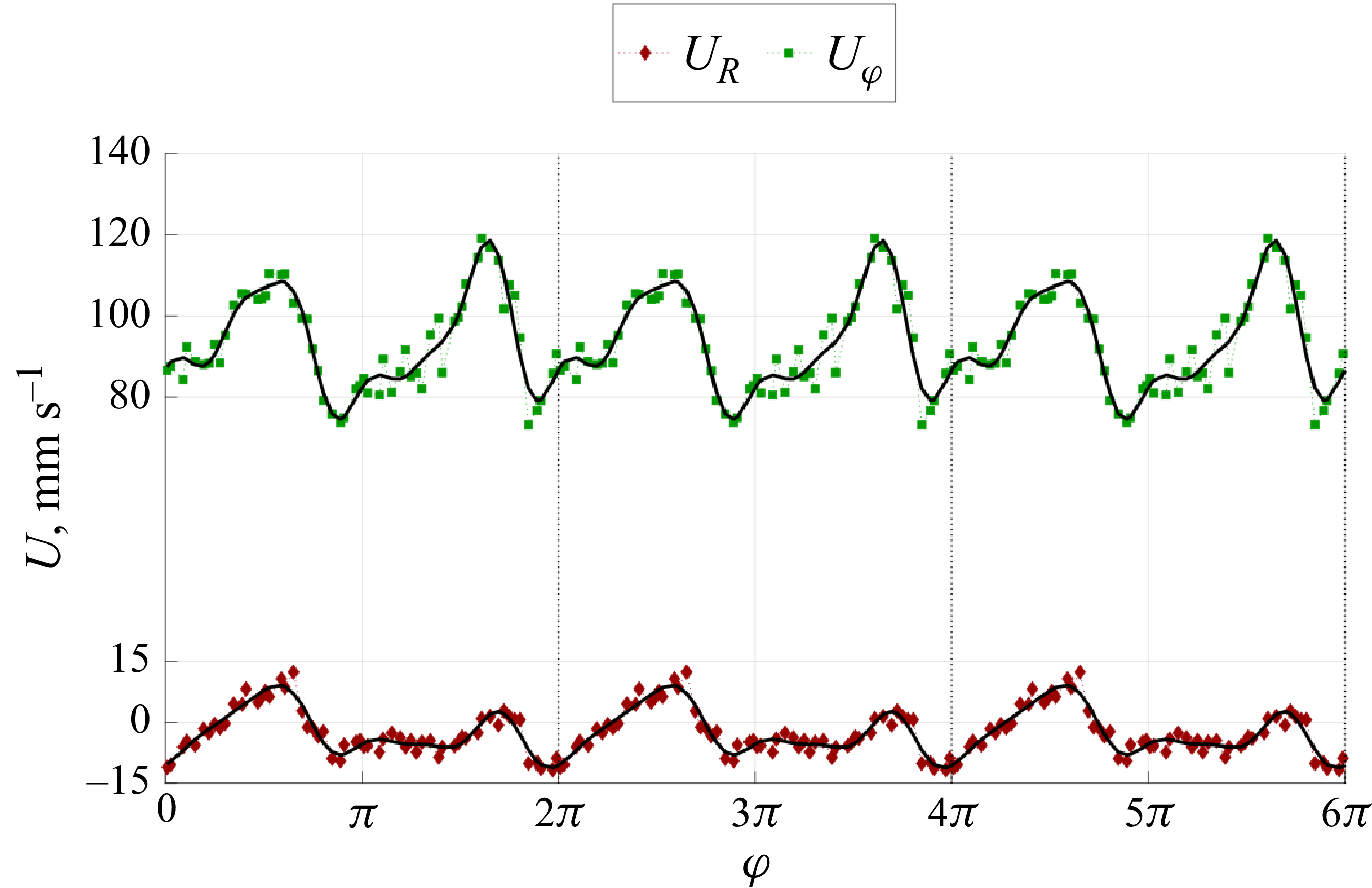
The spatial section of the velocity signal at a fixed point of time (figure 9) shows the periodicity of the change of both components $V_{\varphi }$ and $V_{r}$ along the angular coordinate $\varphi$ . Fourier analysis shows that the dominant mode in angle is $m=2$ , although the signal of the azimuthal velocity component also contains multiple higher harmonics.

Figure 9.

The spatial section of the velocity signals at fixed point of time along the azimuthal coordinate. The approximation of experimental data by a linear combination of harmonics is marked with a solid black line.

The distribution of the velocity components along the radial coordinate (figure 10) depends on the wave phase. At the moment between the periods of passage of the wave crests through the observation point $\varphi = \textit{const}$ , the azimuthal velocity profile is linear (figure 10 a), which indicates a quasi-solid-body rotation of the liquid. At the moments of time corresponding to the passage of the wave through the azimuthal section under consideration, the velocity profile $V_{\varphi }$ is distorted. In the region $r\in (0, 0.7R)$ , the velocity profile is close to linear, and at $r\in (0.7R, 1.0R)$ the angular velocity remains constant along the radial coordinate.

Figure 10.

Distribution of velocity components along the radial coordinate at the point $\varphi =\pi$ : $V_{\varphi }$ (a), $V_{r}$ (b). The numbers in the legend mark profiles at different moments in time: 1. the passage of the wave maximum through the point in question, 2. the passage of the wave minimum through the point in question, 3. the average profile between 1 and 2.

At the same time, the radial flow at the moments of time between the periods of passage of the wave crests is convergent (figure 10 b). The velocity $V_{r}\lt 0$ in the entire region. The highest intensity of the radial flow is achieved precisely in the region of wave motion $r\in (0.6R, 0.8R)$ . When the wave passes through the selected section $\varphi = \textit{const}$ , the flow direction locally changes and an intense divergent flow is observed in a narrow band along the angular coordinate (figure 8). Analysis of the phase change (figure 6) shows that the radial flow associated with the wave motion on the metal surface is slightly ahead of the radial flow by phase.

Figure 11(a) represents a spatio-temporal map of the vertical velocity component obtained by the ultrasonic sensor. The flow in the central part of the cell is downward across its entire height. Despite the oscillatory nature of the motion in the near-surface layer, the vertical velocity component shows a slight change over time. Figure 11(b) represents the time-averaged velocity profile (the grey area marks the amplitude of velocity oscillations). The highest downward flow velocity is observed in the transition region of the cell with a diameter of $d_{1}=200$ mm into a cell with a diameter of $d_{2}=100$ mm. At the same time, in the region of $z\in (106, 110)$ mm, a sharp jump in velocity occurs, apparently associated with instability processes between two counter-rotating volumes of fluid.

Figure 11.

Spatio-temporal map of the $z$ -component of velocity (a), time-averaged profile (b) and velocity time series (c) in two space sections marked by lines on the velocity map.

The time series of the velocity in two space sections ( $z=55$ and $z=150$ mm marked with a dotted lines on the velocity map) is presented in figure 11(c). The choice of sections is due to the different natures of the flow in the selected areas. The velocity pulsations are irregular. The flow in the lower part of the cell has pronounced periodic pulsations with a frequency of $0.2$ Hz. Wavelet analysis of the flow in the central part of the cell shows that there are no distinguished frequencies in the velocity signal of this area.

Summarising the obtained experimental data on the flow, it is possible to describe the generated flow as a quasi-solid-body rotation of the liquid metal in the upper part of the cell that generates a toroidal vortex with a pronounced downward flow in the centre of the volume. At the same time a pair of surface waves arises, moving co-directionally with the main azimuthal flow, but ahead of it. In the lower part of the cell, a convergent flow is formed in the form of a toroidal vortex with a downward flow, also directed downwards, but rotating azimuthally in the opposite direction (in accordance with the specified direction of the RMF in the lower inductor).

3.4. Multiwave mode

With further increase of the $\textit{Ta}_{2}$ parameter an irregular flow of complex topology is realised. This mode occupies an intermediate position in the region of parameters $\textit{Ta}_{1}, \textit{Ta}_{2}$ . At $\textit{Ta}_{1} \gg \textit{Ta}_{2}$ , quasi-solid-body rotation of positive direction (in the selected coordinate system) is realised. At $\textit{Ta}_{1} \ll \textit{Ta}_{2}$ , rotation with negative direction is realised. And at $\textit{Ta}_{1} \sim 50 {\times}\textit{Ta}_{2}$ surface waves arise. In intermediate regions ( $10\lt \textit{Ta}_{1} /\textit{Ta}_{2}\lt 20$ ) of the force parameters, the balance of forces does not allow stable wave motion to develop, and at the same time, none of the force components $f_{1}, f_{2}$ is strong enough to create uniform rotation. Thus, there is a mode in which the metal surface is not involved in large-scale motion, but small-scale hydrodynamic structures arise chaotically on the surface. Weak waves arise and fade, vortices with a lifetime of several seconds are formed. Some of these vortices manage to merge into one. An important feature of this mode is that the metal surface remains unperturbed (there is no significant rise in the fluid level and no formation of a large-scale funnel) even at large values of $\textit{Ta}_{1}$ and $\textit{Ta}_{2}$ .

Figure 12 represents examples of the instantaneous flow velocity field in Cartesian and radial coordinates. The non-periodic velocity pulsations exist in both the radial and azimuthal directions on the background of a relatively weak large-scale azimuthal flow. This mode can be generally described as ‘seething’ of the fluid. We will conditionally call this regime multimode or multiwave flow, indicative of the multi-scale nature of the vortices arising on the metal surface. The rotation direction of the average large-scale flow is determined by the dominant component of the force $f_{1}$ near the free surface.

Figure 12.

Instantaneous velocity field on the free surface of liquid metal in multiwave mode: (a) full field in the Cartesian coordinate system, (b) radial component field in a cylindrical coordinate system, (c) azimuthal component field in a cylindrical coordinate system. Here, $\textit{Ta}_{1}=2.3 {\times}10^{10}$ , $\textit{Ta}_{2}=1.6 {\times}10^{9}$ .

Figure 13.

Instantaneous velocity field on the free surface of liquid metal in tornado-like vortex mode: full field in the Cartesian coordinate system (a), radial component field in a cylindrical coordinate system (b), azimuthal component field in a cylindrical coordinate system (c). Black arrow represents direction of fluid rotation. Here, $\textit{Ta}_{1}=1.6 {\times}10^{10}$ , $\textit{Ta}_{2}=3.3 {\times}10^{9}$ .

Near the boundary of the multimode mode existence region, there is a area of $\textit{Ta}_{1}$ that is large enough to generate intense swirling of the fluid with the formation of a funnel, but which does not exceed $\textit{Ta}_{2}$ sufficiently to ensure uniform rotation of the metal in the near-surface layer. In this region, the liquid metal flow is a superposition of uniform rotation of the upper layer in the positive direction and multimode small-scale vortices on the partially disturbed surface of the funnel.

3.5. Tornado-like mode

A further increase in $\textit{Ta}_{2}$ leads to the fading of the liquid ‘seething’ and the formation of a tornado-like vortex near the central axis of the cell. This mode is observed at $5\lt \textit{Ta}_{1} /\textit{Ta}_{2}\lt 10$ , but the condition $\textit{Ta}_{2}\gt \textit{Ta}_{1}$ is still not satisfied (i.e. before the formation of quasi-solid-body rotation of negative direction).

Figure 13 shows the representative velocity fields on the surface of the liquid metal during the emergence of a tornado-like flow. The fluid is rotating relatively slowly in the positive direction with the formation of a funnel in the central part of the cell (the brightly coloured region near the centre in figure 13 a). The vortex funnel has a diameter of approximately 10 % of the cell diameter $d_{2}$ for the regime with moderate Taylor numbers and grows with their increase. The vortex itself is characterised by an intense and highly localised convergent liquid flow also with a positive spin. The flow velocity near the forming funnel increases sharply. This mode is clearly demonstrated in figure 14. The depression formed on the surface is typical for a tornado in liquid metals (Vogt et al. Reference Vogt, Grants, Eckert and Gergeth2013), which is why we call this flow mode tornado-like. It should also be noted that the local velocity pulsations observed in figure 13 near the cell boundaries are associated with oscillations of the liquid surface due to the formation of waves (which is clearly visible in the storyboard figure 14).

Figure 14.

Storyboard of the liquid metal surface in the tornado-like vortex mode, taken with a time step of 0.35 s (from left to right, from top to bottom). The yellow arrow shows the direction of the vortex axis precession.

Apparently, the force action from the upper inductor is not limited to creating motion in the near-wall region. Precession of the vortex relative to the cell axis is observed, as shown in figure 14. The linear frequency of precession is approximately 0.36 Hz and increases with increasing absolute values of the Taylor numbers in the region of their constant ratio. The centre of the vortex describes a circle with a radius approximately equal to the funnel diameter. The direction of precession coincides with the direction of the electromagnetic force $f_{2}$ acting from the lower inductor (positive rotation).

Based on the known precession period and the position of the vortex centre, it is possible to estimate the linear velocity of the tornado-like funnel along the circumference as $V_{\textit{prec}}\approx 20$ mm s⁻¹. At the same time, optical measurements show that the velocity of the liquid in the area of the funnel reaches 70 mm s⁻¹.

To the authors’ knowledge, such a regime has not been previously observed in experimental works with liquid metals. The key features of the tornado-like flow obtained by us are the stability of the vortex and the precession of the rotation axis. The vortex structure is preserved for a long time (hundreds of vortex revolutions). According to Vogt et al. (Reference Vogt, Grants, Eckert and Gergeth2013), this may indicate that conditions with a low level of turbulence with a developed large-scale flow (the Reynolds number of the large-scale flow is $\textit{Re}\sim 2.3 {\times}10^4$ ) were created in this configuration. Starting from the moment of the emergence of a convergent swirling flow in the near-surface layer, the vortex axis rarely coincides with the axis of the cylindrical cell, which distinguishes the observed mode from the flows described in similar works (Vogt et al. Reference Vogt, Grants, Eckert and Gergeth2013; Grants et al. Reference Grants, Zhang, Eckert and Gerbeth2009; Kharicha et al. Reference Kharicha, Al-Nasser, Barati, Karimi-Sibaki, Vakhrushev, Abdi, Ludwig and Wu2022).

The authors offer the following explanation for the phenomenon of vortex axis precession. According to the works of Ward (Reference Ward1972) and Church et al. (Reference Church, Snow and Agee1977), in which tornadoes of various types were successfully modelled in laboratory conditions in air, a necessary condition for the emergence of such vortex structures is the presence of two zones. A converging layer, in which a rotating converging flow is created by a special fan and rotating net, and a convection zone above it with an ascending flow, in which tornadoes arise. The liquid, moving through the converging layer, acquires the necessary swirl and enters the convection zone at a certain angle of inflow. The flow mode realised largely depends on this angle. Another important parameter, called the configuration ratio, is the ratio of the convection zone diameter to the height of the converging layer. In real tornadoes, its value can be approximately 5. According to Ward (Reference Ward1972), for more than one vortex to exist, its value must be greater than one. In our laboratory set-up, probably, the lower narrow cylinder (or its upper part) acts as a converging layer, and the upper wide one acts as a convection zone. In this case, the configuration ratio is at least 1.4. The ratio of magnetic Taylor numbers $\textit{Ta}_{1}$ and $\textit{Ta}_{2}$ could act as some analogue of the angle of inflow parameter.

The main difference between our configuration and the mentioned laboratory models (Ward Reference Ward1972; Church et al. Reference Church, Snow and Agee1977) is the absence of a transit flow through the cell. Using the UDV probe, we measured the vertical velocity component on the cell axis (figure 15). The rotational motion of the fluid generated by electromagnetic forces creates a predominantly downward flow on the central axis. Due to the finite volume of the fluid, a predominantly lower-intensity upward flow occurs in the rest of the cell. Since a tornado-like vortex can only occur in a zone with a volumetric upward flow, in our set-up the vortex occurs at some distance from the central axis of the cell and precesses under the action of electromagnetic forces.

Figure 15.

Spatio-temporal map of the $z$ -component of velocity (a), time-averaged profile (b) and velocity time series (c) in two space sections marked by lines on the velocity map.

The downward flow velocity in the cell centre turns out to be comparable to the velocity of the rotational motion of the liquid carried away by the precessing vortex. The oscillatory nature of the large-scale motion is also manifested in the vertical flow. The spatio-temporal velocity map shown in figure 15(a) displays the periodic change in the flow velocity along the entire cell axis. Figure 15(c) shows the time scan of the signal at point $z=150$ mm. It is evident that the flow is indeed downward most of the time, and its velocity varies within wide limits from $25$ to $100$ mm s⁻¹. However, sometimes the flow becomes upward, irregularly and for a very short time with velocities up to $50$ mm s⁻¹. The authors associate such events with the entry of a tornado tube, inside which the flow is known to be upward, into the field of view of the UDV beam. At such moments of time, the vortex funnel on the surface also leaves the trajectory shown in the figure 14 and ends up on the cell axis or in close proximity to it. Fourier analysis of this signal shows that the oscillation frequency of the vertical velocity component is approximately $0.2$ Hz, i.e. it turns out to be significantly less than the precession frequency of the funnel on the liquid surface.

Although the tornado-like vortex exists in the entire range of $5\lt \textit{Ta}_{1} /\textit{Ta}_{2}\lt 10$ , the behaviour of the vortex changes somewhat depending on the proximity to the range boundaries. At $ \textit{Ta}_{1} /\textit{Ta}_{2}\sim 5$ the tornado-like vortex exhibits stable precession around the cell axis. At $ \textit{Ta}_{1} /\textit{Ta}_{2}\sim 10$ the motion of the vortex centre along the azimuthal coordinate turns out to be chaotic. The vortex appears at the same distance from the cell axis as during precession, exists motionless for several seconds and then randomly changes its angular position without changing the radial coordinate. The mode turns out to be stable, in the sense that the `jumps’ are repeated throughout the entire experiment at unequal intervals. Let us conditionally call such a flow a `jumping tornado’ to separate the emerging hydrodynamic regimes.

3.6. Regime map

The aforementioned regimes (modes) are realised depending on the Taylor number, $\textit{Ta}_{1}$ and $\textit{Ta}_{2}$ , ratio, therefore, it is possible to construct a regime map on the plane of governing force parameters. Numerical modelling of flows in a full three-dimensional formulation is significantly more computationally intensive compared with experimental observation of hydrodynamic structures. Therefore, the map of hydrodynamic regimes (figure 16) realised in a T-shaped cell was produced based on 100 experimental data points. Within the considered parameter range, nine distinct regimes can be identified, differing in the structure of the resulting surface flows.

Figure 16.

Flow regime map observed in the T-shaped cell as a function of electromagnetic forcing parameters in the upper ( $\textit{Ta}_{1}$ ) and lower ( $\textit{Ta}_{2}$ ) cell sections. Coloured symbols show stable modes and open symbols marks transitional regime between two adjacent modes.

At low values of $\textit{Ta}_{1}$ and $\textit{Ta}_{2}$ , the fluid flows generated within the volume are insufficiently intense to induce motion in the near-surface layers of the metal. Consequently, in the vicinity of zero, there exists a small parameter region where the free surface of the metal remains in a state of mechanical rest.

The quasi-solid-body rotation regime of the upper layer is realised within a narrow band where $\textit{Ta}_{1}\gg \textit{Ta}_{2}$ . An increase in $\textit{Ta}_{2}$ at $\textit{Ta}_{1}\neq 0$ leads to a fundamental restructuring of the flow pattern and the formation of three surface waves at the metal–air interface. This regime is characterised by a flattening of the metal surface compared with the funnel shape observed under quasi-solid-body rotation, and exhibits similarity to the double hydrodynamic structure described in § 3.3. Three wave crests, symmetrically positioned relative to the cell centre, propagate along circular trajectories co-directional with the large-scale fluid rotation. The triple-wave pattern persists only within an extremely narrow parameter range and transitions to a double-wave regime upon further increase of $\textit{Ta}_{2}$ , achieved through wave pair merging and enlargement of the third wave, thereby restoring axial flow symmetry. Thus the area of existence of the double-wave regime is much wider than that of the triple-wave regime.

Further increase in $\textit{Ta}_{2}$ leads to the breakdown of the double-wave flow pattern and the emergence of a multiwave regime. In the parameter region where $\textit{Ta}_{1}\gtrsim 4 {\times}10^{10}$ , a hybrid regime is observed that combines features of quasi-solid-body rotation with multiscale vortex structures. The multiwave regime persists within a broad parameter cone defined by $\textit{Ta}_{1}\sim 10 {\times}\textit{Ta}_{2}$ , occupying an intermediate position on the regime map that separates domains of predominant fluid rotation in positive and negative directions (dominated by $f_{1}$ or $f_{2}$ forces, respectively).

Above the diagonal of the regime map lies the domain of tornado-like flows, which can be conditionally divided into two sub-regions: precessing tornado and jumping tornado. At high $\textit{Ta}_{1}$ values, the developing tornado-like vortex exhibits chaotic displacement along the angular coordinate while maintaining its axial position for several seconds before each new ‘jump’. At lower $\textit{Ta}_{1}$ values, the tornado axis undergoes continuous precession about the axis of the T-shaped cell. In both cases, the radial position of the vortex remains constant, with tornado axis motion restricted to angular displacement.

In the region of relatively small $\textit{Ta}_{1}$ values, the force impact from the lower inductor becomes dominant, generating intense rotation at the liquid metal surface that leads to deep narrow (but sufficiently wider than in the tornado-like regime) funnel formation. The fluid rotates in the negative direction within the chosen coordinate system, consistent with the direction of the electromotive force produced by the lower inductor.

4.1. Top layer rotation

The top layer rotation mode occurs when the electromagnetic force ( $f_{1}$ in figure 18) acts solely on the upper part of the cell ( $\textit{Ta}_{2}=0$ ). The intense azimuthal rotation of the fluid ( $V_{1}$ in figures 18 and 19) induces secondary poloidal flows due to Ekman pumping ( $V_{3}$ in figure 18) (Davidson, Short & Kinnear Reference Davidson, Short and Kinnear1995).

Figure 18.

Sketch of the main flows forming in the cell: $V_{1}$ – intense azimuthal rotation of the fluid in the top layer, $V_{2}$ – intense azimuthal rotation of the fluid in the bottom layer, $V_{3}$ – secondary poloidal flows due to Ekman pumping in the top layer, $V_{4}$ – secondary poloidal flows due to Ekman pumping in the bottom layer, $V_{5}$ – Taylor–Görtler vortices in the top layer, $V_{6}$ – Taylor–Görtler vortices in the bottom layer, $V_{7}$ – unsteady medium-scale vortices, $V_{8}$ – tornado-like large-scale vortex. Vertical and two horizontal sections are represented.

Figure 19.

Instantaneous isosurfaces’ velocity field in top layer rotation mode: azimuthal (a) and vertical (b) components. Here, $\textit{Ta}_{1}=9.8 {\times}10^{9}$ , $\textit{Ta}_{2}=0$ .

The physical mechanism of pumping is attributed to the formation of differential rotation near the end walls of the cylindrical cell, generating an axial gradient of centrifugal force and, consequently, pressure. The liquid metal moves from the cell axis toward the vertical wall in the region affected by electromagnetic forces. Near the vertical wall, the fluid reverses direction and returns to the cell axis along regions adjacent to the horizontal walls. The spatial structure of the poloidal flow takes the form of two tori.

Near the solid concave walls (guiding surfaces of the cylindrical cell), Taylor–Görtler vortices ( $V_{5}$ in figure 18) (Saric Reference Saric1994) emerge in the shape of longitudinal vortex rolls aligned with the flow. These vortices contribute to the formation of the poloidal velocity component, but their scale is comparable to the boundary layer thickness. Taylor–Görtler vortices arise in a fluid rotating in an RMF as a result of instability driven by the gradient of centrifugal force normal to the solid concave wall (Richardson Reference Richardson1974; Kaiser & Benz Reference Kaiser and Benz1998). The vortices in the shape of a longitudinal vortex aligned with the flow arise when the Taylor number exceeds a critical value $Ta^{cr}\sim 10^{5}$ (Grants & Gerbeth Reference Grants and Gerbeth2002; Stiller, Fraňa & Cramer Reference Stiller, Fraňa and Cramer2006). Further increase of $Ta$ decreases the vortex lifetime (Vogt et al. Reference Vogt, Grants, Räbiger, Eckert and Gerbeth2012). As a result, at sufficiently large supercriticality, the flow becomes turbulent and identification of Taylor–Görtler vortices becomes difficult against the background of multiple irregular velocity pulsations (Stiller et al. Reference Stiller, Fraňa and Cramer2006; Vogt et al. Reference Vogt, Grants, Räbiger, Eckert and Gerbeth2012). In practice, the critical values $Ta^{cr}\sim 10^{5}$ for liquid metals in an external RMF of industrial frequency ( $\sim 50$ Hz) are such that the magnetic field induction has an amplitude ( $B\sim 1$ mT) (Kaiser & Benz Reference Kaiser and Benz1998). This threshold is easily overcome in many technological devices. The formation of these vortices in our formulation is influenced not only by the azimuthal flow, but also by the emerging large-scale secondary poloidal flow described above. The scale of Taylor–Görtler is comparable to the boundary layer thickness.

Initially, axisymmetric oscillations of large-scale poloidal Ekman vortices are supplemented by the development of Taylor–Görtler vortices. This leads to oscillations of the resulting large-scale poloidal flow in the azimuthal direction. In this case, the oscillations of the vertical velocity component become desynchronised in time, which is illustrated by figure 21(b). This may indicate the formation of a spiral flow.

Observations of flow evolution reveal that these vortices are not stationary but sporadically form and migrate toward the upper or lower wall, acquiring a helical spatial structure. Additionally, it should be noted that, in this mode, the primary large-scale azimuthal vortex and secondary azimuthal vortices exhibit only weak penetration into the lower-layer region.

4.2. Bottom layer rotation

Bottom layer rotation mode occurs when the electromagnetic force ( $f_{2}$ in figure 18) acts exclusively on the lower part of the cell ( $\textit{Ta}_{1}=0$ ). In this mode, the lower cell section develops an azimuthal flow in the cylinder’s central region ( $V_2$ in figure 18), accompanied by a secondary poloidal flow forming two toroidal structures ( $V_4$ in figure 18) induced by Ekman pumping. The flow actively propagates into the upper cell section (figure 20), eventually occupying the entire fluid volume.

Figure 20.

Instantaneous isosurfaces’ velocity field in bottom layer rotation mode: azimuthal (a) and vertical (b) components. Here, $\textit{Ta}_{1}=0$ , $\textit{Ta}_{2}=3.6 {\times}10^{9}$ .

In the lower cell section, rotation generates small-scale spiral wall vortices ( $V_6$ in figure 18) due to Taylor–Görtler instability (figure 21). The upper section develops differential rotation of the liquid metal, with faster rotation near the cylinder axis compared with peripheral regions. This process triggers Kelvin–Helmholtz instability in the upper half-cell (Drazin & Reid Reference Drazin and Reid1981).

Figure 21.

Spatio-temporal maps of the $V_x$ velocity component for profiles located along the diameter near the upper boundary $z=245$ mm (a); $V_z$ component near the lateral boundary of the cell $x=95$ mm, $y=0$ (b).

Visually, this flow instability manifests as several unsteady medium-scale vortices ( $V_7$ in figure 18) advected by the primary large-scale flow in the central region. Subsequently, the flow engages the wall-adjacent fluid in the upper cell section, leading to Taylor–Görtler instability ( $V_5$ in figure 18) on the upper sidewall. Meanwhile, vortices generated by both Kelvin–Helmholtz and Taylor–Görtler instabilities become less pronounced. The large-scale vortex becomes more azimuthally homogeneous, with its rotational axis (where azimuthal velocity vanishes) aligning with the cell axis.

4.3. Tornado-like mode

When an electromagnetic force acts simultaneously in both the top and bottom parts of the cell, the fluid is gets involved in azimuthal motion in opposite directions along the height of the cylindrical volume. Not only do the aforementioned secondary flows and instabilities develop in the upper and lower sections of the cell but additional effects also arise under such forcing conditions.

With more intense forcing in the bottom part of the cell, the peripheral region of the top layer rotates in the opposite direction relative to the lower layer (figure 22). This enhances differential rotation in the upper layer and, consequently, intensifies secondary vortices due to the Kelvin–Helmholtz instability. As a result, within a sufficiently narrow range of the parameters $\textit{Ta}_1$ and $\textit{Ta}_2$ a tornado-like structure emerges. The rotation axis of the large-scale vortex in the top part of the cell moves along a circular trajectory around the cell axis ( $V_{8}$ in figure 18).

Figure 22.

Instantaneous isosurfaces’ velocity field in tornado-like mode: azimuthal (a) and vertical (b) components. Here, $\textit{Ta}_{1}=1.6 {\times}10^{10}$ , $\textit{Ta}_{2}=3.3 {\times}10^{9}$ .

Figure 23.

Spatio-temporal diagrams of the $V_y$ velocity component for profiles located along the diameter near the upper boundary $z=245$ mm (a); the axis of the cell $x=y=0$ (b).

The vortex precession is clearly visible in the spatio-temporal map (figure 23). The abscissa axis represents time, while the ordinate axis corresponds to the coordinate along the diameter, with colour gradations indicating the magnitude of the azimuthal velocity at a given point. Oscillations in the region with near-zero velocity exhibit a harmonic dependence characteristic of circular motion. The oscillation frequency is approximately equal to the inverse of the large-scale vortex rotation period. The inclined dark bands characterise the motion of the spiral-shaped large-scale vortex. In the near-wall region, Taylor–Görtler vortices are observed.

4.4. Double-wave mode

The most interesting regime in terms of the spatial flow structure is the double-wave mode, which arises in simulations when the electromagnetic forcing intensity slightly dominates in the top part of the cell. In this case, all previously described instability effects remain valid, but an additional phenomenon emerges.

An analysis of the evolution of spatial components of the velocity and pressure fields reveals that, for the given parameter ratios, the competition between secondary structures driven by Ekman pumping in the top and bottom parts of the cell begins and plays a key role against the background of the primary flows (figure 24). When either the lower or upper layer rotates alone, this structure spreads throughout the entire cell and persists in a steady state without significant oscillations. However, when the fluid layers rotate in opposite directions, neither of the secondary structures becomes dominant in this regime. Instead, they alternately replace each other, as illustrated by the spatio-temporal diagram of the vertical velocity component (figure 25 a).

Figure 24.

Instantaneous isosurfaces’ velocity field in double-wave mode: azimuthal (a) and vertical (b) components. Here, $\textit{Ta}_{1}=2.3 {\times}10^{10}$ , $\textit{Ta}_{2}=4.8 {\times}10^{8}$ .

Figure 25.

Component $V_z$ of the three-dimensional velocity field: space–time diagram in a vertical section near the wall of the narrow part of the T-shaped cell $x=45$ mm, $y=0$ (a); the field of the velocity modulus on the horizontal region located near the upper surface of the cell $z=245$ mm (b).

The structures generated by Ekman pumping lose their axisymmetric toroidal shape and assume the form of two deformed rings rotating around the cell axis. This results in the formation of a boundary between a pair of hydrodynamic structures where the planar velocity components, as well as the pressure, are close to zero. In the near-surface layer, the boundary line takes the shape of a two-bladed propeller (figure 25 b) rotating around the cell axis. The hydrodynamic structures originate deep within the cell, so the two-wave or two-jet flow regime can emerge with either a rigid or free upper boundary.